Computer Modeling in Engineering & Sciences

DOI: 10.32604/cmes.2022.020331

ARTICLE

B-PesNet: Smoothly Propagating Semantics for Robust and Reliable Multi-Scale Object Detection for Secure Systems

Yunbo Rao1,2,*, Hongyu Mu1, Zeyu Yang1, Weibin Zheng1, Faxin Wang1, Jiansu Pu1 and Shaoning Zeng2

1School of Information and Software Engineering, University of Electronic Science and Technology of China, Chengdu, 610054, China
2Yangtze Delta Region Institute (Huzhou), University of Electronic Science and Technology of China, Huzhou, 313000, China
*Corresponding Author: Yunbo Rao. Email: raoyb@uestc.edu.cn
Received: 17 November 2021; Accepted: 26 January 2022

1  Introduction

In recent years, computer vision has thrived with the support of deep learning [1 –7]. Object detection manifests great practical and research value in many subfields of computer vision. Many object detection approaches proposed in earlier years [8,9] were built based on designing features manually. The shortcoming of those detectors is a lack of generalization. Now, more and more state-of-the-art detection models using convolution neural networks (CNNs) [10,11] were presented. By combining with CNN, object detectors display great power by addressing complex tasks. There are two kinds of detectors: (1) two-stage method [12–20] and (2) one-stage method [21–30]. As for the two-stage detector, firstly, the detector tries to find a set of candidate boxes containing objects. These boxes will introduce important semantic information to classification and regression in the second part. Two-stage methods obtained a better accuracy on PASCAL VOC [31] and MSCOCO [32] than one-stage detectors. Object classification and bounding box regression will take place simultaneously in one-stage approaches. These are very important in building a secure system using image detection.

A new framework termed region proposal network (RPN) was proposed by Ren et al. [15] in 2017. They made a detector titled Faster R-CNN, which used RPN to find the bounding box. Object detection was regarded as a regression other than classification task in which you look only once (YOLO) by Redmon et al. [22], which splits the input image into multiple parts for predicting the object. Liu et al. [21] merged features from different layers to make an object prediction in a detector, called single shot detector (SSD). SSD has a better performance in comparison with YOLO. Pang et al. [25] exposed some imbalances during the phase of detection: sample imbalance and feature imbalance. Consequently, the IoU-balanced, feature pyramid and a new loss function termed L1 loss is proposed to moderate those imbalances in Libra R-CNN. Despite its attempts to improve themselves, two-stage detectors were still better than one-stage detectors till the advent of RetinaNet. Lin et al. [24] depicted that the severe imbalance between the foreground and background samples is the critical determinant to influencing the accuracy of one-stage detectors, and a newly-designed loss function termed focal loss was proposed to relieve such imbalance.

However, the one-stage approaches and two-stage approaches mentioned above have some weaknesses. The main limitation of the popular methods is the insensitivity to multi-scale objects. First, in most detection datasets, the scales of objects vary a wide range. What is worse, there are some extremely big or small objects. Such scale variation will make it difficult for detectors to take into account the different scales, hence weakening the accuracy of those detectors. All of the methods summarized above have to reshape the input image to a small size at the beginning of training, which inevitably misses some semantic information. Furthermore, more information will be lost in the following convolution process. Accordingly, traditional detectors have lousy performance for this multi-scale object detection. Second, there is a class imbalance problem in existing datasets. The amount of easily classified samples is much more than those hard to classify. Consequently, the detector is not robust enough.

Based on the above shortcoming of those networks, a new network entitled balanced Pre-ReLU ResNet (B-PesNet) is proposed in our work. As a significant idea, we propose a Pre-ReLU residual block that aims to prevent the degeneration of the deep networks, and then we could build a deeper network without losing semantic information and a new loss function for addressing the extremely class imbalance. The main contributions of our work are from two aspects:

    (i)  A new residual block within a Pre-ReLU is proposed, which is proven to mitigate the degradation problem of deep neural networks when the network becomes deeper. The reason for the degradation of deep neural networks is that too much semantic information is lost in the repeated convolution process. However, our Pre-ReLU retains shallow semantic information so that the deep neural unit can also use shallow information to calculate, thus solving the degradation problem. This brings a more reliable model for many secure systems.

  (ii)  Balanced Loss (BL) is suggested for solving class imbalance and helping produce a model more reliable than YOLOv2 [27], YOLOv3 [28], and YOLOv4 [26]. Compared with YOLOv5 [33], we found that the accuracy of B-PesNet is comparable, and the speed is slightly inferior. By introducing weight factor α, BL balances the proportions of different samples in the gradient and prevents negative samples from dominating the direction of gradient descent, thereby solving the problem of class imbalance. We give a mathematical deduction, as well as extensive experimental evaluations, to confirm its crucial role for a reliable solution.

The following content in this paper is summarized as follows. We concisely retrospect the research concerned with our work in Section 2. Then, particulars of our approach are given in Section 3, where we introduce our B-PesNet. In Section 4, we will state our datasets and evaluation metrics. Experimental results are listed in Section 5. Finally, Section 6 sums up our outcomes and offers some standpoints for future work.

2  Related Work

With the widespread utilization of deep learning, object detection approaches have evolved from traditional algorithms based on manual design to automatic extraction of features based on deep learning. Modern object detectors can be approximately divided into one-stage [21–24,26–30] and two-stage algorithms [12 –20].

2.1 One-Stage Methods

The one-stage method combines extraction and detection into a whole. One-stage approaches will not explicitly extract candidate regions but directly obtain the final detection result. Liu et al. [21] proposed Single Shot Multi-Box Detector (SSD), which utilizes fused features from different layers of the network. Redmon et al. [22] proposed You Only Look Once (YOLO). YOLO integrates the information of the entire image to predict the object at each position. It regards the entire image as input and predicts in the original image: the category and positioning-related information of each part in the area. Lin et al. [23] proposed feature pyramid networks (FPN). The main problem of this method is the insufficiency of object detection in dealing with multi-scale changes. This network architecture can increase the feature map with various semantic information, but rich spatial information is integrated under the premise of less calculation.

2.2 Two-Stage Methods

The working method of the two-stage detection method is to first generate a set of region proposals and then classify and regress these proposals. Compared with the one-stage method, the two-stage method is more accurate but less efficient. Firstly, 2000 region proposals were selected through selective search, and each region proposal will be input into CNN to extract features. And then, the classifier will utilize these features to classify. Subsequently, Girshick et al. [12] proposed an improved version of R-CNN, which is termed Fast R-CNN. For R-CNN, the disadvantage is that the efficiency begins to decline during preprocessing. For instance, use selective search to track potential bounding boxes as input. This search method will make the model spend much time on useless data. Fast R-CNN introduces a new layer of the network, named ROI Pooling, which cleverly puts regression into the network and fuses it with classification into a multi-task model. Ren et al. [15] proposed Faster R-CNN. On the basis of Fast R-CNN, they added a newly-designed structure termed region proposal network (RPN). Therefore, the model will utilize RPN to find candidate boxes, which further improves efficiency.

3  Our Method

In this section, we firstly introduce the B-PesNet. Then BL is proposed to balance the class imbalance during the network training.

3.1 Pre-ReLU

ResNet [34] solved the degradation problem of deep neural networks. However, after deepening the network without limitation, the network degradation problem still exists. It is considering that the residual structure tackles the problem of network degradation by the skip connection, which retains the shallow information. After a large number of experiments and rigorous mathematical verification, it has been found that if we put the ReLU [35] layer in front of the convolution layer, we can get a Pre-ReLU residual block, and improve its performance.

We introduce the Pre-ReLU residual block starting from the standard residual unit:

yl=h(xl)+F(xl,Wl). (1)

xl+1=f(yl). (2)

where xl is the input of the l th residual unit, and Wl means a set of weight factors associated with the l th residual unit. f denotes the ReLU, h means a skip connection: h(xl)=xl, and F represents the residual function. As it is known to all, the advantage of ResNet is contributed by the skip connection. This design is able to propagate more lower layers information to the deeper layers. However, in real training, we found that deeper ResNet caused a worse degeneration.

Then, if f is a skip connection: xl+1 = yl, we can convert Eq. (2) into Eq. (1):

xl+1=xl+F(xl,Wl). (3)

For the whole network, it becomes:

xL=xl+∑i=lL−1F(xi,Wi), (4)

where xL means the input of any residual unit that is behind the l th unit. Then, we found that, for any unit, the information is able to be propagated from one unit to the others.

In order to build a gate, which is able to propagate information without loss from shallow to deep layer, we put a ReLU layer in front of the convolution layer. As we assumed, the Pre-ReLU residual block builds a clean pathway from shallower to a deeper layer. Then more features can be reserved during convoluting.

3.2 Feature Map Division

To decrease the number of parameters and enhance the running speed, we split the feature map into many groups.

First, we divide the feature map into an equal dimension at the dimension level and divide it into multiple groups with the same dimension. The workflow is shown in Fig. 1.

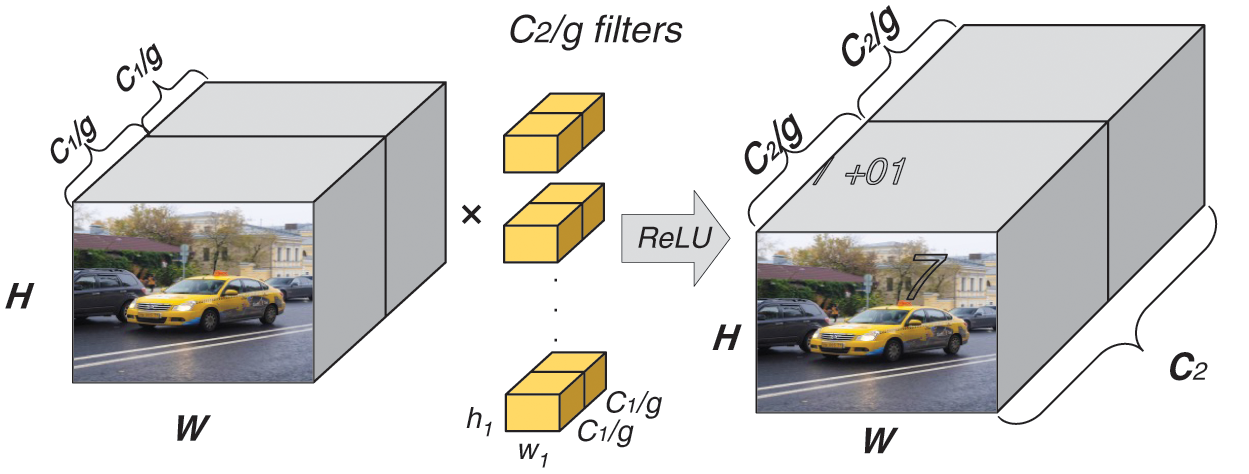
Figure 1: The workflow of dividing. H represents the height of the feature map, and W means the width of the feature map. c1g expresses the dimension of each group feature map

Assume the size of the input image is H×W×c1, and divide it into g groups, then every group has the same size as H×W×c1g, the corresponding convolution kernel size is h1×w1×c1g, and there are c2g kernels. Then perform the SAME convolution, the size of each output is H×W×c2g. Afterwards, concatenate the results of g groups, we will obtain an output feature map whose size is H×W×c2 finally. The amount of parameters of this convolution layer is:

h1×w1×c1g×c2g×g=h1×w1×c1×c2×1g. (5)

3.3 B-PesNet

Pre-ReLU residual block contains three convolutional layers. The architecture of the block is shown in Fig. 2, and the convolution kernel sizes are 1×1, 3×3, and 1×1, respectively. According to the characteristics of the Pre-ReLU block, we construct a feature extractor named Pre-ReNet, which contains 50 convolutional layers. The net can be divided into five parts based on the size of the output image. The first part is a 7×7 convolution kernel, the second part contains three residual blocks, the third part contains four residual blocks, the fourth part contains six residual blocks, and the fifth part contains three residual blocks. The structure of Pre-ReNet is shown in Table 1.

The number of parameters required for this convolution operation decreases in inverse proportion to the number of groups.

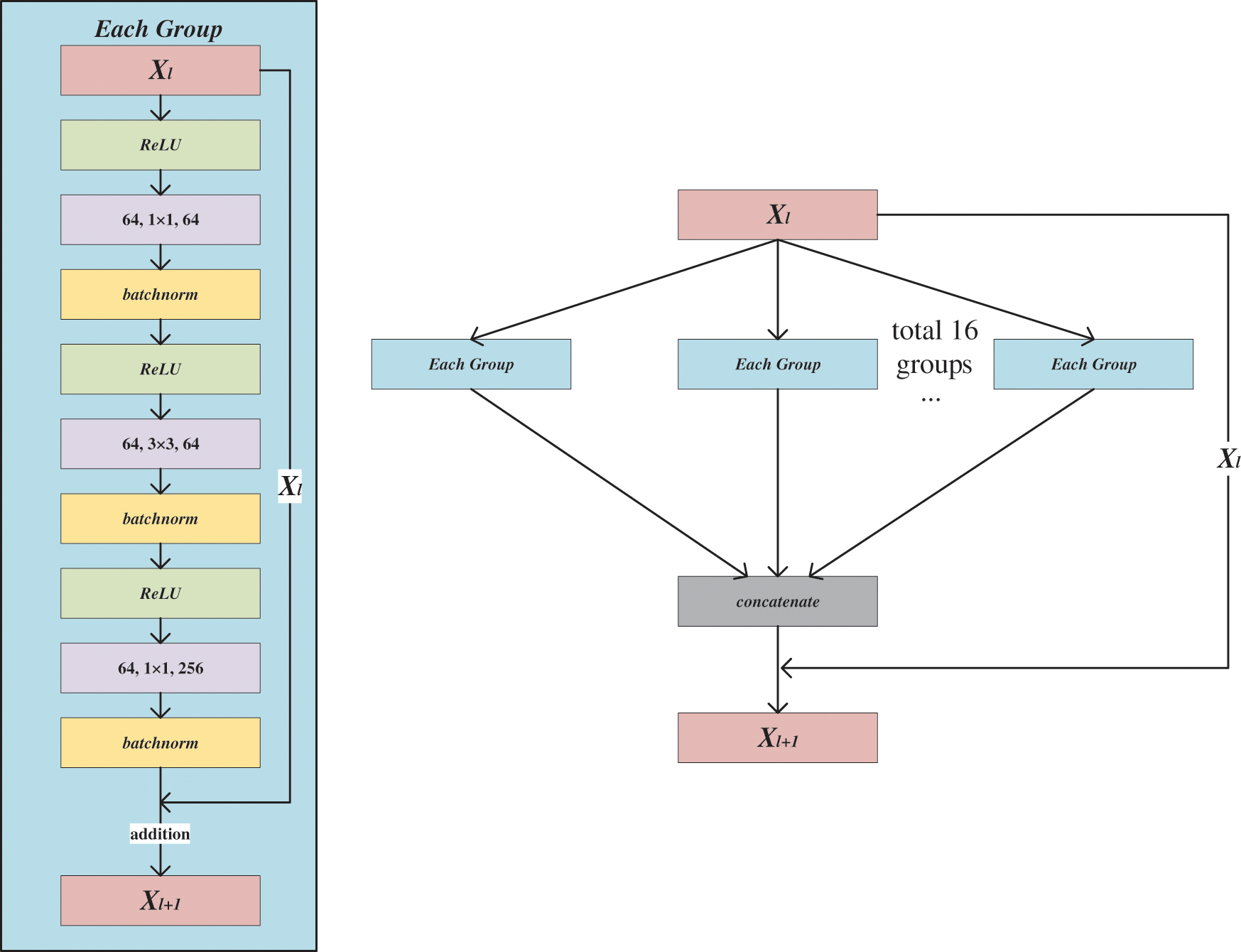
Figure 2: The architecture of the Pre-ReLU residual block

The output of the l th convolution layer is:

xjl=fl(∑i∈Mjxil−1×kijl+bjl). (6)

where xj is the i th output, fl(g) is the ReLU function, kijl is the convolution kernel, × means the convolutional multiplication, and the bias of this layer is bij.

The output of the M th pooling layer is:

xjm=fs(βjmS(xjm−1)+bjm). (7)

where the summation of the entire feature matrix is S(g), fs(g) means the SoftMax function, the weight coefficient is βj, the input for this layer is xjm−1, and the bias is bjm. By combining the Pre-ReNet with the loss introduced in the following subsection, we build a detector named B-PesNet. Then the architecture of our B-PesNet is shown in Fig. 3.

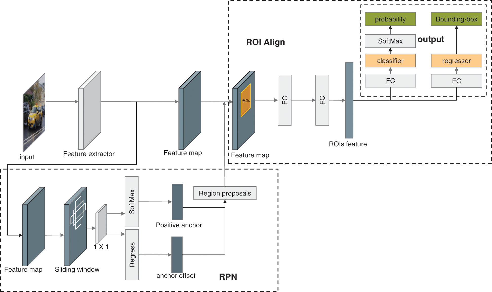
Figure 3: The architecture of B-PesNet

The input of the region proposal network (RPN) is a feature map, which is also used in the region of interest (ROI) Align layer. And the output of RPN is a set of rectangular regions named region proposals. We adopt the sliding window method to select a region titled anchor by sliding a window on the input feature map to obtain the region proposals. In each sliding window, multiple anchors are predicted simultaneously, and the maximum possible anchors of each pixel point are denoted by K . In this paper, K is set to 9 since there are 3 scales anchors, and each scale has 3 anchors with a different shape. Each anchor will be sent to SoftMax and classified it is positive or negative. At the same time, all anchors will perform a regress to get more actual coordinates. Then, the RPN will output the region proposals, which will be sent to the ROI Align layer. ROI Align reduces and normalizes those region proposals, extracts the ROIs feature vectors. And then, sends these vectors into the subsequent layer. The ROIs feature vector obtains the regression results and classification results through the Fully Connected and SoftMax layers.

The classifier and regressor in the output layer work are as follows:

Classifier: This layer will output the probability of objects in region proposals. The classifier will calculate the probability Pi of each element in the feature map i , which contains the object after thoroughly scanning the feature map.

Regressor: In this layer, the intersection of union (IoU) will be utilized to measure the accuracy of the bounding box (b-box). Then, the regressor will output the coordinates (x,y) of the center point of each anchor box, as well as the width w and height h of this box. IoU is calculated by Eq. (8):

IoU=A∩BA∪B. (8)

where A and B are the area of two region proposals.

Suppose the coordinates of the center point in the region proposal is (x,y), and the coordinates combined by width and height of this region proposal is (w,h). Then, a region proposal can be denoted by four indexes(x,y,w,h). Moreover, suppose (Px,Py,Pw,Ph), (GX,Gy,Gw,Gh), (Gχ′,Gy′,Gw′,Gh′), which are depicting the positive anchor, ground-truth box, and predicted box, respectively. IoU can be used to adjust the edges of the predicted box in regression progress. Assume the difference between the region proposal and ground-truth box is td=(tx,ty,tw,th), where:

tx=Gx−PXPw,ty=Gy−PyPh. (9)

tw=log(GwPw),th=log(GhPh). (10)

Then the loss function of the regressor can be written as:

Le=∑i=1N(tdi−ωdTϕ(Pi))2. (11)

here the ROI feature vector is ϕ(Pi), the coefficient achieved from the training phase is ωKT, the total number of samples is N , i means the i th sample. Thus, the classifier outputs 20k scores that denote the probability of 20 objects in the PASCAL VOC2007 dataset for each region proposal, the coordinates of k boxes are output by the regressor, which are 4k vectors.

3.4 Balance the Classes with an Improved Cross-Entropy Loss

The balanced loss (BL) is designed to handle the severe imbalance between foreground and background classes during the training phase, and the class imbalance overwhelms the cross-entropy (CE) loss. Quickly classified negatives cover the majority of the loss and dominate the gradient. Whereas, we propose to reshape the loss function to down-weight easy negatives, and then the network focuses on hard negatives during the training stage.

We introduce our BL starting from the standard CE loss:

CE(p,y)={−log⁡(p)if     y=1−log⁡(1−p)otherwise. (12)

here y∈±1 indicates the ground-truth class, and p∈[0,1] means the estimated probability of the model for the class with label y = 1 . For notational convenience, we define pt :

pt={pif     y=11−potherwise. (13)

then rewrite CE(p,y)=CE(pt)=−log(pt).

A common method to address the imbalance of classes is to introduce a hyperparameter. In our method, we introduce a weight coefficient α∈[0,1]. In our experiments, α shows the ability to balance the significance of positive/negative examples. Hence we write the BL as:

BL(p,y)={−αlog⁡(p)if     y=1−(1−α)log⁡(1−p)otherwise. (14)

Then both positive/negative examples will dominate the gradient while α< 1, For notational convenience, we define αt:

αt={αif     y=1−(1−α)otherwise. (15)

and rewrite BL to BL(p,y)=BL(pt)=−αtlog(pt).

The loss is a simple but effective extension to the standard CE loss, as our follow-up experiments show.

4  Data Processing and Evaluation Metrics

4.1 Data Processing

The data set trained, validated, and tested in this paper is the public dataset PASCAL VOC2007. It is composed of 21 classes, 20 foregrounds, and 1 back-ground.

Objects in real life are often under various interferences and are not as simple as the samples in the data set. A model trained with a simple data set will be challenging to apply to complex and changeable real-world scenarios, i.e., generalization is not strong. In order to overcome such a problem, online data enhancement operations will be introduced before training. Whether it is the human eye or the shooting device, it is possible to observe the object from any angle in the real world. The object might present a vastly different appearance due to the perspective. Accordingly, we warp the picture without changing the relevant information of the label. Twist operation can improve the generalization of the model in this respect. Besides this, there may be various interferences in the actual scene, such as intense light, haze, stains, etc. Therefore, we artificially highlight and blur the image to enhance the generalization of the model in such scenarios.

4.2 Evaluation Metrics

We utilize some common evaluation criteria to evaluate our detector in this paper. We utilize IoU, Precision, and Recall to evaluate our detector, and find the average of these experiments through multiple experiments and evaluations, which are

Precision=TP/(TP+FP), (16)

and

Recall=TP/(TP+FN). (17)

In Eqs. (16) and (17), TP indicates the number of samples for which the prediction is a positive example, which is a positive example. FP expresses that the prediction is positive, which is the number of samples for negative cases. FN represents that the prediction is negative, which is the number of samples for positive cases. Accordingly, Precision expresses how many of the predicted positive samples are genuinely correct, and Recall means how many of the predicted samples are genuinely correct.

mAP=1/C∑k=iN(k=i)NP(K)ΔR(k). (18)

In Eq. (18) [7], C represents the number of categories included in the model, N means the number of thresholds used as a reference, and k indicates the currently used threshold. P means the precision rate, R expresses the recall rate, and AP indicates the area under the precision-recall curve. The higher AP represents a better classifier. The average value of APs is mAP , where APs mean the sum of different classes. The value of mAP is within [0,1]. This index is the crucial index of the object detection algorithms.

5  Experimental Results and Analysis

5.1 Experiment Setup

We adopt VOC2007 as the training set and perform data augmentation, which adds artificial noise to each image. Moreover, we scale all inputs into the size of 224×224 to save calculation resources. We utilize stochastic gradient descent (SGD) with momentum as the optimizer with momentum as 0.9 and weight decay as 1e-4. All the experiments are performed on the same computer, and the main hard-ware settings are Intel® Core

TM

5.2 Calculation Results Using Different Backbones

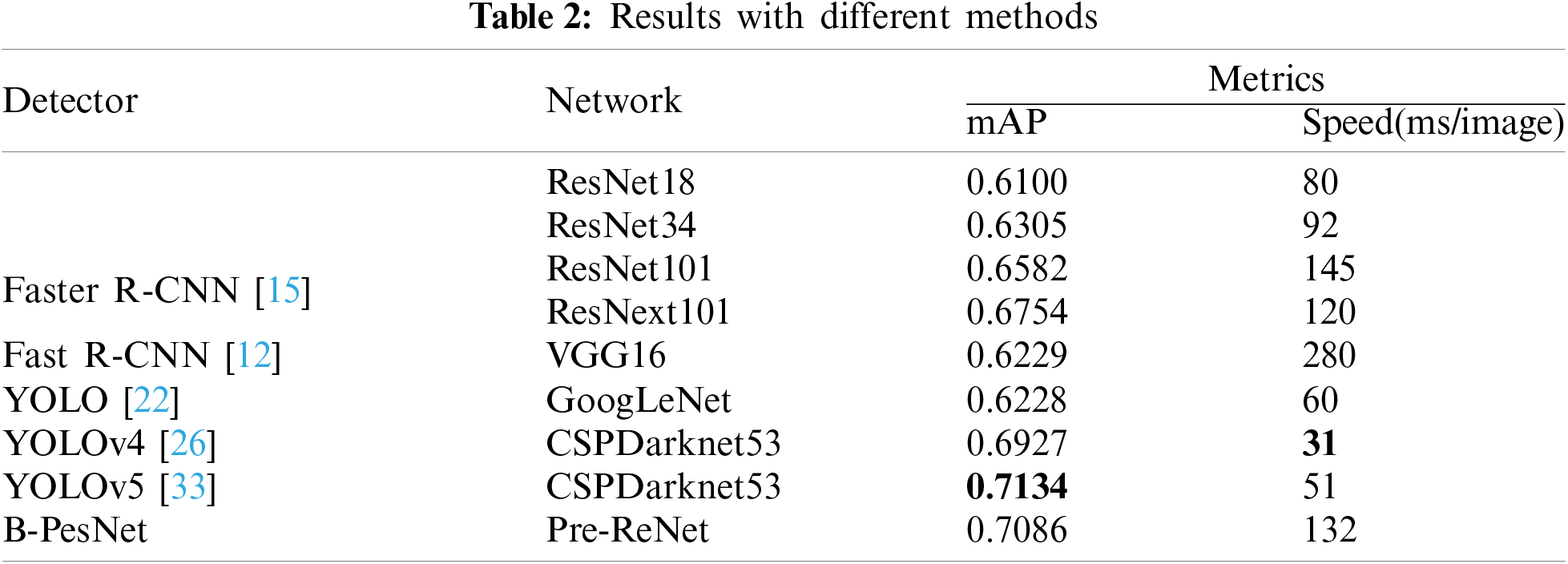
To test the impact of different backbones used in the detector, we have carried out experiments on different feature extractors to compare the difference of mAP. The mAP and calculating speed in the different condition is shown in Table 2. It is evident that the accuracy of our method is higher than the others except for YOLOv5. The accuracy of our proposed B-PesNet is inferior to YOLOv5 cause the network structure of YOLOv5 is more complex than B-PesNet. From this point of view, our B-PesNet is still valuable and meaningful. The B-PesNet obtain a balance between accuracy and speed.

5.3 Results by Different Detection and Recognition Approaches

To demonstrate the effect of the BL, we test some networks using BL or not. Table 3 shows the mAP for each condition. In this table, the value of α in every BL is 0.75. The reason for choosing 0.75 as the value of α will be discussed in subsequent sections. It is easily found that our BL is able to be inserted into any network as a plug-in. What is more, BL improves the performance of these methods. Furthermore, our B-PesNet is better than the other methods when using ordinary CE. The mAP of B-PesNet will increase to 73.34% while using BL as the loss function. The efficiency of the BL is shown in Fig. 4.

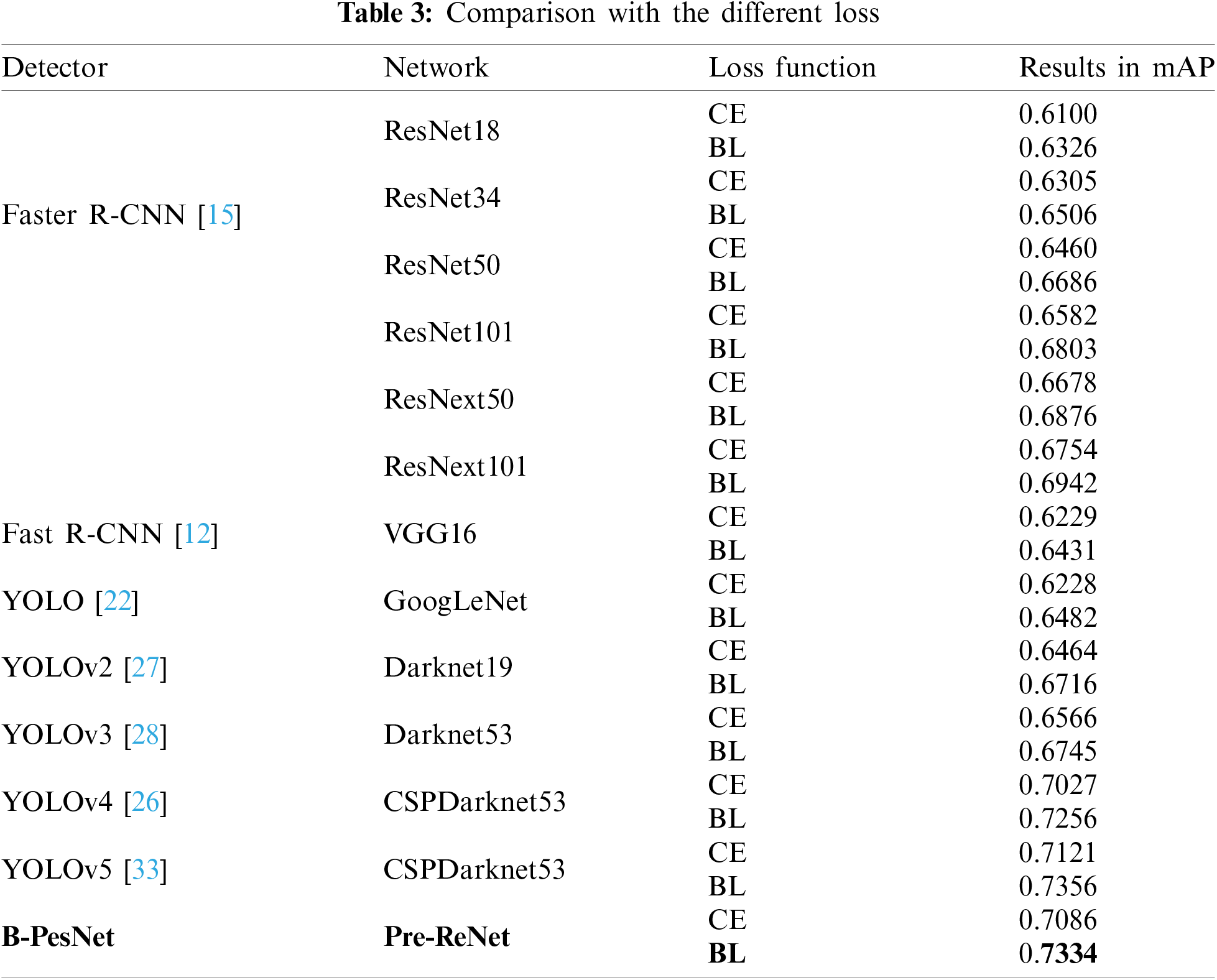
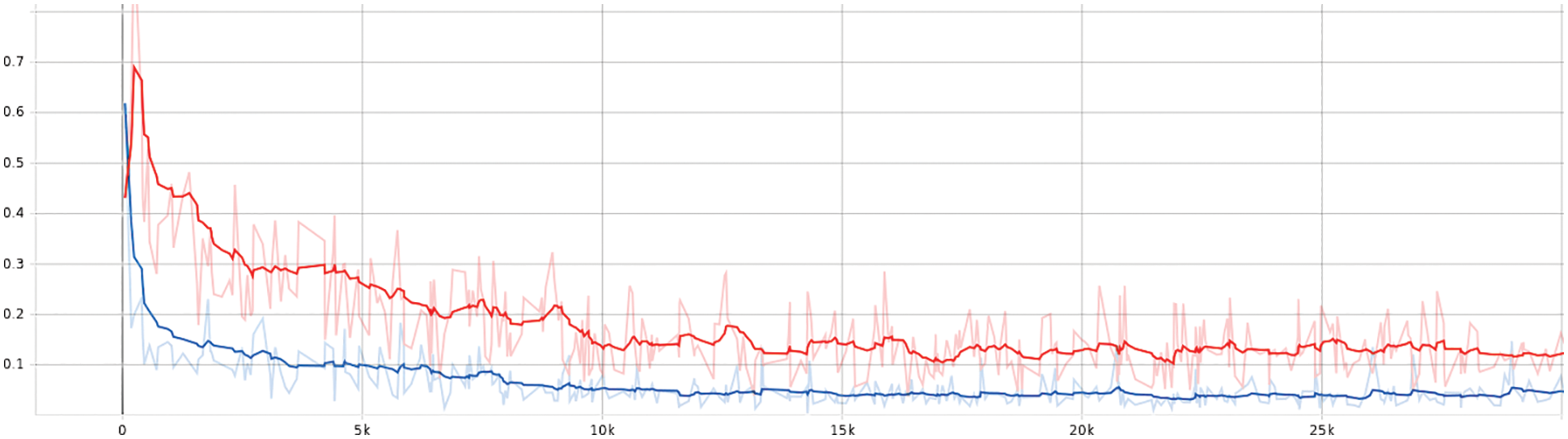
Figure 4: The loss curve of object classification. The blue one represents our B-PesNet with BL, and the orange one means our B-PesNet with CE. Obviously, the loss of B-PesNet with BL is lower and converges more quickly

5.4 Results by Using Different Hyper-Parameters

We chose 20 different values of α to verify the effect of the various hyper-parameter settings on BL performance. The result shows that when α is too small, the capability of BL will be inferior, even exacerbating the problem of class imbalance. When α is close to 1, BL will lose its effect and degenerate into ordinary CE. In this paper, we finally found that when α=0.75, the effect is the best. The experimental results are shown in Table 4.

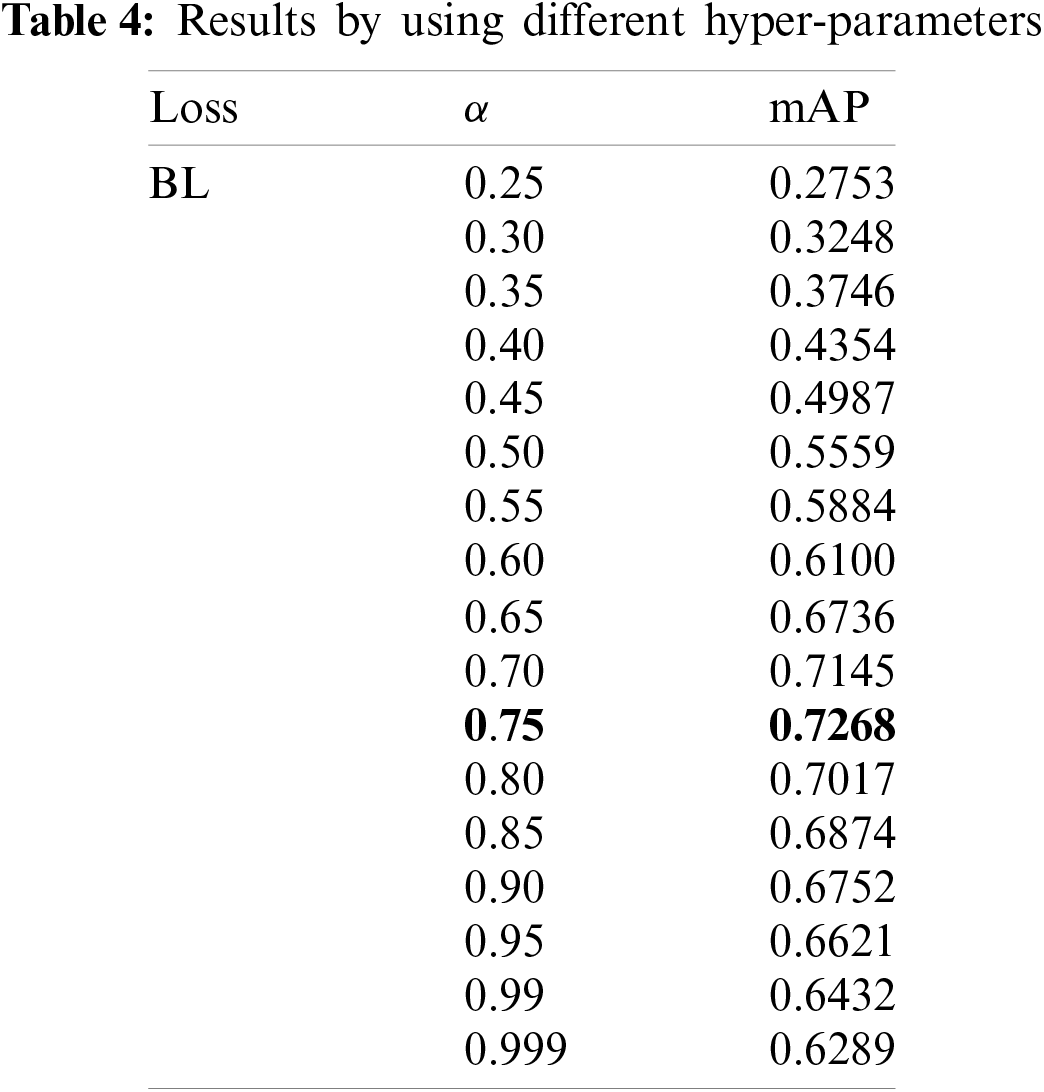
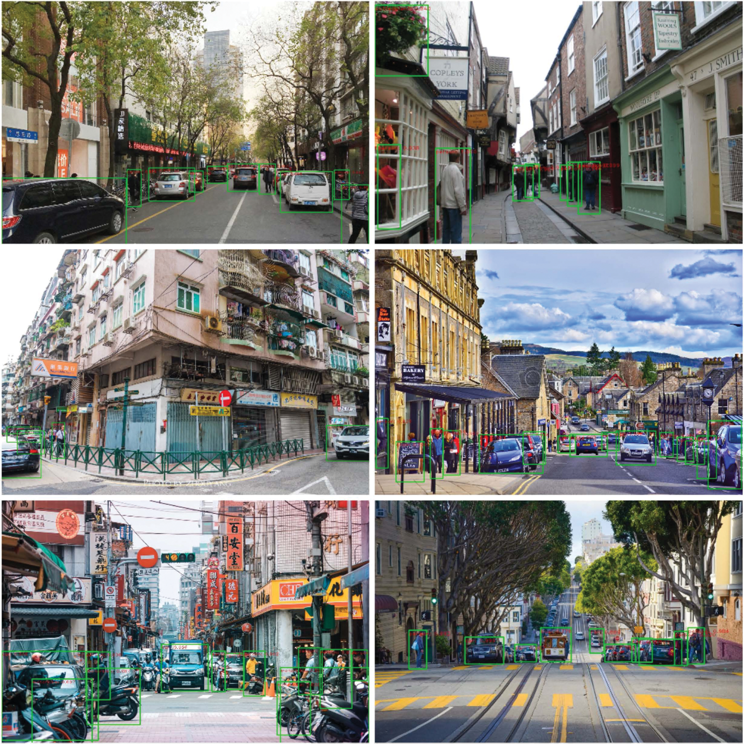
Figure 5: The detection results of B-PesNet. The detected target in the figure is marked by a green bounding box, and the mAP of the target is displayed on the upper part of the bounding box. The detection results of these actual scenes show that our B-PesNet has a good performance in a complex environment with interference factors such as occlusion and deformation

5.5 Results and Discussions

According to the results, we can infer that the semantic information is completely extracted, and the objects are accurately detected. From Table 3, it can be seen that our B-PesNet gets a balance between speed and accuracy. Table 3 shows that BL can tackle the class imbalance problem and improve the accuracy of the detector from the perspective of data. This shows that the research of deep learning can still start from data. As shown in Table 4, the parameters have a significant influence on BL performance. It is considering the definition of the formula, α should be set at a little larger value to have a better balance effect. Fig. 5 shows the detection results. In this way, we demonstrate that the new proposed loss plays an essential role in building a reliable detection for the security system.

6  Conclusions

We propose a method that improves the performance of the existing state-of-the-art two-stage object detection framework by enriching semantic information in shallow layers and introducing a new loss function, then demonstrate its effectiveness on the benchmark datasets. Our newly-designed network outperforms the previous neural network frameworks. The proposed B-PesNet shows above 1% mAP better than those typical object detectors. Compared with the existing approaches, the image processing speed of our method is also boosted. Greater efficiency imparts a higher practical value to the proposed method. This leads to a reliable solution for the applications of detection in security systems. In the future, we are interested in applying this detector to more specific scenarios, e.g., Internet of Things (IoT) applications in healthcare and health [36] and Blockchain-enabled IoMT [37].

Funding Statement: This research was supported by the Science and Technology Project of Sichuan (Nos. 2019YFG0504, 2021YFG0314, 2020YFG0459), and the National Natural Science Foundation of China (Grant Nos. 61872066 and U19A2078).

Conflicts of Interest: The authors declare that they have no conflicts of interest to report regarding the present study.

This work is licensed under a Creative Commons Attribution 4.0 International License, which permits unrestricted use, distribution, and reproduction in any medium, provided the original work is properly cited.