Computer Modeling in Engineering & Sciences

DOI: 10.32604/cmes.2022.019244

ARTICLE

Water Quality Index Using Modified Random Forest Technique: Assessing Novel Input Features

Wen Yee Wong1, Ayman Khallel Ibrahim Al-Ani1, Khairunnisa Hasikin1,*, Anis Salwa Mohd Khairuddin2, Sarah Abdul Razak3, Hanee Farzana Hizaddin4, Mohd Istajib Mokhtar5 and Muhammad Mokhzaini Azizan6

1Department of Biomedical Engineering, Faculty of Engineering, Universiti Malaya, Kuala Lumpur, 50603, Malaysia
2Department of Electrical Engineering, Faculty of Engineering, Universiti Malaya, Kuala Lumpur, 50603, Malaysia
3Institute of Biological Sciences, Faculty of Science, Universiti Malaya, Kuala Lumpur, 50603, Malaysia
4Department of Chemical Engineering, Faculty of Engineering, Universiti Malaya, Kuala Lumpur, 50603, Malaysia
5Department of Science and Technology Studies, Faculty of Science, Universiti Malaya, Kuala Lumpur, 50603, Malaysia
6Department of Electrical and Electronic Engineering, Faculty of Engineering and Built Environment, Universiti Sains Islam Malaysia, Bandar Baru Nilai, Nilai, Negeri Sembilan, 71800, Malaysia
∗Corresponding Author: Khairunnisa Hasikin. Email: khairunnisa@um.edu.my
Received: 11 September 2021; Accepted: 27 January 2022

1  Introduction

Water security is a rising global predicament at present. The scarcity of clean water could create a calamity of waterborne diseases around the world. Water pollution could conflict with agricultural and industrial output, which can lead to environmental degradation [1]. Factors that influence water quality include natural occurrences from the climate as well as anthropogenic inputs coming from untreated municipal waste, mining activities, industrial effluent discharges, sediment runoff, and land use changes [2,3].

Developed and developing nations across the world are constantly enforcing laws and reforming water quality management to improve sanitation and water quality status. The water quality index (WQI) has been commonly used as a universal indicator to convert several quantitative and intensive parameters into a single qualitative variable. Due to its simplicity, WQI is commonly utilized to describe the physical, chemical, and biological properties of water bodies. This representation of WQI is effective for water quality assessment and resource management [4].

In Malaysia, 90% of the nation’s water supply is derived from rivers and reservoirs. However, the per capita demand for water availability is growing at a rapid pace to support heavy manufacturing and large-scale crop cultivation. Population growth, improvement in living standards, and rapid urbanization have also imposed additional pressure on uncontaminated water resources [5]. According to statistics from the Malaysian Department of Environment (DOE) in 2017 [6], among the 477 rivers monitored in Malaysia, 47.0% were clean, 43.4% were semi-polluted, and 9.64% were polluted. In 1974, DOE adopted an ‘Opinion Poll WQI (OP-WQI)’ to rank the level of water quality. The panel of experts identified dissolved oxygen (DO), biological oxygen demand (BOD), chemical oxygen demand (COD), pH, ammoniacal nitrogen (NH3-N), and suspended solids (SS) as the utmost priorities [7].

In other countries, WQI models with various structures and weightings are developed by using sub-indexing and aggregation based on local opinions. The considered variables are inconsistent, since water pollutants such as heavy metals, pesticides, toxic compounds, and radioactive constituents are not included when evaluating water quality [8,9]. Most of the WQI models developed are region-specific, based on expert views and local guidelines, and many researchers have also highlighted the uncertainty of the WQI model [10–12].

Determination of water quality should be site-specific, with weightings decided according to water usage, taking into account such important parameters as phosphorus, nitrogen, trace metals, and fecal coliform. These variables are missing from the current Malaysian WQI assessment, making it less effective [13]. Malaysia’s WQI index only considers the use of common water quality parameters, hence leading to eclipsing problems. Eclipsing is where the true nature of water quality is not reflected due to inappropriate sub-indexing and aggregation functions [9].

The number of WQI parameters adopted in Malaysia is not flexible for the user and is independent of the natural and anthropogenic factors. Thus, this study aims to investigate the potential of other water quality parameters as input variables. The primary motivation of this study is to explore the possibilities of predicting water quality under the absence of six primary water quality input variables (DO, BOD, COD, NH3-N, SS, pH). To the best of the author’s knowledge, there is limited technical literature or research that focuses on predicting the water quality index using other water quality parameters. Hence, this study serves to fill the research gap of understanding the abilities of different water quality parameters in the assessment of water quality using a machine learning approach. The remaining sections of this paper are arranged as follows: Section 2 introduces the manual computation of the water quality index and reviews the research gap of existing modeling techniques using artificial intelligence. Section 3 outlines the area of study as well as the properties of the dataset. Section 4 presents the applied methodology for modeling and the proposed modeling schema. Section 5 discusses the modeling results and analysis of the input parameters. Section 6 ends the paper with a conclusion.

2  Literature Review

2.1 WQI Formulation

WQI is formulated from six monitoring parameters: dissolved oxygen (DO), biological oxygen demand (BOD), chemical oxygen demand (COD), suspended solids (SS), ammoniacal nitrogen (AN), and water acidity or basicity (pH). The formula involves subindex (SI) computation given in Table 1 before being fitted into the weighted formula in Eq. (1). Water quality is classified based on the Interim National Water Quality Standards for Malaysia (INWQS) shown in Table 2 [14]. Class I is classified as unpolluted and safe for drinking, Class II is fit for recreational and aquatic use yet requires conventional treatment, Class III is considered as polluted water supply and hence requires extensive treatment, Class IV is only for irrigation or domestic use, whereas Class V cannot be utilized for any purposes [15].

WQI=0.22SIDO+0.19SIBOD+0.16SICOD+0.16SISS+0.15AN+0.12SIpH(1)

Manual water quality calculation is lengthy, as it requires the process of converting raw data into subindex. Therefore, alternative techniques have been explored recently to provide a direct and simplified approach compared to the time-consuming computation process.

2.2 Machine Learning in WQI

River engineering to predict the ecological variables of water quality using artificial intelligence (AI) and machine learning (ML) is a widely recognized method to simplify the computation process of water quality assessment. Water quality parameters contain complex interactions and possess several nonlinear variables. AI techniques are adopted to understand the most suitable and efficient approach for modeling nonlinear inputs, evolving as a black-box model which brings environmental insights for strategic and planning purposes [16]. Various research works and technical literature are published based on the application of ML models such as neural networks, adaptive neuro-fuzzy inference systems, regression methods, ensemble techniques, and other hybrid models in water resource management [17–20]. These publications strive to understand the correlation of each water quality parameter, investigate the minimal number of inputs required for water quality index prediction, and spatially assess the point source and distribution of water pollution.

The most prominent tool for water quality modeling is artificial neural networks (ANNs), as the outcomes delivered from ANNs are consistently high in accuracy. ANNs are remarkable at forecasting and identifying problem variables from a set of complex or inaccurate data. When it comes to estimating WQI using ANN, the use of backpropagation neural networks (BPNN) and radial basis function neural networks (RBFNN) is equally effective for simplifying the computation process of WQI in the Langat and Klang Rivers, Malaysia [21]. The parameters used for the work in [21] are based on DO, BOD, COD, NH3-N, SS, and pH, with the best coefficient of determination (R2) evaluated using RBFNN at 0.9807 when BOD is excluded from the input. The authors ranked DO as having the highest correlation with WQI. Othman et al. [15] constructed an ANN model of 98.78% accuracy as the basis of water quality assessment. The publication benchmarked that the best performance was attained when only five input parameters were considered, eliminating pH as an input variable. Nevertheless, ANNs are prone to overfitting and facing local minima problems [22], though these shortcomings could be overcome with optimization and generalization techniques.

Tiwari et al. [23] explored the capability of an adaptive neuro-fuzzy inference system (ANFIS) by predicting WQI based on two clustering techniques, fuzzy C-means (FCM) and subtractive clustering (SC). The model’s performance was significantly close to the experimental value, and it suggested ammonia, chlorides, and fecal coliform as the most sensitive parameters for water quality assessment in India. Multistep modeling performed by Elkiran et al. [24] compared several AI models, i.e., BPNN, ANFIS, support vector machine (SVM), and a linear autoregressive integrated moving average (ARIMA) model, in DO prediction. The authors explained that ANFIS might have better verification in two of the three stations evaluated, while SVM has an edge in prediction performance in one of the stations. Abobakr Yahya et al. [25] developed an SVM approach for ungauged catchment water quality prediction; the presented model proved to be efficient, with high precision, yet sensitive to the error level.

2.3 Research Gap in WQI Modeling

In summary, based on the above literature, it is evident that water quality prediction models based on machine learning are reliable and capable. It is also apparent that the determinant features of water quality vary according to the area of study, since different rivers have different land use purposes, and hence, certain water quality parameters may seem significant for a specific river but not be universally applicable. Although the application of AI models to water quality assessment has significantly increased, many models merely consider input parameters from the water quality index formula. Meanwhile, other water quality parameters and their role in water quality assessment have yet to be explored. There are approximately 30 water quality parameters, which include biological, chemical, and physical parameters, as well as trace metals of water bodies that interact with each other and affect water quality. However, there is a lack of critical parameters in most WQI models [9]; for example, the Malaysian WQI only considers common WQ inputs, neglecting biological indicators.

Moreover, the influence of land use, human activities, and socioeconomic behavior have different effects on the variability of water quality. The hydrological process of rivers is dynamic and complex; hence, it is mandatory to understand other significantly influential variables that have nonlinear processes in water quality assessment. This information is essential as a way toward formulating water quality in terms of adaptive parameters that suit the land use activities around the river.

The existing development of water quality modeling had the following research gaps: (1) Existing publications are focused on comparative analysis of different AI techniques and approaches, aiming at simplifying the WQI calculation process; the current WQI was limited to just six water quality parameters, so other water quality parameters were not taken into consideration. Models should be updated when new data or evidence is found about what is polluting the water source. (2) Sensitivity analysis from research articles [15,21,26] has continuously concluded that among the six water quality input variables, certain variables can be omitted, thus suggesting the possibility to investigate more water quality aspects for water quality assessment and management. (3) Change in anthropogenic activities in the 21st century has had an impact on water quality exposure, hence the rising need to redefine important water quality variables as input parameters.

3  Materials and Methods

3.1 Study Area

The two rivers considered in this research study are the Klang River and the Langat River (Fig. 1); most of the rivers in both river basins are in the semi-polluted and polluted categories within the Federal Territory of Kuala Lumpur and state of Selangor, Malaysia. The two main rivers supply hundreds of thousands of people in the Klang Valley. Therefore, consumers were highly affected when wastewater treatment plants were forced to shut down due to water pollution. Hence, there is an arising need to monitor the health of both rivers, as they are important water sources for domestic use.

Figure 1: Klang river and Langat river at Selangor, Malaysia

The Klang River is approximately 120 km in length with a basin area of 1288 km2, located at 2°55′N–3°25′N latitude and 101′I5′E–101°55′E longitude. The upstream begins in the mountains of Peninsular Malaysia at 1200 m altitude, comprising the Gombak and Hulu Langat districts, running through the heart of Kuala Lumpur, then crosses part of Selangor state before stemming with Port Klang to the Straits of Malacca. Most of the river basin is surrounded by urban infrastructures and industrial, recreational, and residential utilities. The river lies in a tropical climate area with heavy rainfall during the Southwest and Northeast Monsoons, average monthly humidity of 80%–85%, and uniform temperature between 27°C and 31°C. The area receives daily sunshine for 4.5 to 7.0 h per day, with an evaporation rate ranging between 3.0 and 5.0 mm daily [26,27]. The water quality of the Klang River basin is deteriorating due to the combination of rapid urbanization and high occurrences of pollution. Based on Sharif et al. [28], among the sources of pollution are residential and industrial runoff from construction sites and sewage discharge from treatment plants. It is estimated that 77,000 metric tons of garbage are dumped into the Klang River every year.

Meanwhile, the Langat River stretches across a total catchment area of 1815 km2 across Kajang, Cheras, Bangi, and Putrajaya, situated between latitudes 2°40′M 152″N and 3°16′M 15″N and longitudes 101°19′M 20″E and 102°1′M 10″E. The main river is 141 km long, located 40 km to the east of Kuala Lumpur, featuring large tributaries such as the Semenyih River, the Lui River, and the Beranang River. The river flows from a highland altitude of 1500 m at the Pahang–Selangor border, draining towards the Straits of Malacca. The Langat and Semenyih Reservoirs are built for domestic and industrial water supplies and to generate power for Langat Valley. The Langat River also supports numerous activities such as effluent discharge, irrigation, fishing, and sand mining along its streams. The catchment also serves as an important water source facility to 1.2 million people [25,29].

3.2 Data Collection and Monitoring Sites

The dataset used for this study was obtained from the Department of Environment (DOE), Malaysia at 94 monitoring stations (shown in Fig. 1) along the Klang and Langat Rivers during the period between 2014 and 2019. The water quality parameters that are included in this study are DO, BOD, COD, NH3-N, SS, pH, conductivity (COND), salinity (SAL), turbidity (TUR), dissolved solids (DS), nitrate (NO3), chloride (Cl), phosphate (PO4), Arsenic (As), Chromium (Cr), Zinc (Zn), Calcium (Ca), Iron (Fe), Potassium (K), Magnesium (Mg), Sodium (Na), E. coli, and total coliform. The type of pollution for both the Klang and Langat Rivers is similar, as both areas are located in densely populated industrial and residential districts; given the average similarity of the data analyzed, both datasets were merged, and the statistical properties of each river are compiled in Table 3 below.

The distribution of DO in the Klang River ranged between 0.50 mg/l and 11.51 mg/l, with an average of 5.4 mg/l; a significant fraction of DO values fall in Class III. As compared to the Langat River, which has an average DO of 6.0 mg/l, the Klang River is much more deprived of dissolved oxygen to sustain aquatic life. Both rivers have a mean DO value of 5.49. Pollution in the Klang River is much more evident, as BOD and COD levels are in Class IV (10.59 mg/l) and Class III (32.47 mg/l). The Klang River is at serious ecological risk, as the mean value of NH3-N is categorized in Class V at 4.28 mg/l.

The pH value, on the other hand, is in Class I, similar for both the Klang and Langat Rivers at an average of 7.34 and 7.31, respectively. The concentration of SS in the Klang River is under control in Class II, with a mean of 35.05 mg/l, whereas the SS concentration in the Langat River demands more attention, as it is in Class III (115.22 mg/l). The BOD and COD concentration of the Langat River are in the same class as the Klang River; ammonia levels, averaging 2.0 mg/l, fall into Class IV.

Throughout the monitoring period, the Klang River was classified as Class III 56.7% of the time, and 62.2% of the Langat River’s data are categorized as polluted in Class III according to the WQI index. The distribution of WQI for both rivers is illustrated in Fig. 2. The WQI classification of the entire dataset has the highest percentage in Class III (57.42%). Overall, only a fraction (28.75%) of WQI data are in Class I (2.72%) and Class II (26.02%). There are a total of 759 instances where the water was unfit for any purpose.

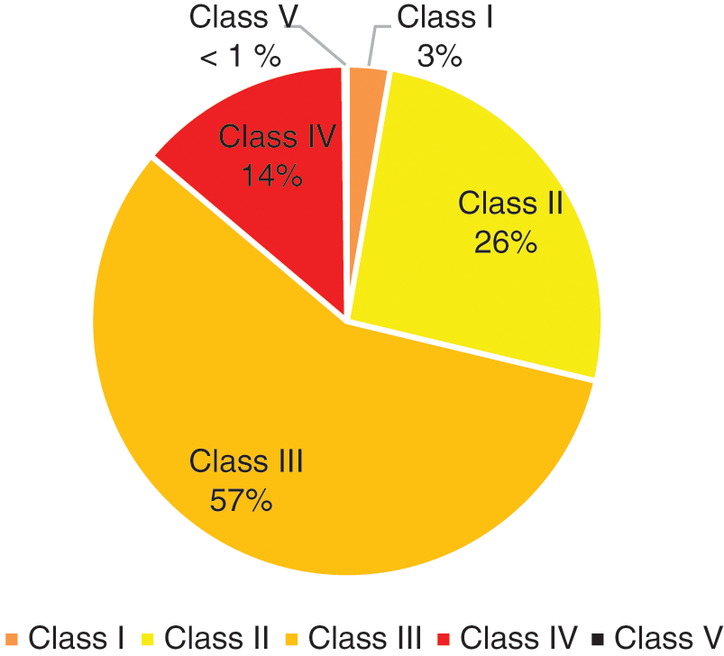
Figure 2: Class distribution of water quality in Klang and Langat River for n = 5,483 samples

The variability of samples is largely due to the geographical variation of pollution sources dispersed into the river basin. Both rivers flow through urban areas and townships where wastewater or sewage effluent is poured into the river channels. For example, significant variation can be observed in turbidity, as the maximum value is 3529 NTU and the lowest is 0.00 NTU. The large variation could be the impact of industrial effluents and urban runoff mixing from water treatment processes.

4  Methodology

The major goal of this study is to propose a prediction model that predicts WQI using a new set of features instead of the conventional features that are usually applied in the WQI formula. Therefore, the six common WQ variables (DO, BOD, COD, NH3-N, SS, and pH) were not included in the modeling process. Instead, new water quality features are applied in this work, including COND, SAL, TUR, DS, NO3, Cl, PO4, As, Cr, Zn, Ca, Fe, K, Mg, Na, E. coli, and total coliform. The methodology of this study is illustrated in Fig. 3 below, which involves data preprocessing of the dataset, followed by preliminary model selection using five machine learning regression algorithms. This step acts as the data analysis stage to select a suitable model capable of predicting WQI with the 17 input features. Next, the best-fitting algorithm is chosen for classification training. In the training phase, two sets of training data are applied; the first set is the unmodified training data, which contain imbalanced classes, while the next set of training data is modified using the data augmentation technique. The synthetic minority oversampling technique (SMOTE) is an oversampling approach to recreate synthetic examples of minority classes [30]. The results are then analyzed based on the accuracy, precision, recall, and confusion matrix. Lastly, sensitivity analysis was carried out to evaluate the relative importance of the 17 new input parameters among all 23 input parameters.

Figure 3: The proposed methodology

4.1 Preliminary Model Selection

Regression algorithms are suggested in this study as a data analysis step for choosing an algorithm that could predict the continuous values of WQI. The regression technique is a supervised machine learning algorithm that allows the prediction of a continuous outcome from one or more predictors. The basis of this technique often involves modeling the relationship and dependencies between the target output and input features to predict the value of a given new datapoint. The following five machine-learning algorithms are employed in this study.

4.1.1 Multilayer Perception

Multilayer perception (MLP) is a variant of the classical ANN model, popular for both classification and regression. MLP models operate on a network of sigmoid activation neurons connected by links of several weights. The three basic layers of the MLP model consist of the input layer going through hidden layers to reach the output layer [31].

The net input Neti is the addition of the threshold bi with the summation of input values x (xi to xj) multiplied by assigned weights w (wi to wij). The weights represent the strength of each neuron, which is optimized throughout the whole training process.

Neti=bi+∑j=1nwijxj(2)

The activation function then accepts the input from the previous layer and transfers the output to the next layer [29].

f(Neti)=11+e−Neti(3)

4.1.2 AdaBoost

Adaptive boosting (AdaBoost) is an ensemble learning-based model that combines multiple base learners, which generally outperform a single learner. The AdaBoost regression can automatically adjust the weightage of the model based on estimation errors by generating multiple regressors [32]. It has the potential to enhance the generalization capability of nonlinear and complicated regression problems [33].

4.1.3 Support Vector Regression Machine

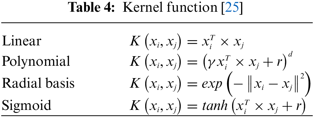
Support vector regression machines (SVRMs) are a generalization of support vector machines to estimate the continuous output value. SVRMs are widely known in pattern recognition and regression problems due to their generalization principle adopted from the structural risk minimization theory (SRM), which minimizes the empirical risks of overfitting in statistical learning theory [34]. The development of SVR models is aimed at reducing the upper bound error, where the four main kernel functions of the SVR model are the linear, polynomial, radial basis, and sigmoid functions [35].

The value of the kernel function K(xi,xj) is equal to the inner product of two vectors, xi and xj. The common kernel function types are shown in Table 4, where γ, r, and d are kernel parameters.

4.1.4 Decision Tree Regression

Decision tree regression (DTR) is a popular machine learning tool used in event outcome prediction, investment risks, and decision-making. Decision trees classify instances based on feature values, starting from the root node. The instances are represented with nodes, and each branch in the decision tree holds a value that the node can assume [36]. The decision tree model applies a top-down, recursive divide-and-conquer mode. After the feature of the root node is selected, the branch of each feature is given possible values, and this process is repeated recursively until all instances contain the same class. The decision tree approach is useful in predicting unpredictable outcomes by adding new scenarios into the complex dataset until a behavioral pattern is found [26]. The DTR algorithm extracts the features from the dataset, organizes the features into a tree-shaped structure, and combines a series of basic rules in the prediction stage [17].

4.1.5 Random Forest

Random forest (RF) is an ensemble learning algorithm that can be both a classification and a regression method. The RF creates several decision tree predictors that were initially uncorrelated from the sample dataset and assembles these weak learners into a strong learner [37]. The training data are randomized into a few samples and formed into several tree predictors. The RF algorithm shown in Fig. 4 generates results based on the average result of each tree [38,39].

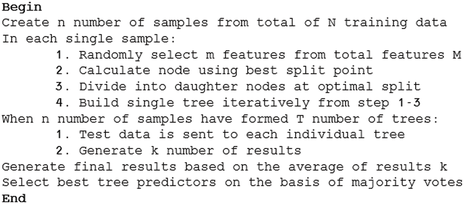
Figure 4: The random forest pseudocode applied in this work

4.2 Regression Evaluation

In order to evaluate the goodness of fit of the trained algorithms, four statistical measurements are applied to analyze the performance of the RF, AdaBoost, DTR, SVR, and MLP-NN models. The performance metrics applied are the mean absolute error (MAE), mean squared error (MSE), root mean squared error (RMSE), and the coefficient of determination (R2). MAE is often used to represent the discrepancy of error expected from the forecast on average, it is the average absolute difference between observed and predicted outcomes. Meanwhile, MSE and RMSE represent the squaring or square root of the computed error. Both measures are disproportionate to the actual increase in error. The R2 metric measures the proportion variation of the outcome estimated by predictor variables. In regression models, R2 is the squared correlation between observed and predicted values. A higher R2 and lower MAE, MSE, and RMSE values present better fitness and smaller discrepancy. These statistical measures are calculated based on the following formulas:

MAE=∑i=1n|yi−y^1|n(4)

MSE=1n∑i=1n(yi−y^)2(5)

RMSE=1n∑i=1n(yi−y^)2(6)

R2=1−∑i(yi−y^i)2∑i(yi−y¯)2(7)

4.3 Classification Training

Classification training refers to models’ learning to categorize class labels based on the input data. The classification models assign label values and separate new observations into a specific class. In this study, classes are generated from the WQI ranges provided in Table 2. Discrete categorical data are converted from the continuous WQI values based on the index range. There are a total of five classes with Class III as the majority class, while Class I and Class V have a limited number of observations. This section of the study includes the methodology proposed for addressing the case of an imbalanced dataset.

4.3.1 Synthetic Minority Oversampling Technique (SMOTE)

An imbalanced dataset occurs when the dataset contains classification categories that are not equally represented. Imbalanced datasets are commonly handled by using oversampling or under-sampling techniques. SMOTE is a feasible approach for oversampling the dataset with recreation of synthetic samples for the minority class [30]. The new data are sampled along the line segments joining k minority class samples based on interpolation (Fig. 5).

Figure 5: An illustration of the SMOTE interpolation of a selected minority sample, extracted from Douzas et al. [40]

4.3.2 Classification Evaluation

Several performance metrics are applied in the evaluation of the classification models. The confusion matrix is used to show information between the actual and predicted values performed by the classification system by means of true positives (TP), true negatives (TN), false positives (FP), and false negatives (FN). A common measure of classification performance is prediction accuracy, which shows the proportion of the total number of correct predictions against the total number of the testing dataset.

Accuracy=TP+TNN×100%(8)

where N is the total number of testing data.

Precision, recall, and F1-score are also calculated to evaluate the effectiveness of the classifiers. Precision measures the ratio of correct positive class predictions to the total predicted positives. Recall or sensitivity quantifies the ratio of correct positive class predictions to the total positive observations. The F-measure is a score balancing between precision and recall. Ideally, measures closer to one show the best performance.

Precision=TPTP+FP(9)

Recall=TPTP+FN(10)

F1score=2×Precision×RecallPrecision+Recall(11)

4.4 Sensitivity Analysis

Sensitivity analysis is the assessment of the importance of each input variable in the fitted model. The analysis is based on the ‘leave-one-out’ method, where changes in network error are recorded. The analysis performs parameter ranking according to the ratio of the leave-one-out model with the reference model. The results of sensitivity analysis often provide useful information on the effects of each predictor, which is insightful for pruning input parameters [7].

In this study, two sensitivity analyses are carried out to compare the rankings of all 23 parameters with the 17 new parameters. The method computes the misclassification rate when each variable is removed. The ratio of each variable is then calculated based on the error of the reduced model against the full model. A higher ratio returns higher significance of the parameter in the system.

5  Results and Discussion

5.1 Input Variables and Data Processing

A total of 5,483 samples of water quality parameters were obtained after pre-processing of the dataset received from the Department of Environment. Features such as E. coli and dissolved solids have very wide scales and distributions, which may lead to inaccuracy and degradation of the predictive performance, specifically algorithms that incorporate dimensional or distance elements. Hence, data normalization is applied to the dataset by setting the minimum and maximum threshold to be between [−1, +1]. To ensure each water quality variable has equal bounds in the analysis, the dataset is fit into a mean of zero and a variance of one.

Next, the water quality index (WQI) is calculated based on Eq. (1) and classified into five classes shown in Table 2 and Fig. 2. Split validation is used in this study by splitting the data into two groups: 80% for training and 20% for testing.

The correlation coefficient between input variables for the Langat and Klang Rivers is depicted in Table 5. It is apparent that salinity, DS, Cl, Ca, K, Mg, and Na are significantly correlated with conductivity at r > 0.8. A high positive correlation is also observed between Na and K (r = 0.92), which in turn are at r = 0.97 and 0.96 with Cl, respectively. The hardness of water could also be represented by the good relation between Ca and Cl (0.80). These values show the influence of ion concentration on the salinity and conductivity of the river.

The highest negative correlation is found between NO3 and As (−0.04), and between Fe and K (−0.04), Mg (−0.03), and Na (−0.03). The presence of E. coli and total coliform has no effect on other water quality parameters, while both are closely related at r = 0.62.

5.2 Preliminary Model Selection

In this study, the Python programming language is used for data pre-processing and the prediction model. The scikit learn packages are applied to select the appropriate model for the prediction analysis. Five machine learning models are trained to predict WQI based on 17 input parameters, and the performance is shown in Figs. 6a–6e below. Based on the simulated and observed WQI for 20 sample data, it is evident that despite excluding the conventional six input parameters used to formulate WQI, the new 17 input variables are competent in achieving close prediction for WQI in most of the prediction models.

Figure 6: Comparison of the observed and simulated WQI using (a) random forest, (b) AdaBoost, (c) decision tree regression, (d) support vector regression, and (e) multilayer perception

The DTR model showed the highest fluctuation pattern and was unable to capture the pattern of the WQI accurately. Even though the AdaBoost model was able to reach exact predictions for a few of the datapoints, the model showed high deviation from the actual value for most of the samples. On the other hand, both SVR and MLP models are good at modeling the WQI, since several simulated values are in line with the observed values. Apparently, the RF model has better prediction performance, given its higher accuracy in simulating WQI compared to the other models. The RF model is better at simulating the pattern of the observed values.

Table 6 presents a comparison of performance metrics’ evaluation between the trained models. The results indicate that in most of the simulated WQIs, the RF model predominated, with the highest R2 and a fair RMSE. The weakest performance was associated with the SVR model, for which the performance metrics have higher mean errors in both datasets. The AdaBoost, DTR, and MLP models produced average results compared to the other methods.

The obtained RMSEs for RF, ADA, DTR, SVR, and MLP are 2.425, 7.173, 6.382, 7.915, and 7.241, respectively. The RF model provides the smallest RMSE, MSE, and MAE among the other algorithms, which confirms the capability of the RF model to predict WQI. The reason RF outperforms the other models is its capability of learning nonlinear relationships between the WQI and input layers. Random forest possesses higher robustness in handling outliers and unbalanced datasets, as it is efficient in decreasing bias and overfitting of data [41]. Thus, the overall results show the superior performance of RF models with the input combination COND, SAL, TUR, DS, NO3, Cl, PO4, As, Cr, Zn, Ca, Fe, K, Mg, Na, E. coli, and total coliform. All five techniques were compared to the actual outcome, plotted in Fig. 7. The results suggest that the RF regression method provides better predictive accuracy in terms of all performance evaluation parameters. The pattern of the plot obtained portrays the linearity of the algorithm, which has moderate accuracy. The substantial improvement in the predictive accuracy of the RF approach using the alternative set of input features indicates that it can be effectively used in predicting the impact of water quality.

Figure 7: Correlation between the observed and simulated WQIs using (a) random forest, (b) AdaBoost, (c) decision tree regression, (d) support vector regression, and (e) multilayer perception

5.3 Classification Training

As per the investigation conducted in 5.2, the RF model is proven competent in modeling the behavior of the 17 water quality inputs, which correspond to the continuous WQI output. This section of the study performs classification modeling of the five WQ classes shown in Fig. 2 using a random forest classifier. The study aims to improve the efficiency of classification prediction through a modified training approach. Two RF classification models will be tested on two different datasets: Model A is trained on Training Set A, which contains an unmodified training dataset, and Model B is based on the SMOTE-modified Training Set B. Models A and B are then tested on a new testing set, and both models’ performance is then compared in terms of their confusion matrix, accuracy, precision, and recall, tabulated in Table 7.

The recall rate (Table 7) shows that the sensitivity of Model A towards Class V is the worst. This is critical, as dangerous water that is incorrectly classified could be consumed. An improvement in recall is seen in Model B, with a 75% sensitivity rate. Moreover, the precision and recall rates of Class I also improve from 33% to 54% and 10% to 48% when Model B is trained with the SMOTE modified training dataset. However, the accuracy of Model B is much lower, as Model B’s performance in predicting Classes II and III shows a decline. This is possibly due to the training process of SMOTE—the presence of indistinguishable boundaries between the two classes introduces noise to the model [40]. Nonetheless, Model B has the best performance in average F1-score as compared to the unmodified Model A. In the case of water classification, precision and sensitivity are the most important estimates. In Fig. 8, class-wise accuracy is represented in the form of a confusion matrix. Fig. 9 provides a visual overview of the classification performance of Model A and Model B. Significant improvements are observed for predictions of Class V and Class I. Overall, the accuracy of both models is substantially similar in agreement, at 79.66% for Model A and 77.68% for Model B.

Figure 8: Confusion matrix for WQI classification of random forest (a) Model A, (b) Model B

Figure 9: Visual comparison of the precision, recall, and F1-score between Model A and Model B

5.4 Sensitivity Analysis

The results of sensitivity analysis among the 17 and 23 input variables (Table 8) highlight the importance of certain water quality variables that are not present in the current WQI formulation. The rankings from Table 8 show turbidity as the first determining factor for predicting WQI with unconventional features. The firm ground of turbidity’s importance was also proven when the 23 predictors were analyzed. Turbidity ranked as the sixth parameter, while the first five parameters were the conventional input features. The common input feature pH shows less significance in this study as the 13th variable. Moreover, sensitivity analysis also shows that the variables sodium, chloride, and conductivity were less influential in both WQI predictions. These variables could be removed from the future experimental phase to provide better generalization and less noise for the model.

5.5 Discussion

The significance of unconventional water quality variables has been constantly published in research materials that highlight the absence of COND, DS, Cl, Na, Cl, As, Zn, Fe, and other heavy metal concentrations such as aluminum (Al), cadmium (Cd), chromium (Cr), and lead (Pb) from drinking water quality standards [42]. Results from Wagh et al. [43] also further showed that groundwater is constantly saturated with pollutants such as COND, Na, Cl, and DS which exceeded the desirable limits. Areas that are affected by urban land use activities often have COND, NO3, PO4, Cl-, DO, BOD, Pb, Cd, and total coliform values above the stipulated standards [44].

Therefore, it is evident that alternative water quality parameters should be included in assessing water quality. The hypothesis is proven in this study that these inputs will contribute towards accurate prediction of water quality. Although none of the inputs used were part of the conventional WQI subindex’s formula, the proposed modified RF model managed to achieve a coefficient of determination of 0.974 and error below 6%. The proposed model indicates that 97.4% of the variability of WQI can be explained by the 17 water quality inputs. Nonetheless, a modified approach is required when handling the classification of the dataset. From Section 5.3, it is evident that the proposed integration of SMOTE with RF could improve the real positives predicted.

The findings from this study correspond to previous works tabulated in Table 9, which shows that the proposed modified RF model is efficient in WQ modeling. The adoption of SVMs in [45] suggested that, if the least relevant parameters are included, the SVM model has less advantage in prediction. This is also proven in this study, as the SVR model showed R2 of only 0.69. On the other hand, Ho et al. [26] conducted a leave-one-out analysis on all six common parameters and concluded that exclusion of DO, BOD, and COD had a large impact on accuracy. Sensitivity analysis by Gazzaz et al. [7] pointed out that, for the Perak River, DO, BOD, NH3-N, pH, COD, and turbidity should receive priority in WQI computation instead of using SS. The research ranked SS concentration 18th in importance, while the WQI ranked SS concentration third.

In summary, the use of other WQ parameters should not be entirely neglected when assessing WQI. The WQI formulation should be tailored according to the river’s needs. Besides that, a suitable machine learning model as suggested in this work is important to model the nonlinear inputs.

The use of the proposed new water quality variables is beneficial because most of the water quality parameters are interrelated. In the published work by Joarder et al. [46], electrical conductivity was analyzed as one of the most appropriate variables to justify most of the dependent variables for WQI. Electrical conductivity is also directly related to the content of DS and salinity, where a high electrical conductivity signifies a significant number of impurities present in the water source. Commonly, the impurities consist of ions such as chloride, phosphate, and nitrate from sewage runoff and agricultural waste. Chloride content dominant in water content could cause corrosion of iron plates or pipes [47]. Excess nitrate and phosphate concentration is toxic to human consumption and could stimulate algal blooms that would cause oxygen depletion or eutrophication [48]. However, previous works only considered DO in the WQI formulation to represent these reactions, which can be considered inadequate and less robust.

Moreover, the measure of turbidity is also influential in predicting WQI yet neglected by the conventional WQI formula. Turbidity describes the clarity of water, where high turbidity represents a dense mixture of clay and organic matter. The presence of these foreign compounds directly affects light transmission to aquatic plants; hence, lowered photosynthesis would result in lower dissolved oxygen and unfavorable water quality [49]. In addition, the potential risk of heavy metal contamination originating from water sources was also found to affect the mangrove forests of Kuala Selangor [50] and the Klang estuary [51]. Since these metal concentrations are not present in the conventional WQI measurement, the estuary ecosystem is unknowingly still being fed from heavy metal–contaminated water sources even though WQI is continuously monitored.

Nevertheless, despite the high compliance of the RF model in modeling the nonlinear relation of these inputs, the simulation model could be improved through optimization algorithms to reduce the errors. The high average magnitude of errors is because the target WQI does not include any of the proposed new input variables. Furthermore, with the contribution of the SMOTE resampling technique, the accuracy of the imbalanced dataset has been improved for minority classes. Model accuracy, on the other hand, has been improved by implementing k-means clustering during oversampling to remove unnecessary noise generated during the interpolation phase [40]. The adoption of novel input water quality parameters can be further investigated through the use of deep learning predictors that are proven effective and stable [52,53]. Subsequently, in future sustainability water resources management, reassessment of WQI formulation can be carried out to fit more water quality parameters. This work serves as a step forward toward utilizing more biological predictors in water quality monitoring.

6  Conclusion

This study explored the prospective use of unconventional input parameters for water quality index (WQI) prediction using a random forest (RF) regression and classification model. The new input features investigated are able to simulate WQI fairly. Comprehensive comparisons between the performance of five machine learning models were carried out. The findings revealed that the RF model exhibits better prediction performance given its ability to capture the nonlinear characteristics of input variables to the water quality index. Therefore, it can be concluded that the RF model is suitable for forecasting the impact of pollutants on water quality based on the inputs as investigated in this study. This study further proposed a modified RF model by incorporating the SMOTE technique to address the imbalance in minority classes. The findings showed drastic improvement in the proposed model’s sensitivity, from 45% to 69%, and precision, from 53% to 74%. Sensitivity analysis provided insights on the influential parameter of turbidity on water quality prediction. Although the current findings are insufficient to formulate a new water quality index, this paper demonstrates the importance and capability of other water quality parameters as a step toward better water quality representation. The results aligned with other research that highlighted the influence of these parameters on water quality. Hence, it is crucial that the input parameters used in formulating WQI should include inorganic compounds and heavy metal constituents. Future works can be extended from this study to include socioeconomic factors for source identification of these pollutants to offer flexibility in water quality assessment. The model can also be extended to more datasets before it is widely adopted for new WQI computation.

Funding Statement: This study is supported by the Ministry of Higher Education through MRUN Young Researchers Grant Scheme (MY-RGS), MR001-2019, entitled “Climate Change Mitigation: Artificial Intelligence-Based Integrated Environmental System for Mangrove Forest Conservation” and UM-RU Grant, ST065-2021, entitled “Climate-Smart Mitigation and Adaptation: Integrated Climate Resilience Strategy for Tropical Marine Ecosystem.” The authors are grateful to the Department of Environment Malaysia (DOE) for the provided data.

Conflicts of Interest: The authors declare that they have no conflicts of interest to report regarding the present study.

This work is licensed under a Creative Commons Attribution 4.0 International License, which permits unrestricted use, distribution, and reproduction in any medium, provided the original work is properly cited.