Computer Modeling in Engineering & Sciences

DOI: 10.32604/cmes.2022.020631

ARTICLE

A Parallel Computing Schema Based on IGA

Jinggang Deng1,2, Bingquan Zuo1,2,*, Huixin Luo1,2, Weikang Xie1,2 and Jiashu Yang1,2

1Key Laboratory of Metallurgical Equipment and Control Technology Ministry of Education, Wuhan University of Science and Technology, Wuhan, 430081, China
2Hubei Key Laboratory of Mechanical Transmission and Manufacturing Engineering, Wuhan University of Science and Technology, Wuhan, 430081, China
∗Corresponding Author: Bingquan Zuo. Email: zuobingquan@gmail.com
Received: 03 December 2021; Accepted: 27 January 2022

1  Introduction

FEM usually require a fine, often multidimensional, discretization, resulting into several doffs and associated unknowns. The research on FEM acceleration has been developed in many aspects. One important way is the fast mesh generation method [1–3], because the meshing process takes up 75% of the time for FEM [4,5]. In order to keep the discrete accuracy using fewer elements, the adaptive mesh generation methods [6,7] are constructed. Besides, researchers also tried to increase the speed of discretization [8] integration [9,10], stiffness matrix assembling [11] and solving [12,13]. And most of these methods used parallel technology, especially the GPU [14,15]. In particular, A parallel FEM [16] framework based on the matrix-free technique has drawn much more attention than before, compared with the element-by-element (EBE) [17] and node-by-node (NBN) [18,19].

Isogeometric analysis(IGA) is a new numerical method for solving partial differential equations(PDE) [20], which was proposed by Hughes et al. in 2005 [4]. Different from finite element method (FEM) [21], in IGA, models from CAD do not need to be transformed into meshes by approximating to the geometric model which can be a time-consuming progress. But more computation time is still required for complex models because the size of the final matrix from both IGA and FEM grows. Obviously, an efficient computing framework is important for them. On behalf of its meshfree characteristic, IGA saved much time on mesh generation, but some efforts still have been done to accelerate the computing process. Researchers firstly take account of different splines to optimize the mesh, such as B-spline, NURBS [4], T-splines [22,23] and so on. And based these splines, local-refine supported splines (e.g., HB/THB [24–26], LR-Spline [27–29], AST [30,31], PHT [29,32]...) are used to control the non-essential subdivision areas. As done in FEM, the integration is also considered in [33–35]. It should be noted that: the Gaussian integral points are quite important for integration, so reducing the points number [36] and optimizing the points value [37] are two main approach in integration for IGA. And a new way of integrating in [38] In any event, assembly remains a critical part of acceleration, so GPU was used for matrix assembling in IGA [39].

As shown above, the parallel computation shows its huge potential in accelerating for both FEM and IGA. Especially, as a newcomer in numerical methods, there are fewer research about parallel computation on IGA than others. Related research is mainly focused on the theory and application of IGA [20–22], and the advantages and compare with FEM. It is only in recent years that some work has been done to improve computing efficiency, and it is still in its infancy. Reference [40] proposed a new level set-based topology optimization (TO) method using a parallel strategy of Graphics Processing Units (GPUs) and IGA. Reference [41] proposed and investigate new robust preconditioners for space-time IGA of parabolic evolution problems. An innovative family of solution schemes based on domain decomposition methods (DDM) is proposed, that significantly reduces the computational cost in [42]. Reference [43] proposed a solution strategy for rIGA for parallel distributed memory machines and compare the computational costs of solving rIGA vs IGA discretizations. Since most parallel strategies are only for one or two steps in IGA, it is particularly important to propose a complete parallel framework. In this paper, the process of IGA is reconstructed by combining the parallel algorithm of finite element, so that the whole process of IGA can be processed in parallel to save the time of calculation. The presented paper structure is as follows:

The first chapter mainly introduce related research background, such as IGA, calculate acceleration.

The second chapter introduces the basic concept of IGA based on NURBS.

The third chapter is the content of the Gaussian integral point mapping, parallel derivation and stiffness matrix of parallel assembly based on the middle layer.

The fourth chapter has carried on the contrast experiment in parallel acceleration and traditional geometric analysis such as time-consuming.

The fifth chapter is the summary.

2  NURBS and Isogeometric Analysis

This section mainly introduces some concepts of Non-Uniform Rational B-Splines (NURBS) and IGA with Poison equation as an example.

2.1 NURBS Theory

B-spline is defined as ξ:=(ξi) non-decreasing sequence ξ:=(ξi) where ξi is called the base point [44]. The one-dimensional B-spline basis of order 0 is composed of

Ni,0(u)={1ξi≤ξ≤ξi+10otherwise(1)

The point sequence u may contain repeated points. Defines a specific point sequence with repeated points in the point sequence. The ith B-spline basis with order p > 0 is definedas

Ni,p(ξ)=ξ−ξiξi+p−ξiNi,p−1(ξ)+ξ−ξi+1ξi+p+1−ξi+1Ni+1,p−1(ξ)(2)

The 2-d B spline basis is defined as the tensor product of two 1-d B spline basis

Nij(ξ,ζ)=Ni,p(ξ)Nj,q(ζ)(3)

where p and q are the orders on u and v directions. The NURBS basis is defined as

Rij(ξ,ζ)=WijNi,p(ξ)Nj,q(ζ)∑ijWijNi,p(ξ)Nj,q(ζ)(4)

where Wij is the weight of Rij.

2.2 Isogeometric Analysis

Both FEM and IGA have the same theoretical basis, which is the weak form of partial differential equations. As a typical elliptic partial differential equation, Poisson equation is commonly used in gravitational field, electromagnetic field, and thermodynamic field.

{−ΔU(X)=f(X),inΩU(X)=U0(X),on∂Ω(5)

where Ω is a two-dimensional field bounded by ∂Ω, f(X) ∈ L2(Ω) : Ω→ R is the source function, U(X) is the unknown function. Transform Eq. (6) into a weak form

∫Ω∇U(X)⋅∇φ(X)dΩ=∫Ωf(X)φ(X)dΩ(6)

In which φ(X) is zero boundary partial Ω experiment function. In IGA geometry, U(X) is estimated by U^(X). U^(X) is a function of the constituent space of a NURBS basis. Define the mapping F from Ω to parameter domain Ω 0

X=F(ξ,ζ)=∑i=1ni∑j=1njRij(ξ,ζ)Cij(7)

where Rij is the tensor product of NURBS bases, and Cij is the corresponding control point, V=(ξ,ζ)∈Ω0, since F is a mapping matrix, F inverse exists, defined as

U^(V)=∑i=1ni∑j=1njRij(F−1(X))Qij(8)

Now transform Eq. (7) to the parameter field

∫Ω0(DF−T(ξ,ζ)∇U(ξ,ζ))⋅(DF−T(ξ,ζ)∇φ(ξ,ζ))|detDF|(ξ,ζ)dΩ0

=∫Ω0(fφ)(F(ξ,ζ))|detDF(ξ,ζ)|dΩ0(9)

DF(ξ,ζ) is the Jacobian matrix and is defined as

|detDF(ξ,ζ)|=(∂F1/∂ξ∂F1/∂ζ∂F2/∂ξ∂F2/∂ζ)

With U^(X) instead of U(X), then test letter φij(X)=Rij(F−1(X)),1≤i≤ni,1≤j≤nj substitute in type (10), and then get linear equations

KQ=b(10)

where

Ki1j1,i2j2=∫Ω∇φi1j1(X)⋅∇φi2j2(X)dΩ,(11)

bij=∫Ωf(X)φij(X)dΩ(12)

And Q:=(Qij).Once the linear equation has been solved, substitute Qinto Eq. (9) and the numerical solution is obtained.

The elements of K and b are calculated by Eqs. (8) and (9), respectively. Transform Eqs. (8) and (9) into the parameter field, and get

Ki1j1,i2j2=∫Ω0(DF−T(ξ,ζ)∇U(ξ,ζ))⋅(DF−T(ξ,ζ)∇φ(ξ,ζ))|detDF|(ξ,ζ)dΩ0=∑EkKi1j1,i2j2Ek(13)

and

bij=∫Ω0(fφij)(F(ξ,ζ))|detDF|dΩ0=∑Ekbij,Ek(14)

where Ek=[uk1,uk1+1]×[vk2,vk2+1] is a Nurbs parameter space,

and

bij,Ek=∫Ek(fφij)(F(ξ,ζ))|detDF|dEk(15)

3  Process Refactoring Based on Parallel

The traditional solution process of IGA divides the calculation of Gaussian integral points into elements (see in Fig. 1), which is not suitable for parallel calculation. There are multi-layer cycles in the calculation of elements, which has a great impact on the calculation efficiency. In this chapter, the traditional IGA process is broken, the stiffness matrix is assembled into non-zero elements concentrated in the form of diagonal to accelerate the IGA solution process.

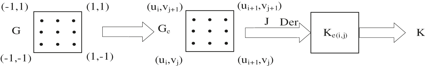
Figure 1: The traditional stiffness matrix solution process

Not all NURBS models are highly continuous, in order not to affect the accuracy of the experiment and increase the universality of the experiment, this paper does not adopt any rule for the time being. The chart of the algorithm in this paper is shown in Fig. 2.

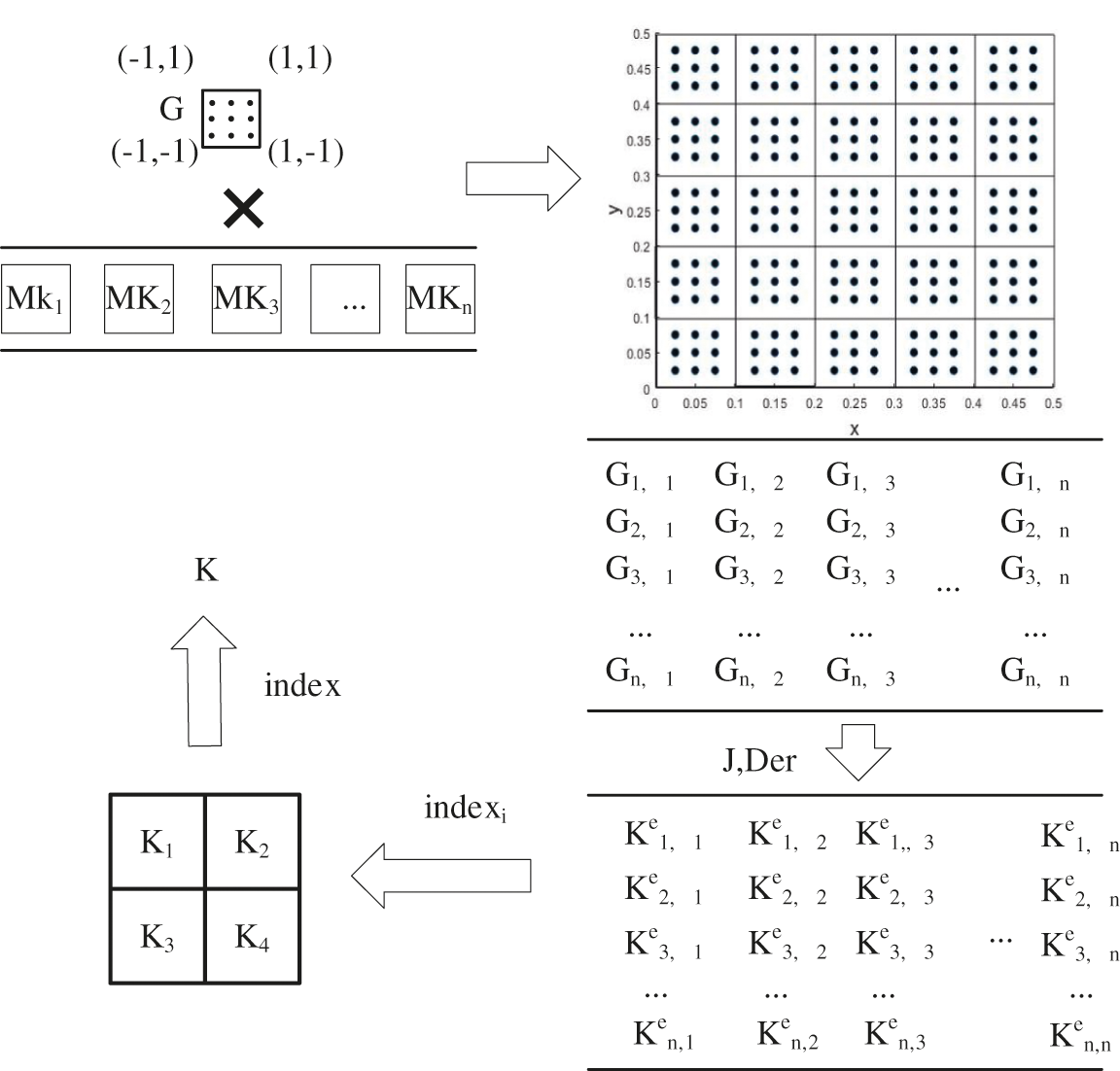
Figure 2: Parallel algorithm flow chart

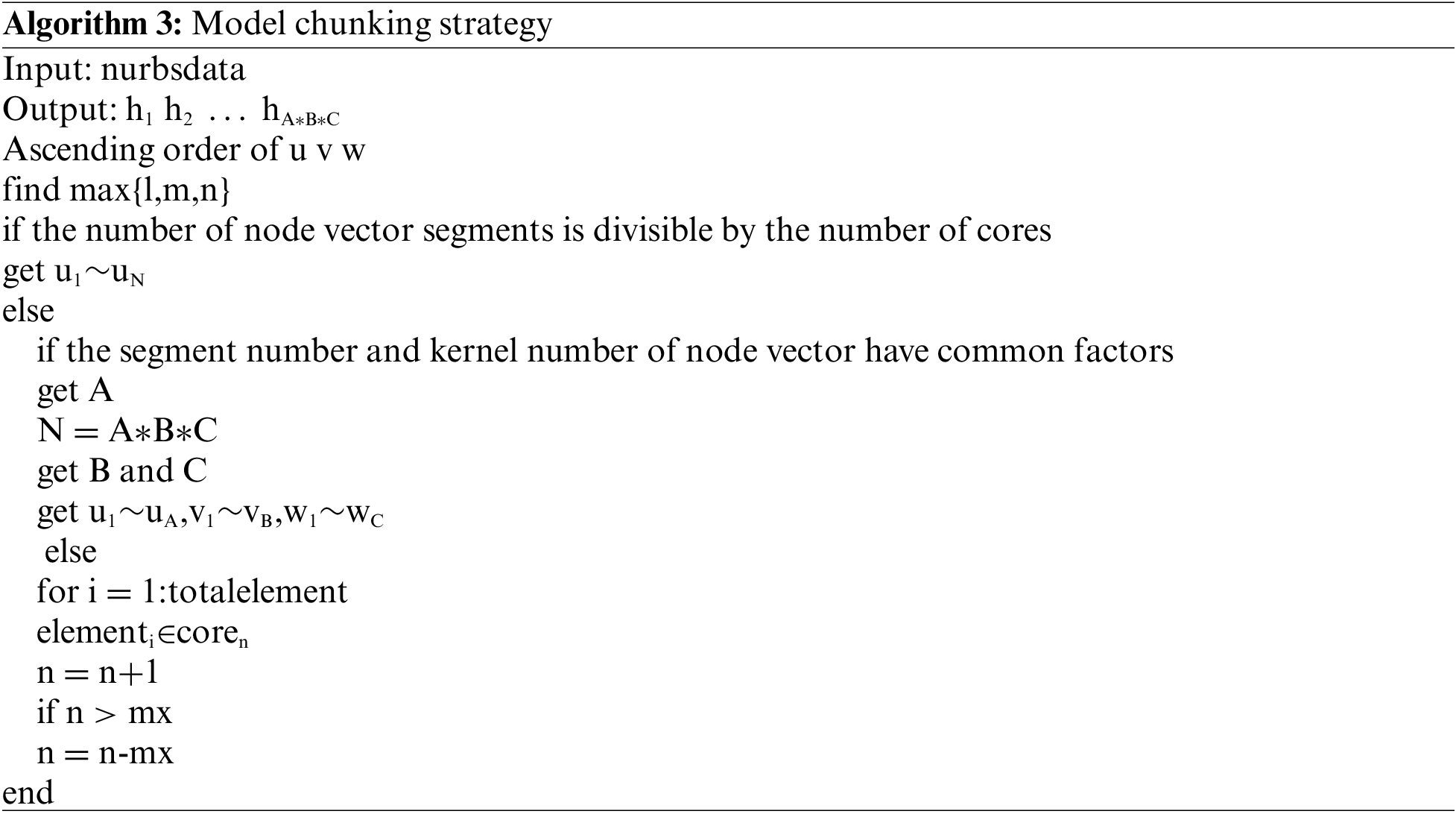
The segmentation proposed in this paper is based on the node vector features and kernel number of each direction of the model. In order to facilitate the subsequent calculation, the amount of computation for each kernel should be roughly the same. The first thing to consider is whether the number of node vector segments (npartu, npartv, and npartw) in each direction can be divisible by the kernel number mx. If it can be divisible, the number of segment segments in each direction is the kernel number mx. If it cannot be divisible, the number of segments is considered to have a common factor with the kernel number, and the kernel number is factorized. The number of segments in each direction is the common factor obtained by factorization. If it is not divisible and has no common factors, the element traversal is carried out in the directions of u, v and w, and each unit traversal is assigned to a core, so as to ensure that the calculation amount of each core is consistent. Each processor’s assigned cell is stored in a cell called gelement.

3.1 Parallel Calculation of the Derivative of Gaussian Integral Points

At first, the number of Gaussian integral points needed to be calculated for each kernel should be allocated. The Gaussian integral points should be divided into mx (Number of cores) regions of roughly the same size based on the number of cores in the computer.

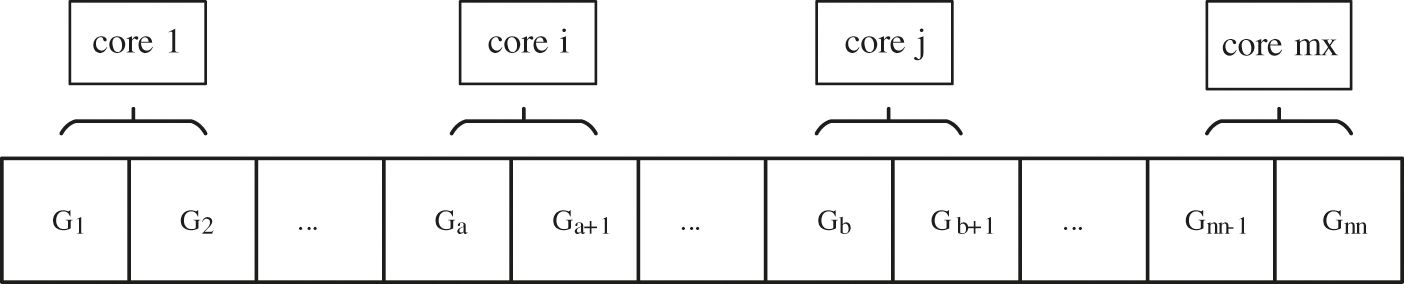
Figure 3: Distribution of computing

According to the properties of NURBS, it is more efficient to calculate the values and derivatives of all non-zero basis functions at a point. It can be found that the calculation process at different points only depends on the interval value of NURBS. Because the interval values of NURBS are fixed, the calculations at different points are independent. Moreover, the number of Gaussian points in each non-zero computation domain is the same, and the computation amount of each Gaussian point is the same. The traditional IGA calculation of Gaussian integral points is carried out in elements, which cannot be carried out in parallel due to the inclusion of many other parameters in element calculation. Therefore, we separate the solution of Gaussian integral points from the calculation steps of element stiffness matrix, so that the calculation can be carried out in parallel.

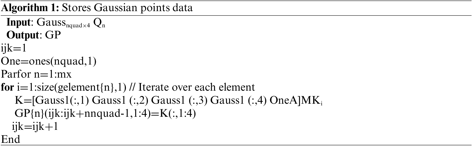
The set of Gaussian points obtained from the above is stored in an element called rule, when calculating the Gaussian integral derivative points need to be in the element coordinates and weight projection to the corresponding physical element domain, then be able to establish a matrix Gaussnquad×3 to store the data and the coordinates of the Gaussian integral points as the result of the Gaussian integral points. Gaussnquad×3 includes two directions of information u, v and the weight W,

Gaussnquad×3=[uvW](16)

The Gaussian integral point can be mapped to an element in the form of matrix. GP can be obtained by multiplying the value of [–1, 1] by the element mapping matrix R, and the weight can be updated and stored in GP. For the below element, its mapping region in the u direction uleni = ui+1-ui, v direction vlenj = vj+1-vj.

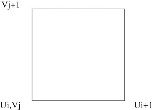
Figure 4: Element area

When the Gaussian integral point is mapped to the whole world, the principle of graphics can be adopted to stretch and translate the low dimension by using the high-dimensional matrix, so the mapping matrix of the original Gaussian integral point is

MKi,j=[(ui+1−ui)/20000(vj+1−vj)/20000(ui+1−ui)∗(vj+1−vj)/40(ui+1+ui)/2(vj+1+vj)/2(wk+1+wk)/21](17)

The same is true for 3D models,

MKi,j,k=[(ui+1−ui)/200000(vj+1−vj)/200000(wk+1−wk)/200000(ui+1−ui)∗(vj+1−vj)∗(wk+1−wk)/80(ui+1+ui)/2(vj+1+vj)/2(wk+1+wk)/201](18)

The information of Gaussian integral points GPn*nquad×4 can be obtained by mapping Gaussian integral points to elements through mapping matrix.

After the corresponding data is stored, Gaussian integral point derivative calculation is carried out. At this time, different processors need to be allocated to calculate the values of Gaussian integral points of different blocks. Assuming that the computer has mx processors, the number of threads is m, and each processor computs a quarter of the total number of nodes, nn/mx. The scale of the derivative of each point in each direction is the product of the order in each direction,

nnel=orderu∗orderv∗orderw(19)

Algorithm 2 is the flow that each processor executes.

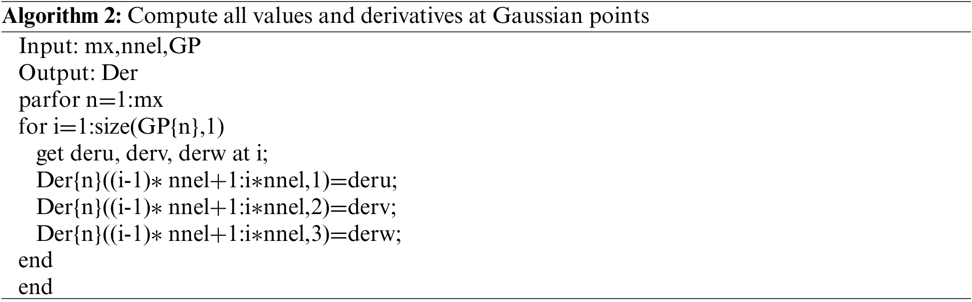
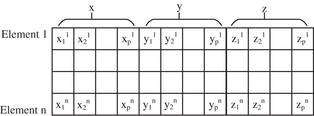
This paper combines the derivative of Gaussian integral points with parallel processing, and uses multi-threads to carry out parallel processing by using the characteristics of multi-core computer. The derivative of Gaussian integral points obtained by each thread is a vector product, the integral is stored as follows:

der=[Der{1}Der{2}⋮Der{mx}](20)

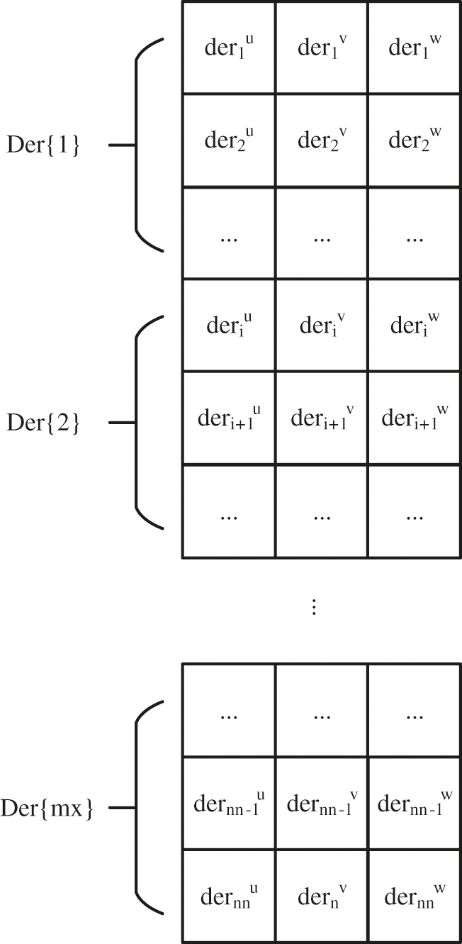
Figure 5: Derivative store

3.2 Parallel of Stiffness Matrix Based on Intermediate Layer

Because model by blocking rules is divided into nuclear number block at first, each processor has stored the relevant elements of the information. Each element can be found in the location of the global and numbered, so local stiffness matrix can be assembled by the loacl index. The global stiffness matrix can also be assembled by the loacl stiffness matrix in this way.

As is shown in Fig. 6, in order to reduce the overlap degree of the boundary of each region after partitioning, we should first consider the order of each node vector. The smaller the order is, the worse the continuity is. In order to facilitate comparison, we can upgrade the three direction node vectors to the same order, and then calculate the number of specific gravity nodes. Then according to the number of segments of the node vector with multiple nodes, the number of segments in each direction is determined. To block the node vector is to find the point where the maximum degree of overlap is located on the node vector. That is to say, the nodes with high degree of overlap can be marked while the order is raised, and then regions can be partitioned according to the marked positions, so as to reduce the border overlap degree of each sub-region after partitioning to the greatest extent.

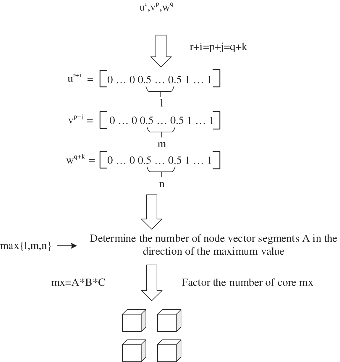
Figure 6: Decomposition strategy when the segment number and kernel number of node vector have common factors

The larger the sub-region is, the closer the individual region is to the whole model; the smaller the sub-region is, the closer the individual region is to a single element. In this paper, the middle layer is adopted for block processing. Simple adjustment in the subsequent application can change the block strategy to make the block region larger or smaller, see in Fig. 7.

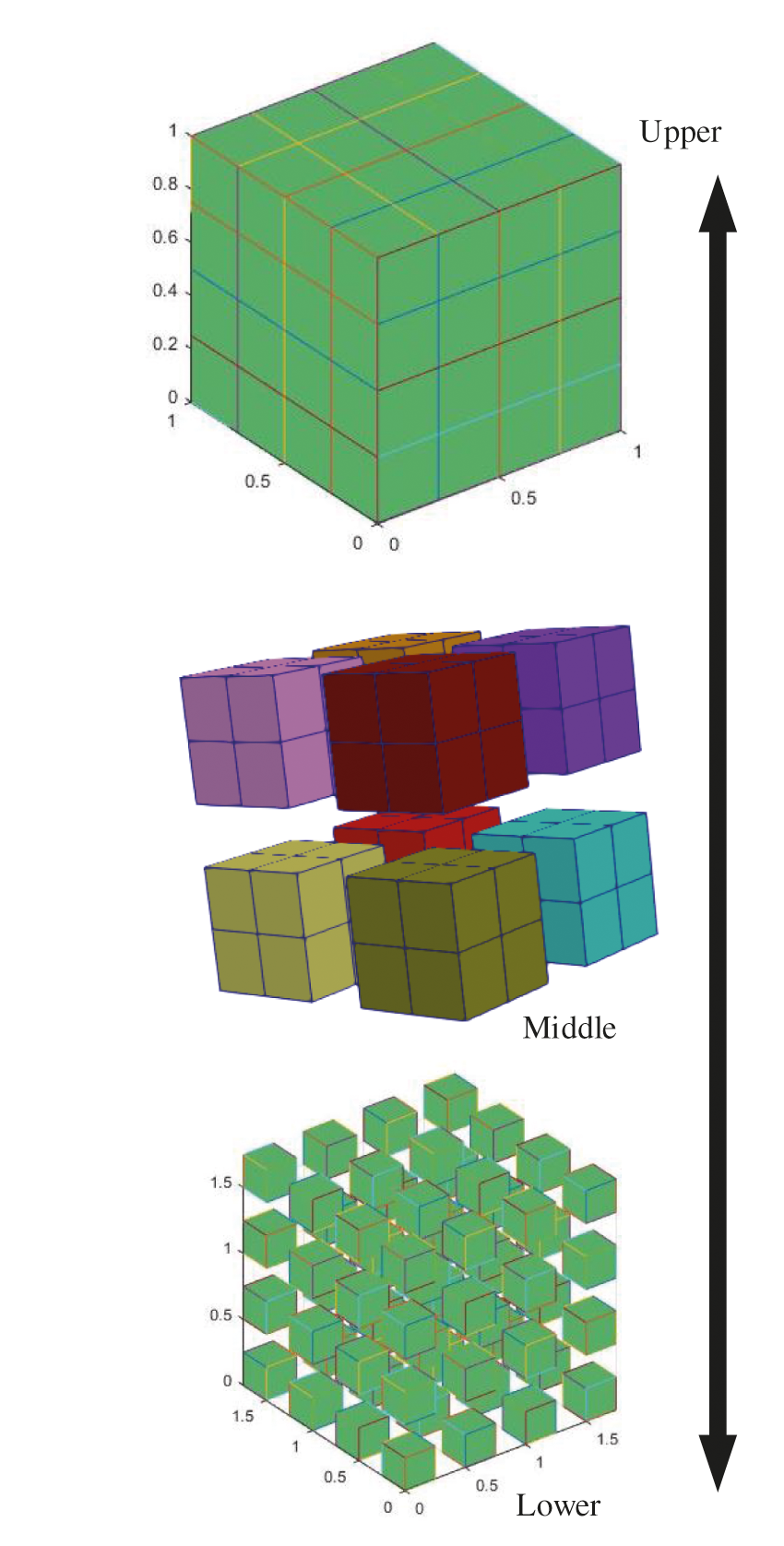
Figure 7: Model block

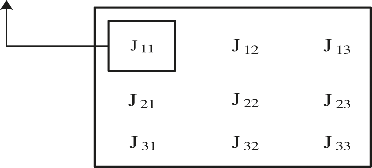
Figure 8: Calculation of jacobian

Since the elements are numbered at the very beginning, a region index can be obtained according to the initial number when calculating regional stiffness, and regional stiffness can be assembled according to the region index, and then the obtained regional stiffness matrix is assembled into the overall stiffness matrix.

When assembling each zone stiffness matrix, the Jacobian matrix is obtained by taking derivatives which greatly increased the workload, making computing time extended.

It can be known from Eq. (7) that the NURBS basis function is obtained by multiplying the derivative of NURBS parameter points with the coordinates of control points

X=F(u,v)=∑i=1ni∑j=1njRij(u,v)Cij

and the Jacobian is

|detDF(ξ,ζ)|=(∂F1/∂u∂F1/∂v∂F2/∂u∂F2/∂v)

>

J111J112…J11n=x11x12⋯x1n∗∂φ1∂u+x21x22⋯x2n∗∂φ2∂u+x31x32⋯x3n∗∂φ3∂u+⋯+xp1xp2⋯xpn∗∂φp∂u

Substituting the Jacobian matrix into Eqs. (2)–(8) through the above equation, the Jacobian matrix can be written in the form of derivative and coordinate multiplication. In this way, the derivation process of the Jacobian matrix is avoided, and the calculation consumption in each traversal element is reduced, so that the calculation time is greatly reduced.

Algorithm 4 is to seek the overall stiffness matrix program.

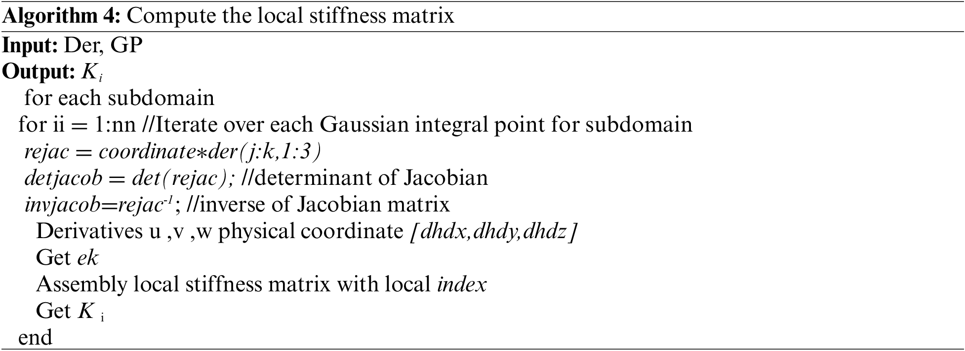
Experiments show that the calculated stiffness matrix may exist bandwidth is larger, the overall stiffness matrix is discrete, calculating is not convenient to follow-up the right item, it will need to get the stiffness matrix of the matrix transformation, the elements, to funnel non-zero element stiffness matrix of the diagonal, enables the calculation to saves time.

Regional stiffness matrix assembly was conducted by regional index, by the middle tier block fixing the control points of each element, determine its position in the regional block, then the element stiffness matrix according to fill in the corresponding position stiffness matrix, finally will regional stiffness matrix through the global index assembly into the whole stiffness matrix.The assembly process is as follows:

K=Kae∗indexa+Kbe∗indexb+⋯Kne∗indexn

4  Analysis of Experimental Results

In this chapter, the algorithm is programed in Matlab2018b, and four different tests are carried out on one PC with i7-6700HQ (4 cores) and 16 GB memory.

4.1 2D Example

It is assumed that the inner wall of the thick-walled cylinder (inner diameter Ri, outer diameter Ro) is subjected to uniform radial pressure P, and the upper and lower bottom surfaces are axially fixed. Due to its symmetry, this paper simplifies the model to 1/4.

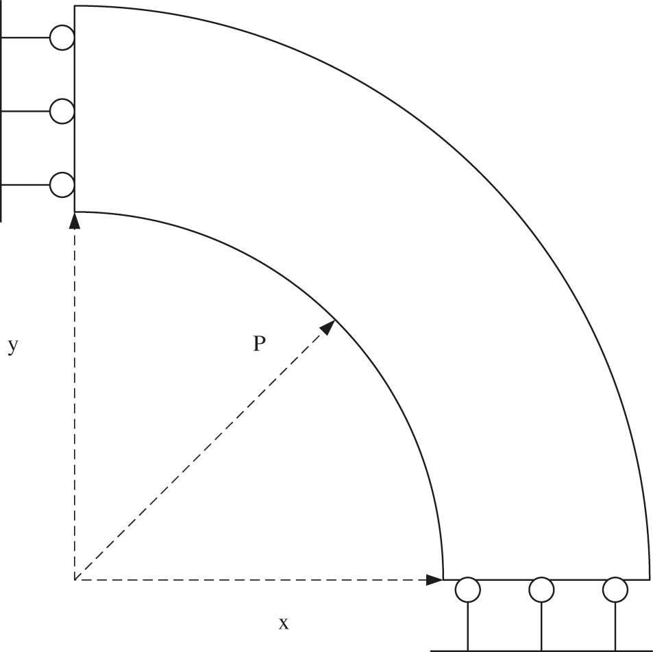
Figure 9: The problem of uniform internal pressure in thick-walled cylinder

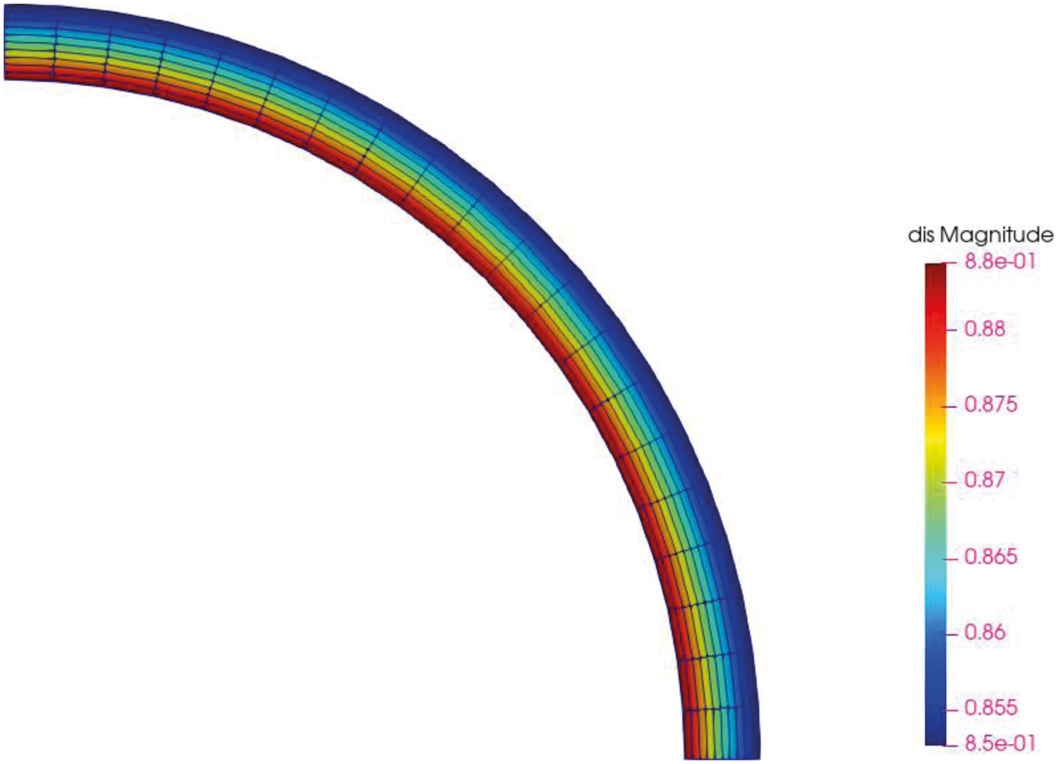
Figure 10: Ring calculation result

In order to compare the results under different degrees of freedom, P subdivision and H subdivision are used to process the original model. In this chapter, only the derivation of the parallel Gaussian integral point and only parallel stiffness matrix assembly are compared with the parallelism of the whole process to show the effect brought by the parallelism of each process. The degree of freedom is controlled by inserting different number of nodes into the original node vector, 21 nodes are inserted initially.

The derivative time of the parallel Gaussian integral point is shown as Table 1.

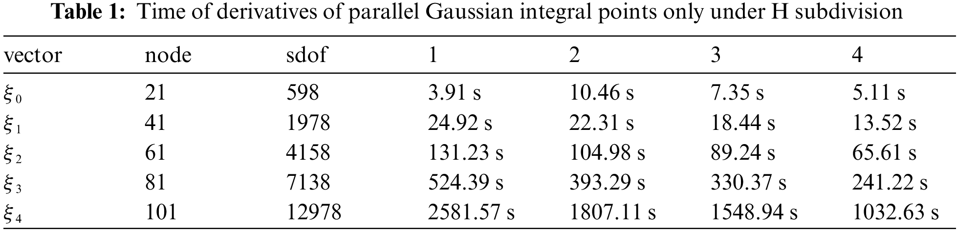
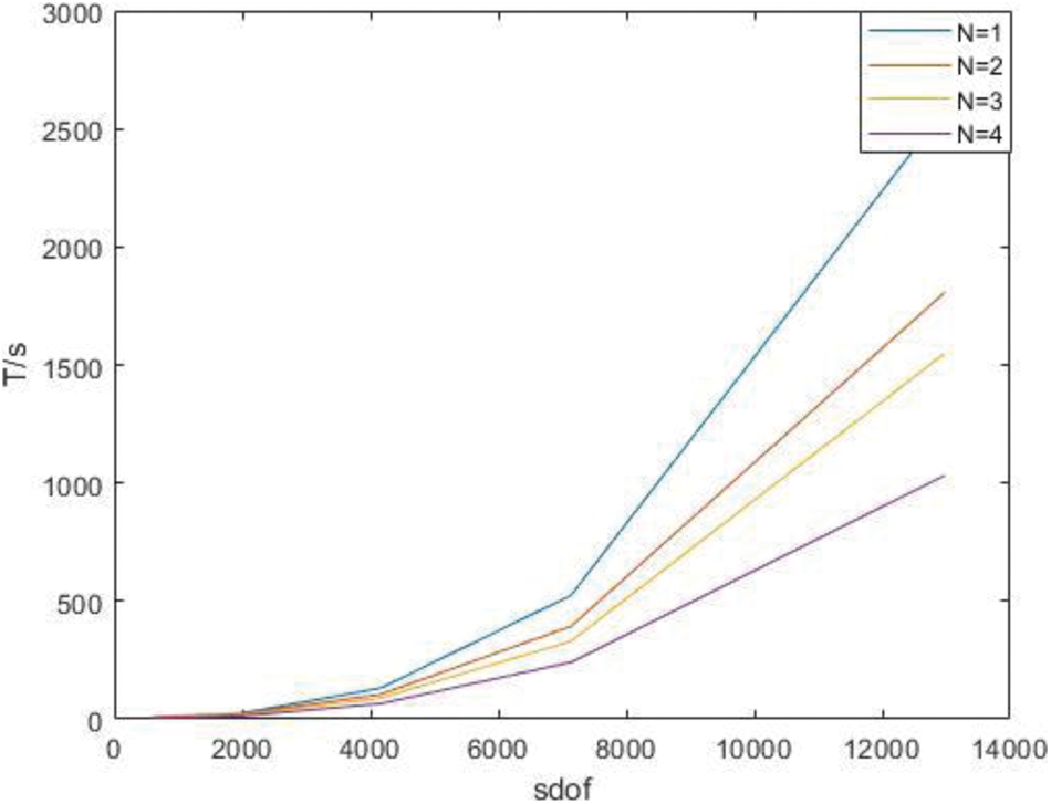
Figure 11: Time of derivatives of parallel Gaussian integral points only under H subdivision

Time of parallel stiffness matrix assembly under H subdivision is shown as Table 2.

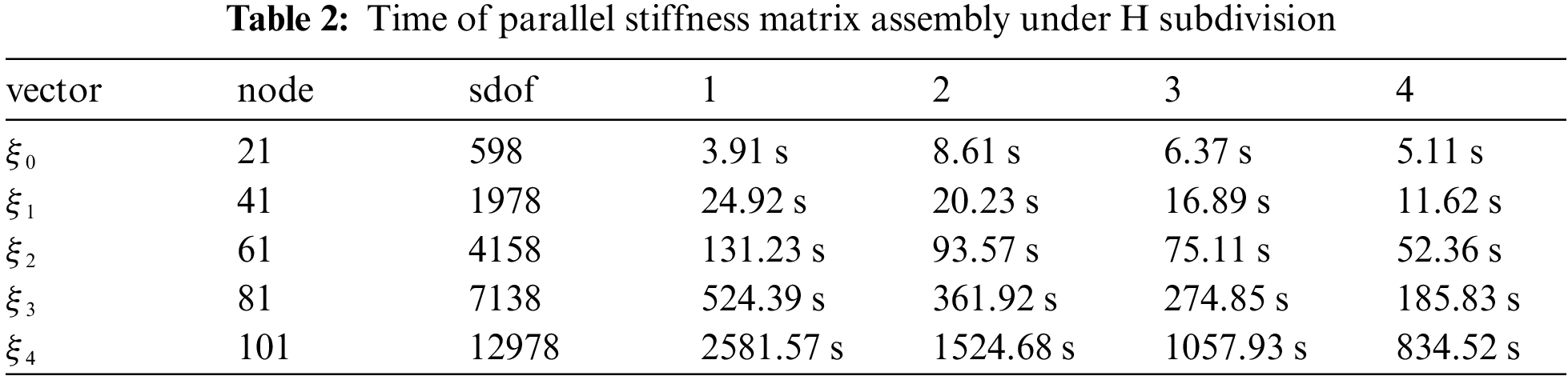
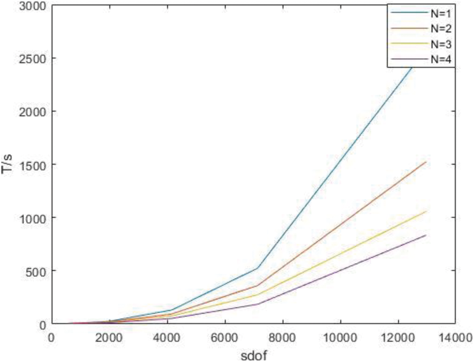
Figure 12: Time of parallel stiffness matrix assembly under H subdivision

Time of the whole process in parallel under H subdivision is shown as Table 3.

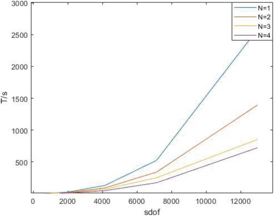
Figure 13: Time of the whole process in parallel under H subdivision

As can be seen from the above chart, the advantages of the parallel algorithm are not obvious when the degree of freedom is low, because it takes time to start the parallel algorithm. With the increase of the degree of freedom, the advantages of the parallel algorithm gradually manifest, and the acceleration ratio tends to the number of processors.

Comparison of the two algorithms under different orders is made by statistics, the number of nodes inserted into the initial node vector is 41, and the order is 3, 2 as shown in Table 4.

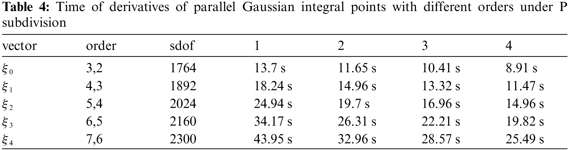
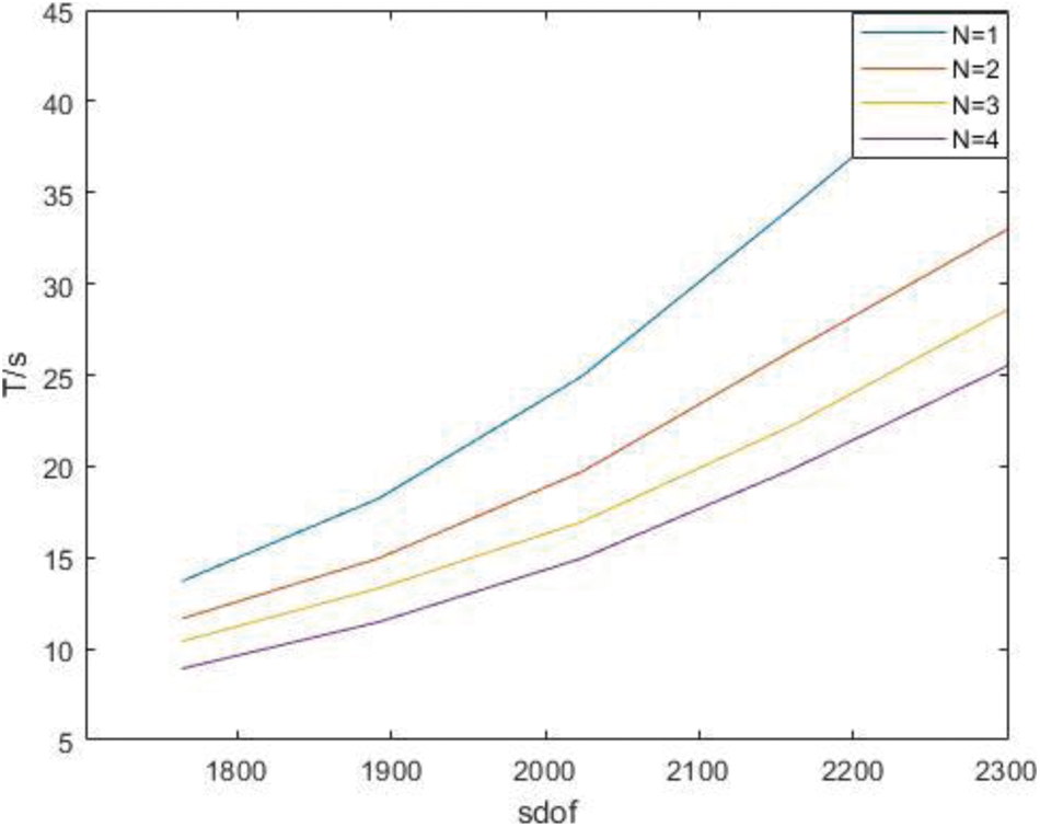
Figure 14: Time of derivatives of parallel Gaussian integral points with different orders under P subdivision

Time of parallel stiffness matrix assembly under P subdivision is shown as Table 5.

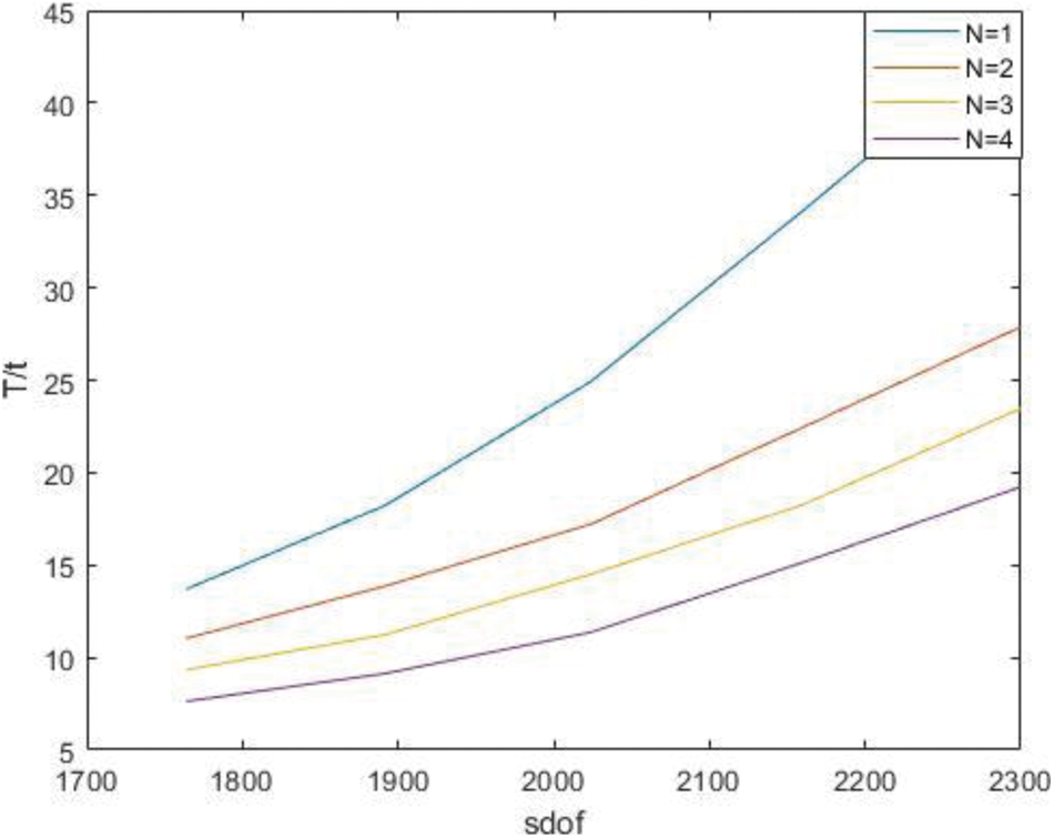
Figure 15: Time of parallel stiffness matrix assembly under P subdivision

Time of the whole process in parallel with different degree under P subdivision is shown as Table 6.

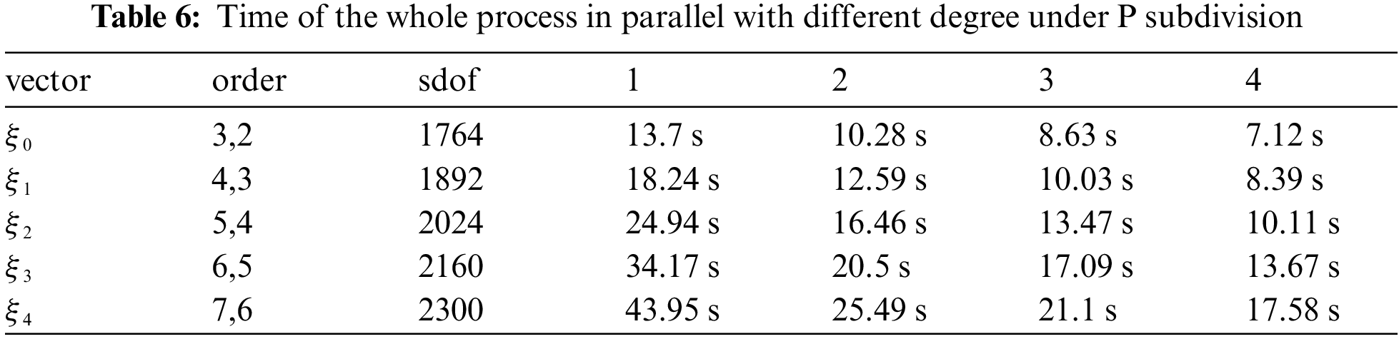
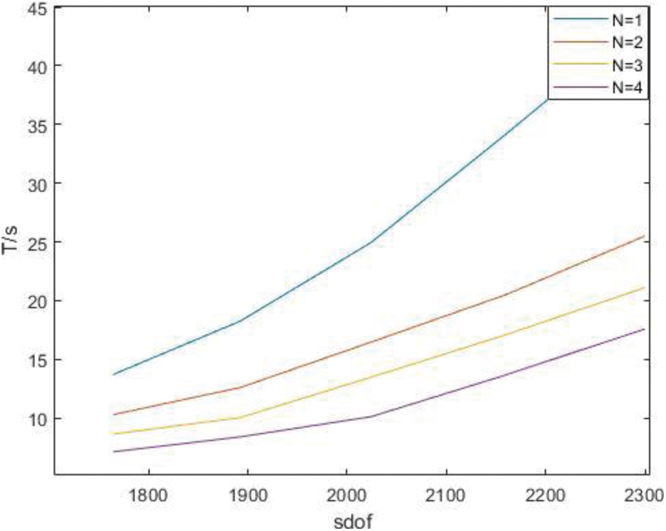
Figure 16: Time of the whole process in parallel with different degree under P subdivision

It can be clearly seen from the figure and table that as the order increases, the degree of freedom increases and the acceleration ratio approaches the kernel number.

After increasing the degree of freedom of the model, the two algorithms were compared, and it was found that whether the number of control points was increased by H subdivision or the order was increased by P subdivision, the parallel algorithm is always less time consuming than the traditional algorithm, the two algorithms are compared. It is found that the parallel algorithm takes less time than the traditional algorithm no matter the number of control points is increased by H subdivision or the order is increased by P subdivision. The calculation efficiency of stiffness matrix can be greatly improved by using multi-thread calculation.

4.2 3D Example

Another example in this paper is the model of the shape of a horseshoe. A load is applied on one side to observe its stress and another side is fixed.

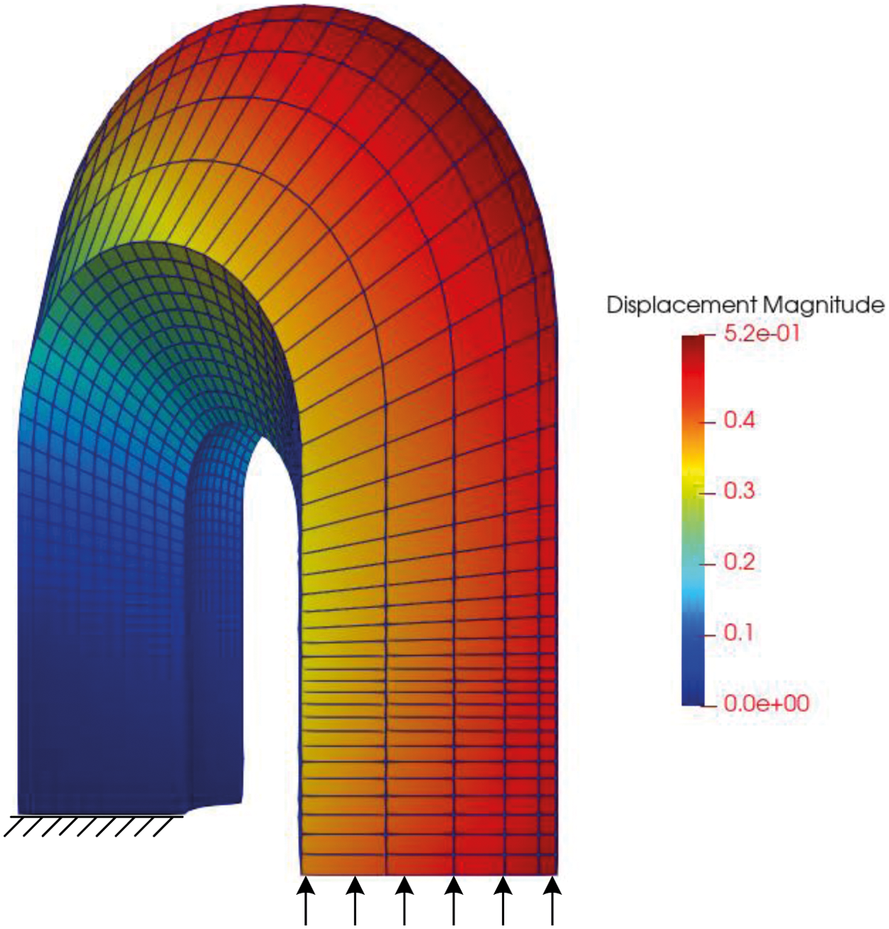
Figure 17: Displacement of horseshoe

The degree of freedom of the model is enhanced by H subdivision. In this example, the dichotomy method is adopted to insert nodes, shown as Table 7.

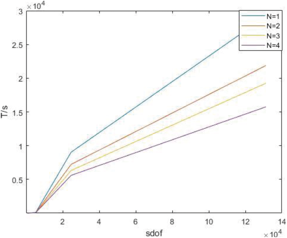
Figure 18: Time of derivatives of parallel Gaussian integral points only under H subdivision

Time of parallel stiffness matrix assembly under H subdivision is shown as Table 8.

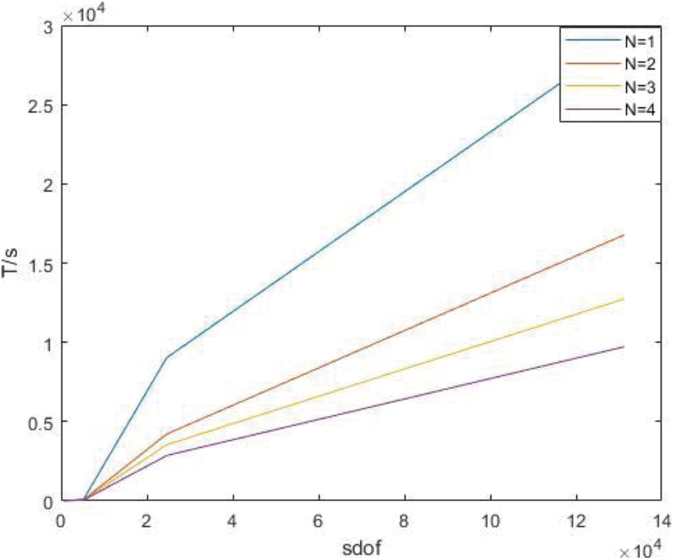
Figure 19: Time of parallel stiffness matrix assembly under H subdivision

Time of the whole process in parallel under H subdivision is shown as Table 9.

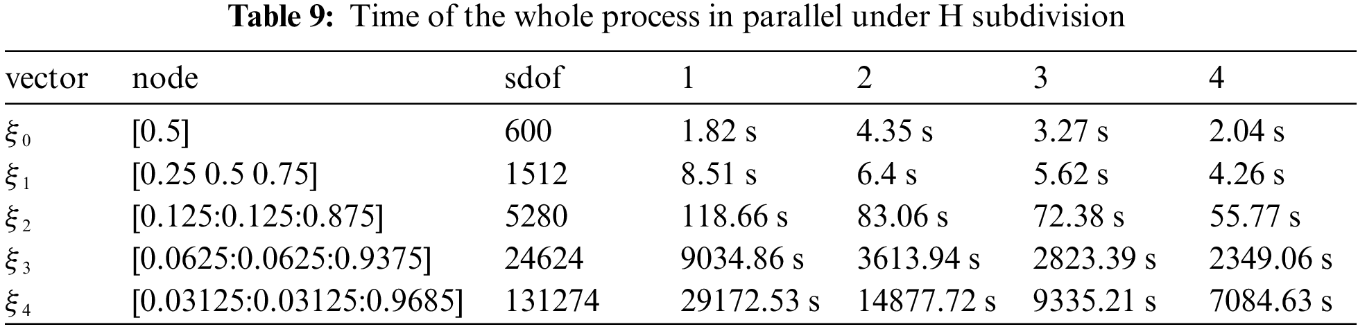
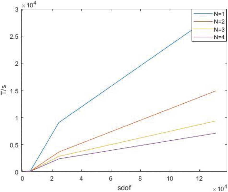
Figure 20: Time of the whole process in parallel under H subdivision

The degree of freedom of the model is enhanced by P subdivision, ξ = [0.125:0.125:0.875], shown as Table 10.

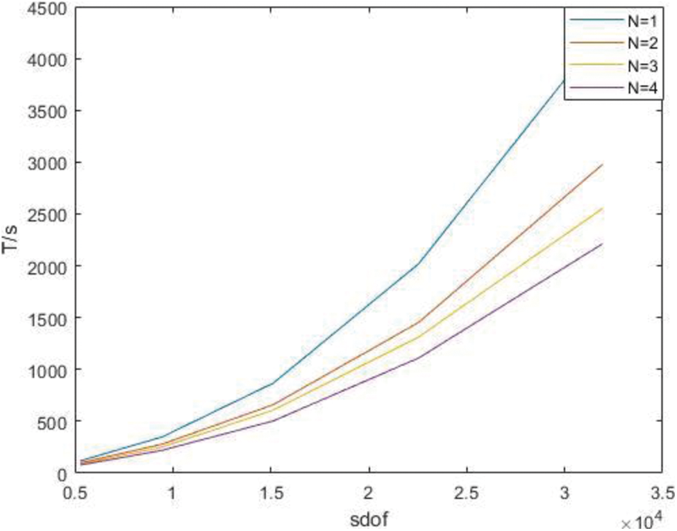
Figure 21: Time of derivatives of parallel Gaussian integral points with different orders under P subdivision

Time of parallel stiffness matrix assembly under P subdivision is shown as Table 11.

Figure 22: Time of parallel stiffness matrix assembly under P subdivision

Time of the whole process in parallel with different degree under P subdivision is shown as Table 12.

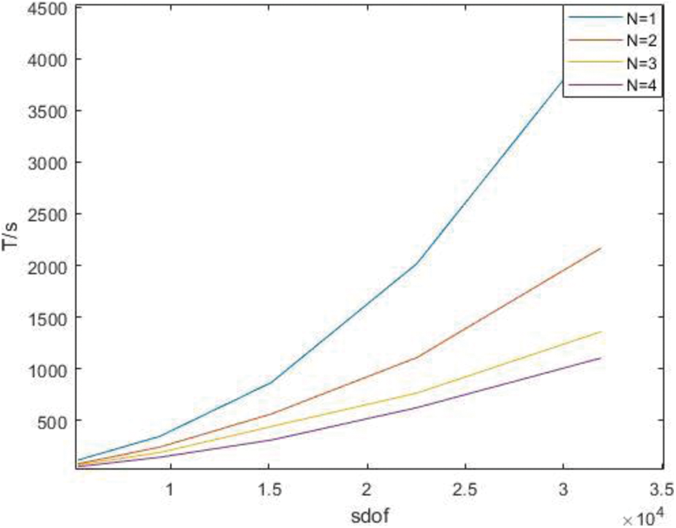
Figure 23: Time of the whole process in parallel with different degree under P subdivision

It can be seen from the above results that with the increase of degrees of freedom, the advantages of the parallel algorithm become more obvious, and when the degrees of freedom are similar, the advantages of the parallel algorithm become greater at high orders. It is found that the stiffness matrix takes up a large proportion of the calculation time in IGA.

5  Conclusion

In this paper, the solution of IGA is accelerated from three aspects. In the first step, the traditional isogeometric solution process is broken, and the Gaussian integral points are mapped to the global model through matrix by using the characteristics of model parameter elements. In the second step, the parallel algorithm PARFOR is used to calculate the derivatives of Gaussian integral points when calculating the derivative of Gaussian integral point, and the derivatives obtained by each kernel are stored in a single matrix. Thirdly, in the assembly process of the matrix, the model is divided into blocks according to the number of the cores and node vectors in each direction, and then different cores are assigned to each region for parallel calculation. Finally, the regional stiffness matrix is assembled by regional index, and the regional stiffness matrix is assembled by global index.

For the future work, it is necessary to focus on the reduction of Gaussian integral points combined with the existing parallel algorithm to further reduce the solution scale in the process of IGA calculation. In the solving process, the stiffness matrix can be divided into blocks and solved in parallel to further improve the solving efficiency.

Funding Statement: This research was supported by the Natural Science Foundation of Hubei Province (CN) (Grant No. 2019CFB693), the Research Foundation of the Education Department of Hubei Province (CN) (Grant No. B2019003) and the open Foundation of the Key Laboratory of Metallurgical Equipment and Control of Education Ministry (CN) (Grant No. 2015B14). The support is gratefully acknowledged.

Conflicts of Interest: The authors declare that they have no conflicts of interest to report regarding the present study.

This work is licensed under a Creative Commons Attribution 4.0 International License, which permits unrestricted use, distribution, and reproduction in any medium, provided the original work is properly cited.