Computer Modeling in Engineering & Sciences

DOI: 10.32604/cmes.2022.019708

ARTICLE

gscaLCA in R: Fitting Fuzzy Clustering Analysis Incorporated with Generalized Structured Component Analysis

Ji Hoon Ryoo1,*, Seohee Park2, Seongeun Kim3 and Heungsun Hwang4

1Department of Education, College of Educational Sciences, Yonsei University, Seoul, 03722, South Korea
2Psychometrics Department, American Board of Internal Medicine, Philadelphia, 19016, USA
3Department of Educational Research Methodology, School of Education, University of North Carolina at Greensboro, Greensboro, 27412, USA
4Department of Psychology, McGill University, Montreal, H3A 0G4, Canada
∗Corresponding Author: Ji Hoon Ryoo. Email: ryoox001@yonsei.ac.kr
Received: 10 October 2021; Accepted: 25 January 2022

1  Introduction

1.1 Motivation

Latent class analysis (LCA) [1,2], as a mixture modeling, has been widely used to identify homogeneous subpopulations from observed categorical variables under the assumption that the population is heterogeneous. One of the reasons for its popularity is its ability to reveal the characteristics of each homogeneous population identified via statistical modeling. Consideration of the heterogeneity also informs the characteristics of subpopulations unveiled in research areas including social, behavioral, and health sciences. Conceptually, identification of unobserved group characteristics via LCA corresponds to unsupervised learning or cluster analysis in data mining such as K-means or K-median algorithm. However, the popularity of LCA as a statistical model is somewhat different from unsupervised learning due to its strict property implemented in the most common estimation method, maximum likelihood estimation based on the expectation-maximization (EM) algorithm [3]. More precisely, the EM algorithm requires multivariate normality for variance-covariance matrix used in the LCA to estimate parameters. As another way of saying, the multivariate normality property prevents researchers from utilizing the concept of big data in LCA, which often produces estimation issues such as non-positive definiteness in computing a Hessian matrix [4].

As described in the comparison between the mixture-modeling approach and cluster analysis procedure such as K-means [5], the mixture-modeling approach does not always perform better than K-means cluster analysis. Rather, Steinley et al. [5] showed an equivalence in terms of statistical modeling under a certain condition. That is, for two conceptually equivalent clustering methods, it cannot be said that the one is superior to the other, which is consistent with the results from Brusco et al. [6] comparing latent class, K-means, and K-median methods. Although Lubke et al. [7] noted that “Model-based methods have the advantage that more rigorous methods can be applied for the comparison of alternative models” (p. 23), it would not be applicable when we consider big data and/or data mining due to the model complexity and strict assumption of multivariate normality. On the other hand, cluster analysis often takes advantage in estimation due to the simple estimation algorithm using an alternative least square estimation in the distance function from centroids. Steinley et al. [5] also noted that “it is important to realize that increased complexity and flexibility do not necessarily imply that a better solution will be found if the goal of the analysis is to uncover the unknown cluster membership.” (p. 76).

Although Steinley et al. [5] highlighted the advantages of K-means, K-means cluster analysis is not a perfect alternative to a mixture-modeling approach. It often suffers from a poor local optimum and has a limitation that its algorithm works with only convex clustering. Such limitation of K-means cluster analysis can be got rid of by applying fuzzy clustering analysis [8]. When fuzzy clustering methods was applied to identification of homogeneous subgroups, the estimation did show less analytic issues such as non-positive definitie matrix. Furthermore, by utilizing the method of how fuzzy clustering analysis can be accompanied by generalized structured component analysis (GSCA; [9]), Ryoo et al. [8] encompassed the LCA in the GSCA framework, which is called fuzzy clusterwise GSCA. In other words, the merger of fuzzy clustering and GSCA allows researchers not only to effectively classify the homogeneous cluster via fuzzy clustering but also to move forward in the model-based classification via GSCA. One of the advantages of LCA over cluster analysis procedures is the capacity to examine the effects of other variables on the LCA parameters, which is no longer the exclusive property of the fuzzy clusterwise GSCA. Such a role of examining the effects of other variables on the LCA was replaced with GSCA in the fuzzy clusterwise GSCA that is a statistical tool of fitting various component-based structural equation models into data [9,10]. In addition, Ryoo et al. [11] provided more indexes that can be utilized in identifying homogeneous subgroups and the procedure of enumerating the number of clusters, which is out of the scope of this manuscript. The method of fuzzy clusterwise GSCA will be described in Section 2.

1.2 Existing Methods and Tools

Although there are many statistical packages including R for latent class analysis and cluster analysis, the method utilizing both the fuzzy clustering analysis and GSCA for LCA is a new approach and thus, there is no comparable R package for fuzzy clusterwise GSCA. Instead, in this section, we introduce three well-known packages for LCA as a mixture-modeling approach: Mplus, poLCA in R, and SAS procedure LCA as competitors. There are many other software packages available but exhaustive search of packages are out of our scope. We focus on their key features of the three packages, which validates the necessity and coverage of our new package, gscaLCA, in R. Note that most statistical programs for LCA include the capabilities of fitting multi-groups LCA, imposing measurement invariance across groups, and implementing latent class regression (LCR). In addition, binary and multinomial logistic regression options for predicting latent class membership and the ability to take into account sampling weights and clusters are also possible.

1.2.1 Mplus

Mplus is the most common software package for fitting structural equation models and provides a variety of tools for modeling. For example, within a mixture modeling framework, both latent class analysis and latent profile analysis are available using the option of TYPE=MIXTURE in Analysis part of Mplus. Latent class analysis is for categorical observed variables, whereas latent profile analysis is used for continuous observed variables. Mplus also provides various estimation methods utilizing the maximum likelihood (ML) method [12] such as MLM (ML parameter estimates with standard errors and a mean-adjusted chi-square test statistic) and MLMV (ML parameter estimates with standard errors and a mean- and variance-adjusted chi-square test statistic). However, Mplus does not provide the stablest and most robust solution of fitting model among statistical software packages in the case of the deviation of data from normality assumption or any other little violation of assumptions such as multicollinearity. Thus, it is often required for researchers to investigate other options to fit in their studies when they are faced with such violations. Nevertheless, Mplus is still versatile in the LCA. Here, listed are a couple of LCA examples using Mplus: van Horn et al. [13] including syntax, and O’Neill et al. [14].

1.2.2 poLCA

Among several R packages fitting LCA, “poLCA” is one of the most common R packages. By using expectation-maximization and Newton-Raphson algorithm, poLCA finds maximum likelihood estimates of the LCA model parameters [15]. Latent class regression (LCR; LCA with covariates) in poLCA estimates how covariates affect latent class membership probabilities. For example, Schreiber [16] used poLCA with a syntax, and Miranda et al. [17] used poLCA to evaluated female young adults’ lifestyle from the behavioral variable measurement in public health, There are two more examples of using poLCA package, van Rijnsoever et al. [18] in information science, and Xia et al. [19] in tourism management. New package, gscaLCA, also deals with the LCR in addition to most of functionalities in the poLCA package.

1.2.3 Proc LCA

Proc LCA was developed for SAS for Windows. Lanza et al. [20] listed key features including multi-groups LCA, measurement invariance across groups, LCR, binary and multinomial logistic regression options. The regression options predicts latent class membership and holds the capability to take into account sampling weights and clusters. Collins et al. [21] described the whole process of fitting LCA including the key features, although most of those key features are also available in other packages, nowadays. Listed are a couple of examples using Proc LCA: Reynolds et al. [22], and Ryoo et al. [23], they explored gifted children’s victimization and bullying by using Proc LCA. As of Jan, 2022, Proc LCA is still requiring additional installation within SAS.

1.2.4 Our Contribution

As mentioned, there is no dominating method to identify heterogeneity of a population between mixture-modeling approach and cluster analysis because each approach has advantages or disadvantages aforementioned and estimation procedures are different. Rather, the choice of statistical model would be related to researcher's discretion [24,25]. Our goal and contribution is to provide an analytic tool for researchers who want to run LCA using a heuristic cluster analysis procedure with fuzzy clustering algorithm and GSCA as a hybrid method. In addition, the utilization of GSCA in gscaLCA allows researchers to analyze data within the full range of the structural equation modeling perspective. We dscribe the package gscaLCA in the four following sections: Framework of fuzzy clusterwise GSCA (FC-GSCA), FC-GSCA with covariates, description of main functions, gscaLCA and gscaLCR, and demonstration of fitting fuzzy clusterwise GSCA with and without covariates by using two empirical examples.

2  Framework of Fuzzy Clusterwise GSCA

Fuzziness is well understood as a soft clustering where each object belongs to every cluster with a certain degree of membership probability, whereas K-means is a hard clustering that every object belongs only one cluster. As a centroid-based clustering approaches, fuzzy clustering overcomes one disadvantage of K-means algorithm in that it does not work well for non-convex data. In addition to the clustering point of view, the fuzzy clustering together with GSCA in estimation process provides tools such as statistical modeling and model evaluation, which is more informative compared with K-means. Model evaluation will be discussed later in this section, which provides cluster validity measures in fuzzy clustering.

2.1 Fuzzy c Means

Based on the description of fuzzy clustering [26] and terminologies [27], we briefly describe fuzzy c means (FCM) algorithm as follows: FCM minimizes the following objective (distance) function, Jm, measured by the sum of squares:

Jm=∑i=1N∑k39=1Kukim‖xi−ck‖2,(1)

where m∈(1,∞] is a classification index, uki indicates the membership probability of ith object in class k, and ck indicates the centroid for class k∈{1,⋯,K}. The m is also known as a fuzzifier, and adjusts the probability of belonging to a class, i.e., m=1 indicates that the membership probability will converge either 0 or 1 such as in K-means, which is excluded in this FCM algorithm. On the other hand, m=∞ indicates that all membership probabilities equal probability in belonging to any of classes, i.e., 1K. Both uki and ck are defined by

ukim=1∑l=1K[‖xi−ck‖2‖xi−cl‖2]1m−1

and

ck=∑i=1Nukimxi∑i=1Nukim.

With a termination criterion such that maxki{|(ukim)(L+1)−(ukim)(L)|}<ϵ for a small value ϵ at L+1 respects, the FCM algorithm is done as follows:

1.  (Step 1) Initialize U(0) for U=[ukim],

2.  (Step 2) Compute ck and ukim by minimizing Jm, which also update U, and

3.  (Step 3) If ‖U(L+1)−U(L)‖≤ϵ then “STOP”. Otherwise, the algorithm repeats from Step 2.

2.2 Generalized Structured Component Analysis (GSCA)

Generalized structured component analysis (GSCA) [9] is a component-based approach of structural equation modeling (SEM). Different from a maximum likelihood-based SEM (ML-SEM), the component-based SEM (CB-SEM) utilizes the underlying construct as a composite of weighted observed variables, and applies an alternating least square method to estimate model parameters. Here, we briefly describe GSCA as a CB-SEM (see Hwang et al. [9] for more detail). The alternating least square method in the component-based approach is relatively simple and straightforward procedure compared to the ML-based approach because it does not assume the multivariate normality of model parameters but minimizes a sum of squares of residuals computed from sample data directly. Along with regularization such as Ridge and Lasso, the least square method produces a more interpretable and predictive model that has possibly lower prediction error [28]. Such a great property of the least square methods is inherited into GSCA [9].

GSCA consists of three sub models: a measurement model describing observed indicators from each latent construct, a structural model defining the associations among latent constructs, and an weighted relation model defining latent constructs. While the typical SEM models include a measurement model and a structural model assuming the normality of the latent constructs [29], GSCA additionally includes the weighted relation model that represents a formative relation between a component and its indicators. That is, the weighted relation model defines each underlying construct as a weighted composite or component of indicators. In this paper, we used both component and latent variable, interchangeably. Such a function in the weighted relation model plays a key role in parameter estimation without a multivariate normality assumption, which eases the estimation. The three sub models of GSCA can be expressed as follows:

Measurement Model:z=ATγ+ϵ(2)

Structural Model:γ=BTγ+ζ(3)

Weighted Relation Model:γ=WTz(4)

where z is a J by 1 vector of observed indicators scores from one observation, γ is P by 1 vector of components, A is a P by J matrix of factor loadings, B is a P by P matrix of structural path coefficients, W is a J by P matrix of weights for components. In addition, ϵ presents the residuals of indicators, which is expressed by a J by 1 vector, and ζ presents the residuals of components, which is expressed by a P by 1 vector. The three equations can be merged into one equation as follows:

VTz=CTWTz+e,(5)

where V=[IWT]T,C=[ATBT]T, and e=[ϵζ].

While minimizing the residual term e in Eq. (5), the factor loadings, path coefficients, and weights are estimated via the alternating least square method. The details of the estimation procedure along with a matlab code can be found in Hwang et al. [9].

2.3 Fuzzy Clusterwise GSCA

As a similar fashion that Hwang et al. [30] applied fuzzy clustering into latent curve model [31], Ryoo et al. [8] applied fuzzy clustering to latent class model. By applying fuzzy clustering to GSCA in the both models, latent curve model and latent class model, the cluster-level heterogeneity can be taken into account. The distinguished feature between Hwang et al. [30] and Ryoo et al. [8] is that the former focused on continuous indicators whereas the latter focused on discrete/categorical indicators. The fuzzy clusterwise GSCA for LCA follows the four steps:

1.  (Step 1) Identify clusters and estimate membership probabilities, ukim, as the initial procedure, where the initial fuzzy clustering works based on the response data.

2.  (Step 2) Estimate the parameters of GSCA model by applying the optimal scaling, si, and the residual sums of squares, ϕ, in Eq. (6).

3.  (Step 3) Update class membership probabilities ukim by utilizing the estimates of GSCA and applying the objective function, Jm, in Eq. (1).

4.  (Step 4) Step 2 and Step 3 are iteratively carried out until both ukim and all GSCA parameters are no longer improved.

In addition to the fuzzy clusterwise GSCA by Hwang et al. [9], the fuzzy clusterwise GSCA for LCA employs the optimal scaling to preserve measurement characteristics of categorical indicators proposed by Young [32] in Step 2. To estimate the parameters of GSCA in Step 2, we minimize the residual sums of their squares weighted with fixed ukim at Step 1 (or Step 3) as below:

ϕ=∑k=1K∑i=1NukimSS(VkTsi−CkTWkTsi),(6)

subject to the probabilistic condition, ∑k=1Kukim=1. si is the optimally scaled vector such as si=f(zi) where f is a optimal scaling function. In Step 3, we update ukim by applying the objective function, Jm, in Eq. (1) for the fuzzy clustering. The fuzzifier, m, of ukim is often set up at 2 in practice [26], which is also used as a default in the R package, gscaLCA. The item response probabilities characterizing classes are estimated based on their membership within each class at the end of procedure. The standard error of estimation can also be calculated by the bootstrap method [33].

2.4 Model Evaluation in Fuzzy Clusterwise GSCA

In addition to R2 type of model evaluation tools, FIT and AFIT, from GSCA [9], the package gscaLCA computes the fuzziness performance index (FPI) and the normalized classification entropy (NCE) recommended by Roubens [34]. They are defined as follows:

FPI=1−K⋅(1N∑i=1N∑k=1Kuki2−1)K−1(7)

and

NCE=−1N∑i=1N∑k=1Kukilog⁡ukilog⁡K.(8)

Both FPI and NCE applies the criterion of “smaller is better” between 0 and 1, which helps researchers decide the number of clusters in the process of fitting LCA [9].

3  Fuzzy Clusterwise GSCA with Covariates

By adding covariates into latent class modeling, we are able to investigate how the covariates predict the latent class membership of individuals [21,35]. Two possible approaches in modeling LCA with covariates can be applied, either a one-step approach or a three-step approach. The one-step approach estimates the effect of covariates on the membership while estimating the class membership probabilities and item response probabilities [36,37]. Specifically, a multinomial regression of membership probabilities on covariates is fitted within the LCA modeling. That is, the combined model estimates all parameters simultaneously. The other approach estimates the effects of covariates by fitting multinomial regressions with partitioning based on the estimated class membership probability. This three-step approach fits LCA at the first step, assigns each subject based on the estimated membership at the second step, and then fits a logistic regression of the assigned membership on covariates at the third step, sequentially [35,38] (see [39] for detailed explanation of three-step approach). Compared to the one-step approach, the three-step approach rarely encounters identification issues or convergence problems because of the separate and individualized steps. Considering these advantages, the package, gscaLCA, applies the three-step approach in the fuzzing clustering GSCA with covariates, denoted as gscaLCR in our package, by examining the covariate effects.

More specifically, the first step of the three-step approach is executing fuzzy clusterwise GSCA, which is explained in the previous section. For the second step, two types of partitioning are available. The partitioning methods are associated with class assignments: either a hard partitioning for mutually exclusive assignment or a soft partitioning based on membership probabilities [35,40]. The hard partitioning assigns each individual's class based on the highest membership probability of the individual. For example, if the estimated uki for the individual i are 0.3, 0.45, 0.25 for class 1, class 2, and class 3, respectively, then the individual is assigned as class 2. On the other hand, the soft partitioning focuses on the membership probabilities themselves for all classes. The estimated membership probabilities are used to assign individuals into each class proportionally. Thus, in the example above, the individual will be assigned class 2 with the probability of 0.45.

With the assignment in the second step, the third step fits either a multinomial or binomial logistic regression. In the case of the hard participating, the procedure is straightforward. A regression model is fitted with the assigned class of each individual as the dependent variable and with covariates as independent variables. The model can be expressed as

log⁡(u¯=ku¯=k0)=β0,k+β1,kcov1,k+⋯+βS,kcovS,k,(9)

where u¯ represents the assigned class with the hard partitioning, k is a focal class and k0 is a reference class. In addition S represents the number of covariates.

For the binomial regression, the assignment is re-coded into dummy variables. By using each dummy variable as dependent variable, the binomial regression can be fitted for each focal class separately. The dummy variables can be denoted as du¯=k for the focal class k, and the binomial regression can be expressed as follows:

logit(du¯=k=1)=β0,k+β1,kcov1,k+⋯+βS,kcovS,k,(10)

where k can be 1,2,…,K, which is the number of classes. The selection of either multinomial or binomial regression is determined by researcher' preference or intention. In the case of soft partitioning, researchers use the same logistic regression as in the hard participating because each participant holds one and only one membership based on the highest probability. However, the regression takes the degrees of their membership into account with weights of the estimated membership probabilities, i.e., soft partitioning. That is, through the weights, the contribution of units on each class within the regression is adjusted.

4  Package gscaLCA for LCA

The package, gscaLCA, enables to conduct a LCA based on fuzzy clusterwise GSCA by estimating the parameters of latent class prevalence and item response probability in LCA with a single command line. The fuzzy clusterwise GSCA model can be fitted with or without covariates. The two main functions of the gscaLCA packages, gscaLCA and gscaLCR, are described below, along with the key features of the results and visualizations it produces.

4.1 Data Input and Sample Datasets

Data are the main input to the function gscaLCA, and they should be formatted as a data frame containing indicator variables and covariates. The function gscaLCA requires the indicator variables to be discrete or categorical. It, however, does not requires whether the categorical variables are integer or character. When any indicator variable is continuous, the function is still run by recognizing the type of variable as a categorical variable. Thus, a caution is necessitated. There is an option that a continuous indicator is assigned as a continuous. On the other hand, for the covariates, both discrete and continuous variable are available. When a covariate is categorical numeric variable, it is required to define this variable as a factor. Missing data should be coded as NA in gscaLCA. The missing values will be deleted for the analysis in the gscaLCA algorithm by applying a listwise deletion in the current version.

The package gscaLCA provides two sample datasets that are informative for exploring different situations: (1) categorical variables (binary and more than two categories) for indicators and (2) continuous or categorical variables for covariates.

4.1.1 TALIS Data

These data provide 5 items from the 2,560 survey responses data of U.S. teachers from the Teaching and Learning International Survey (TALIS) 2018 [39]. Two items are from teacher's motivation, two items were from teaching pedagogy, and the last item is from teacher’s satisfaction. The five items were coded as the ordinal responses from 1 (least) to 3 (most). Teachers’ responses are originally coded as four ordered categorical data. However, due to too small frequencies at the lowest levels at the five variables, we modified them into three ordered categories by merging the two lowest levels: (Not/low importance, moderate importance, and high importance) in motivation, (not at all/to some extent, quite a bit, and a lot) in pedagogy, and (strongly disagree/disagree, agree, and strongly agree) in satisfaction. Other missing codes were treated as a missing code, NA. The specific explanation about the categories and the corresponding question are presented in the manual, which is also accessible via the command of TALIS?

4.1.2 AddHealth Data

AddHealth data consist of 5,144 of the participants including their responses of five item variables about substance use such as: Smoking, Alcohol, Other Types of Illegal Drug (Drug), Marijuana, and Cocaine. The responses of the five variables are dichotomous as either “Yes” or “No” and treated the other missing codes as systematic missings. The AddHealth data additionally includes a randomly generated ID variable and two demographic variables: education level and gender, which can be used as covariates. Educational level consists of eight levels from not graduating high school to beyond master's degree. Gender has two levels, male and female. These data were obtained from the website (https://www.cpc.unc.edu/projects/addhealth/documentation) of the National Longitudinal Study of Adolescent to Adult Health (Add Health) [41]. The study has mainly focused on the investigation of how health factors in young adulthood affect adult outcomes. Although full data collection includes four additional waves since 1994, in the package gscaLCA, only the data of “specific section of substance use” collected at the wave IV are provided, where participants were 24 to 32 years old.

4.2 gscaLCA Command Line and Options

To estimate LCA based on fuzzy clusterwise GSCA with the gscaLCA algorithm, the default function of gscaLCA can be called with the following arguments:

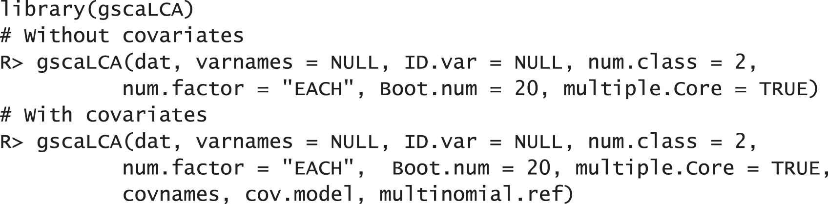
The command gscaLCA requires main seven options to fit the fuzzy clusterwise GSCA that are specified:

•   dat: Dataset to be used to fit a model of gscaLCA.

•   varnames: A character vector. The names of columns to be used in the function gscaLCA.

•   ID.var: A character element. The name of ID variable. If ID variable is not specified, the function gscaLCA will try to search an ID variable in the given data. The ID of observations will be automatically generated as a numeric variable if the dataset does not include any ID variable. The default is NULL.

•   num.class: An integer element. The number of classes to be identified. When num.class is smaller than 2, gscaLCA terminates with an error message. The default is 2.

•   num.factor: Either EACH or ALLin1. EACH specifies the situation that each indicator is assumed to be its phantom latent variable. ALLin1 indicates that all variables are assumed to be explained by a common latent variable. The default is EACH. The specification here presents the relationship between indicators and latent variables, which is used for GSCA algorithm. These two options can be expressed with a diagram, presented in Fig. 1.

•   Boot.num: An integer element. The number of bootstrap to be identified. The standard errors of parameters are computed from the bootstrap within the gscaLCA algorithm. The default is 20.

•   multiple.Core: A logical element. TRUE enables to use multiple cores for the bootstrap. The default is FALSE.

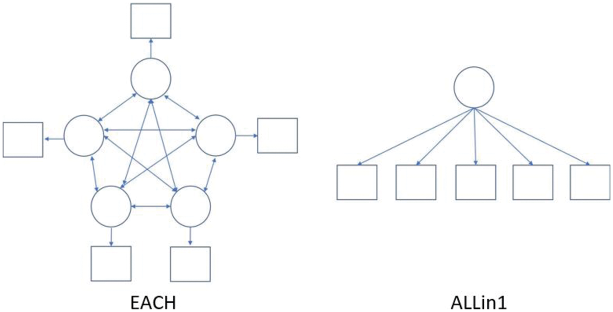
Figure 1: The example of diagrams of the options EACH and ALLin1 with five indicators. The circles represent the latent variables and the square represent indicator variables

When a model of the fuzzy clusterwise GSCA with covariates is fitted, the additional three arguments are required:

•   covnames: A character vector. The names of columns of the dataset that indicate covariates in the model fitted.

•   cov.model: A numeric vector. It is a vector of indicators of whether each covariate is used in specifying three sub-model in GSCA. The indicator is 1 if the covariate is involved in GSCA; and otherwise 0. Involving covariates in the GSCA model indicates that the covariates are used in defining the relation between indicators and latent variables.

•   multinomial.ref: A character element. Options of MAX, MIN, FIRST, and LAST are available for setting a reference group. The default is MAX, which indicates that the class whose prevalence is the highest is used for a reference class in fitting a multinomial regression. Contrary, MIN indicates that the class whose prevalence is the lowest is used for a reference class. FIRST and LAST indicates that the first class and last class are used as the reference class, respectively.

In these arguments, there are kind of generic arguments such as dat, Boot.num, and multiple.Core that utilizes functions in R. On the other hand, ID.var, num.class, num.factor, covnames, cov.model, and multinomial.ref are unique functionalities associated with the gscaLCA package. Thus, a user considers what those values might be and needs to specify them to run gscaLCA.

4.3 gscaLCA Output

The function gscaLCA returns an object involving many different elements. We have selected key features and recommend researchers to check all other arguments by using gscaLCA:

•   N: The number of observations used after applying listwise deletion when missing values exist.

•   N.origin: The number of observations before applying listwise deletion. This number is same as the number of observations of the input dataset.

•   LEVELs: The observed categories for each indicator.

•   all.levels.equal: The indicator whether all indicators used for analysis have the same answer categories. If it is FALSE, the program does not create a graph automatically.

•   num.class: The number of classes used for the analysis.

•   Boot.num: The number of bootstrap assigned by users.

•   Boot.num.im: The number of bootstrap implemented. Not all iterations of bootstrap is needed to estimate the standard error.

•   model.fit: The model fit indices. FIT, AFIT, FPI, and NCE are provided with the standard error and 95% credible interval lower and upper bounds.

•   LCprevalence: The latent class prevalence. The percent of class, the number of observation for each class, standard error, and 95% credible interval lower and upper bounds are provided.

•   RespProb: The item response probabilities for all variables used are reported as elements of a list. Each element consists of a table containing the probabilities with respect to the possible categories of each variable. The standard error and 95% credible interval with lower and upper bounds are also reported.

•   it.in: The number of iteration of in-loop. The in-loop is used for the estimation of the GSCA model.

•   it.out: The number of iteration of out-loop. The out-loop is used to update the membership probabilities of subjects.

•   membership: A data frame of the posterior probability for each subject with the predicted class membership.

•   plot: Graphs of item response probabilities within each category. For example, with two categories, each graph is stored as p1 and p2 in the list of plot. When the number of categories of indicators are different, the graphs are not provided.

•   A.mat: The estimated factor loading matrix of the GSCA model.

•   B.mat: The estimated path coefficient matrix of the GSCA model.

•   W.mat: The estimated weighted relation matrix of the GSCA model.

•   used.dat: The dataset that used for the analysis. When the input data include missing values, the data used are ones after applying listwise deletion.

When the covariates are involved in the analysis, the function gscaLCA returns eight additional elements:

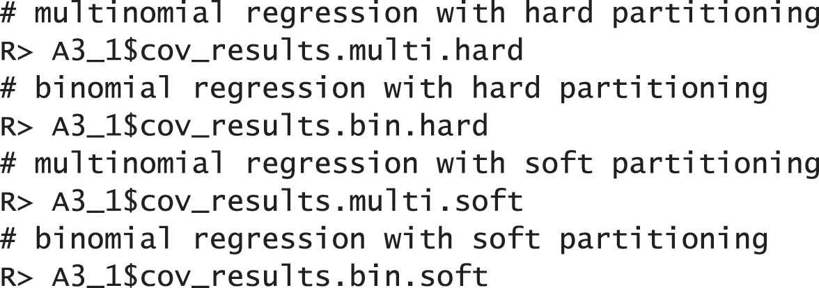
•   cov_results.multi.hard: This is the main result of the multinomial regression with the hard partitioning.

•   cov_results_raw.multi.hard: This is the result of the multinomial regression with the hard partitioning, which is directly from the function nnet::multinom.

•   cov_results.bin.hard: This is the main result of binominal regression with the hard partitioning.

•   cov_results_raw.bin.hard: This is the result of the binominal regression with the hard partitioning, which is directly from the function stats::glm.

•   cov_results.multi.soft: This is the main result of the multinomial regression with the soft partitioning.

•   cov_results_raw.multi.soft: This is the result of the multinomial regression with the soft partitioning, which is directly from the function nnet::multinom.

•   cov_results.bin.soft: This is the main result of binominal regression with the soft partitioning.

•   cov_results_raw.bin.soft: This is the result of the binominal regression with the soft partitioning, which is directly from the function stats::glm.

4.4 gscaLCR Command Line and Options

In addition to the main function gscaLCA, the package gscaLCA provides a function which implements the second and third steps in the algorithm of fuzzy clusterwise GSCA with covariates (gscaLCR). The function is called gscaLCR. As aforementioned, fuzzy clusterwise GSCA with covariate includes three steps. Even if users fit the gscaLCA first without the covariates with the function gscaLCA, steps 2 and 3 of gscaLCR can be executed via the function gscaLCR.

R> gscaLCR(results.obj, covnames, multinomial.ref = "MAX")

The function gscaLCR requires three elements:

•   results.obj: The result object of gscaLCA.

•   covnames: A character vector of covariate names. The covariate variables have to be in the data that used to fit the gscaLCA model.

•   multinomial.ref: A character element. Options of MAX, MIN, FIRST, and LAST are available for setting a reference group. The default is MAX.

The output of gscaLCR is the same as gscaLCA.

5  Example

To demonstrate the usage of the package gscaLCA, we fit two analyses in gscaLCA with empirical exemplars: the one is fitting gscaLCA model without covariate, and the other is the one with covariates. The former is demonstrated with the TALIS data, and the latter is demonstrated with the AddHealth data. It should be noted that although the results of this study were obtained with methodological rigor, they would be slightly different from other researchers’ results within the TALIS study due to lurking variables.

5.1 An Example with gscaLCA without Covariate

For the TALIS data, we used the three-class model (num.class = 3) with a single factor (num.factor = "ALLin1"). It is the optimal model with these data that was found through the model comparison. Regarding the number of class, it is expected to have three factors, motivation, pedagogy, and satisfaction, as the variable name and explanation suggests (see Section 4.1.1). Regarding the number of factors, all variables are supposed to be explained by a common latent variable, because TALIS data is a survey data is collected from U.S. teachers with a topic of teaching and learning. The following command with the function gscaLCA was implemented to fit the fuzzy clusterwise GSCA. Once the gscaLCA command is executed, it displays the degree of the completion process as percentages while gscaLCA is running. When the estimation completes, the summary function is available to display the results. The summary function print out the sample size for the analysis, model fit indices, estimated latent class prevalence, and item response probabilities.

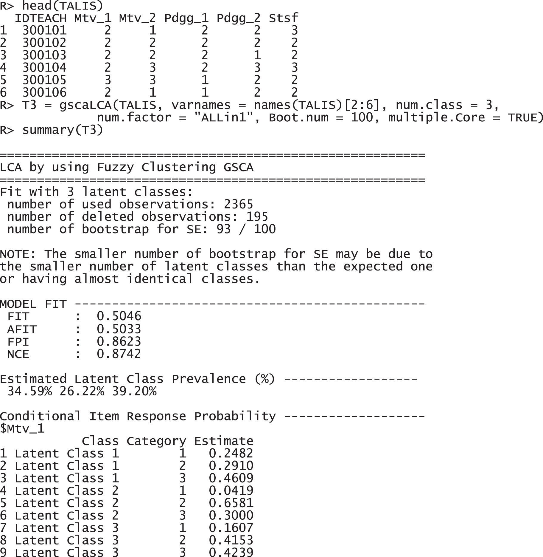
The results report that 2,365 observations were used for the analysis, excluding 195 incomplete responses. FIT and AFIT were 0.5046 and 0.5033, respectively. With a single factor, FIT and AFIT are typically lower than the larger number of factors. The indices to evaluate the classification were relatively large (FPI = 0.8623 and NCE = 0.8742), but they are better than when the option num.factor is EACH for these data. The estimated latent class prevalences is 34.59%, 26.22%, and 39.20%. The conditional item response probabilities for each category per variable are also presented in a table. When the standard error and 95% credible interval of the model fit, the prevalence and conditional response probabilities are required, we can print out the objects through the following commands. These standard error was estimated by the bootstrap.

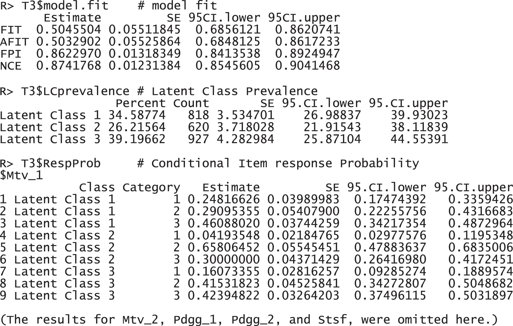
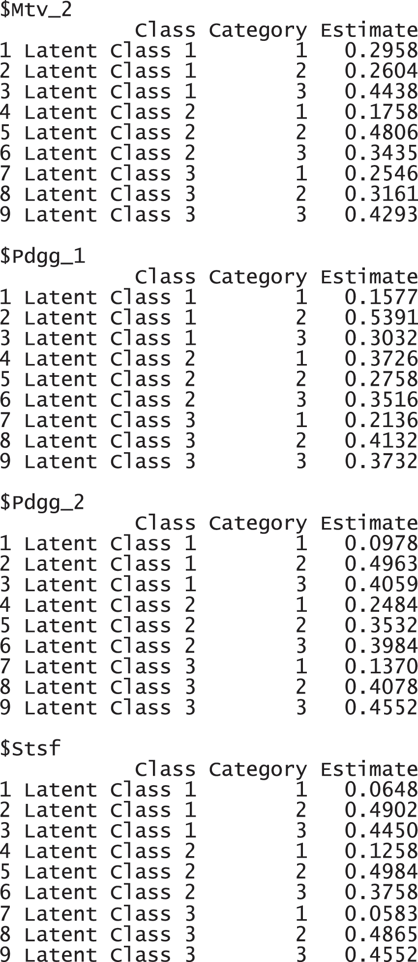
These response probabilities are used to define latent classes. In order to grasp the patterns of the probabilities, a visual representation of profiles based on the probabilities would be more helpful than numeric quantities in the output above. Once the gscaLCA function is executed, the graph is automatically created. When the command summary(T3) is executed, the resulting plot is displayed for all answer categories. When the plots for each answer category are required, it can also be printed by using the command T3$plot. Fig. 2 presents the conditional item response probabilities of the result, T3. Based on the patterns of responses in each class, we define “Pedagogy focused teachers”, “Motivated teachers”, and “Balanced teachers”. For example, for the second response, latent class 1 has relatively higher value in both Pdgg_1, and Pdgg_2 variables, but latent class 1 has relatively smaller value in other variables. Therefore, we define the first latent class as the “Pedagogy focused teachers”. For the second latent class, it has relatively higher value in both Mtv_1, and Mtv_2 variables, but has relatively smaller value in other variables. Therefore, we named the second latent class as the “Motivated teachers”. The third latent class has overall similar values across all five variables, thus, we called the third latent class as the “Balanced teschers”. Lastly, the membership probabilities of observations can be obtained from the membership of the saved objects, T3.

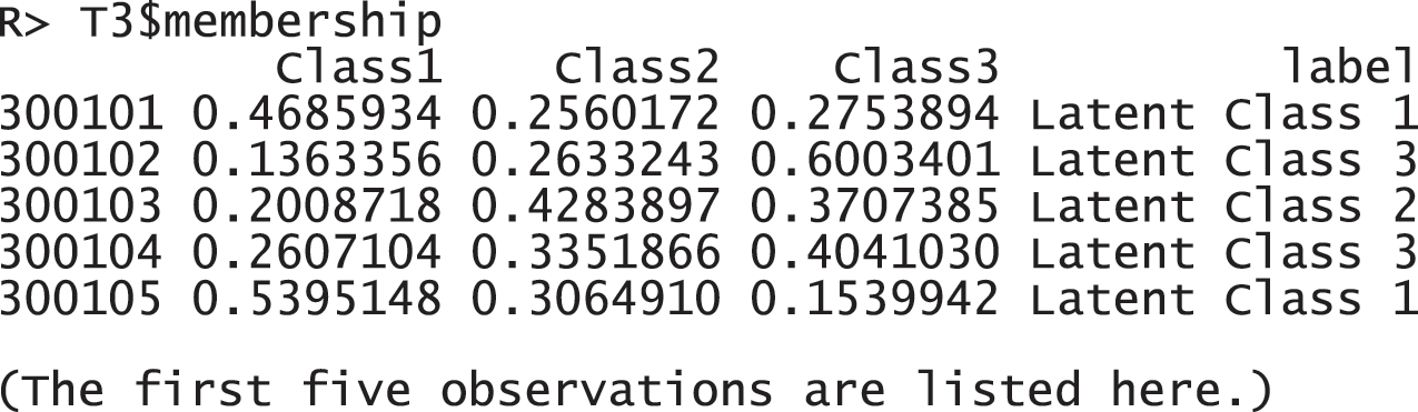
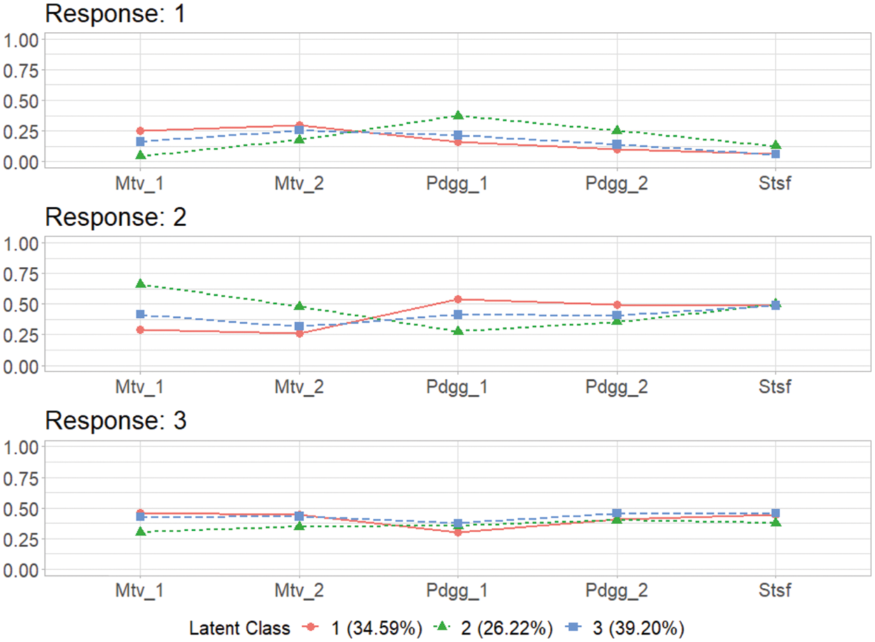
Figure 2: Profiles of three latent classes from fuzzy clusterwise GSCA by using TALIS data

5.2 An Example of gscaLCA with Covariates

In this example, we demonstrate how to fit the gscaLCA with covaritate by using the AddHealth data. We used the three-class model (num.class = 3) with num.factor = “EACH”. which was found in the previous research, Park et al. [10]. For this example, we considered 5 indicators (Smoking, Alcohol, Drug, Marijuana, and Cocaine) and the gender covariate. The gender covariate was involved in fitting the GSCA model (cov.model = 1). Adding the covariate into the GSCA model depends on researchers' decision in their fields, but we recommend to add the covariates into the GSCA model when the covarites affect not only the membership probabilities but also the relationship between indicators and latent variables. When multiple covariates are considered, the indicators of adding the covariates into the GSCA model are presented as a vector. For example, when researcher uses the second covariate out of three covariates in the GSCA model, the option cov.model with c(0, 1, 0) can be used. Fitting gscaLCA with covariates using the function gscaLCA produces the results as follows:

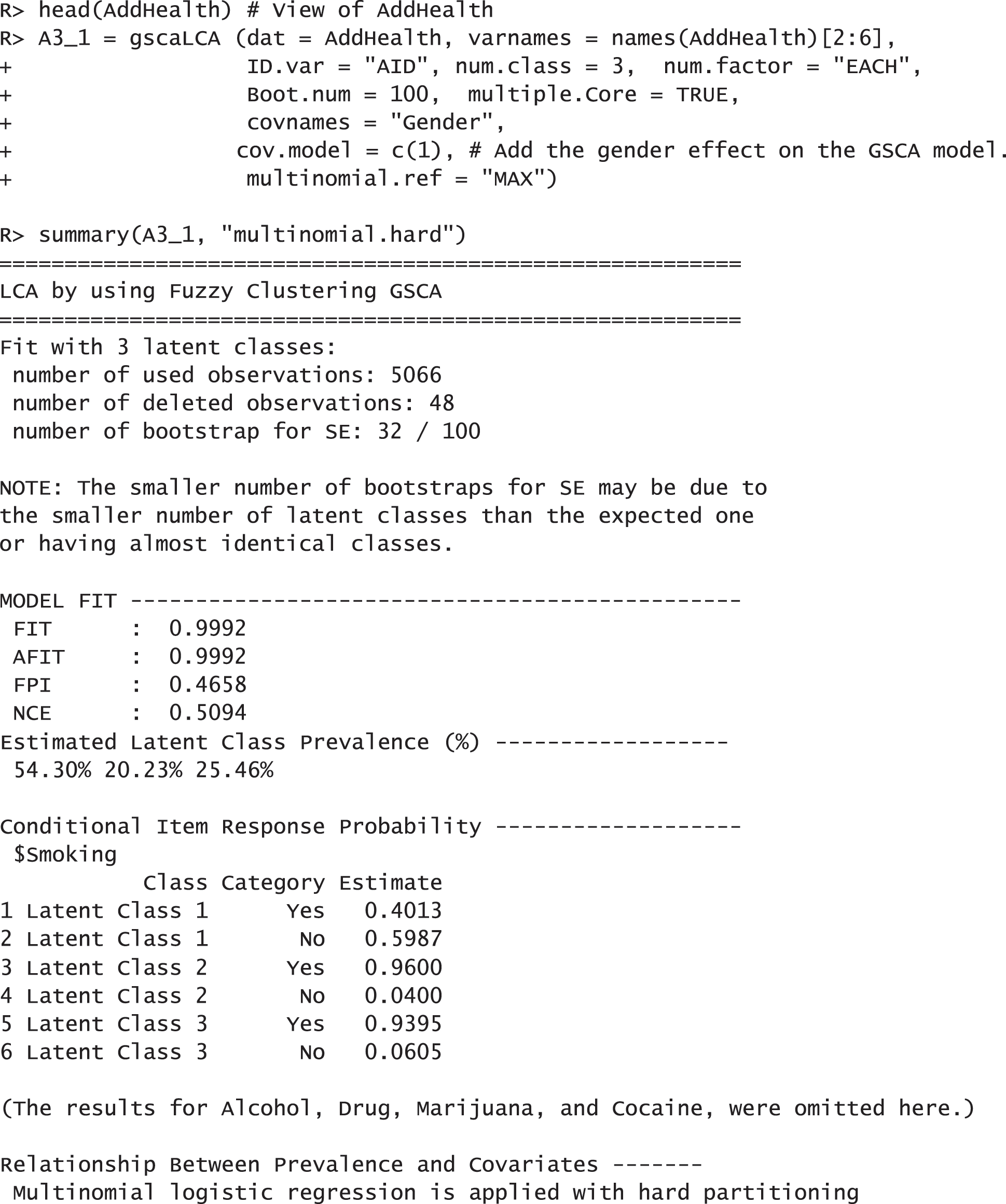
The results report that 5,065 observations were used for the analysis after applying the listwise deletion. They also show that the model fit indices with the AddHealth data are acceptable. FIT and AFIT were 0.9993 and 0.9993, and they are close to 1. The indices to evaluate the classification were relatively low (FPI = 0.4658 and NCE = 0.5094). The estimated latent class prevalences are 54.30%, 20.23%, and 25.46%. These estimated prevalences are changed depending on whether we consider covariates into a GSCA model or not. The conditional item response probabilities are also presented for each category per variable. Like the example of the TALIS data, the results here provide the 95% standard error by using the following commands:

When a category of response is binary, a graph provided by this package shows the probabilities’ patterns of each category. In the AddHealth data, thus the graph is involved when the response is “Yes”, because the responses are binary (Yes or No),

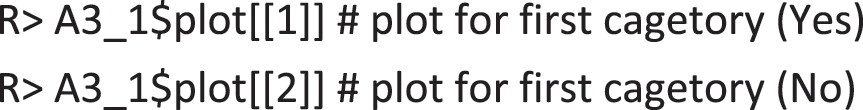
From the plot shown in Fig. 3, three latent class can be defined as “the smoking and drinking class (Latent Class 1)”, “the binge drinking and heavy smoking class (Latent Class 3)”, and “the heavy substance user class (Latent Class 2)” as previously shown in Park et al. [10]. For the case which needs the graphs for all categories of answers, plots for all categories are provided in the results of gscaLCA. Here, the outcome element of A3_1 contains the graphs for each response in plot. The graphs can be extracted by using the following two commands: the one for the category of “Yes” and the other for the category of “No”, respectively.

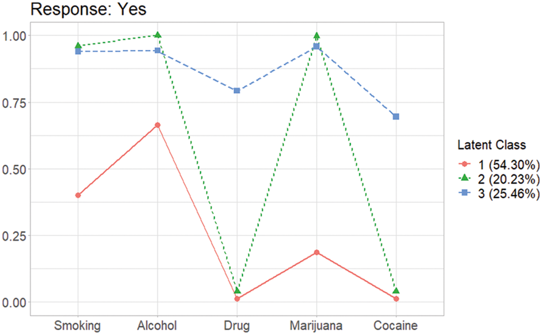
Figure 3: Profiles of three latent classes from fuzzy clusterwise GSCA in AddHealth data when the gender covariate is taken account into the GSCA model

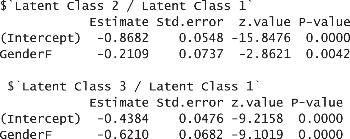
To examine the effects of covariates on the membership probabilities, the function summary can be used as demonstrated before. Other options in partitioning and fitting regression (multinomial.soft, binomial.hard, and binomial.soft) are available as well in the function summary. In addition, the following command also provides the results of regressions:

As the example of A3_1, other options are available for hard and soft partitioning and multinomial and binomial regression.

6  Discussion

Latent class analysis and clustering analysis including fuzzy clustering are statistical tools to identify (dis-)similarity of data distribution as a model-based mixture model and a data-driven classification approach, respectively. We developed the package, gscaLCA, in R that utilizes fuzzy clusterwise GSCA and fit class analysis with covariates as implemented in the other LCA or clustering analysis packages. Moreover, the gscaLCA package allows researchers to consider a structure of underlying constructs by utilizing the GSCA framework. This feature was unique and possible by utilizing least squares estimate. On the other hand, both methods, LCA and clustering analysis, have pros and cons but have been used in various fields at the selection of one of two methods based on researcher's discretion. Based on the theoretical foundation (Ryoo et al. [8]) with its efficiency in estimation, fuzzy clusterwise GSCA is now applicable to latent class analysis within the gscaLCA package, and its extension to latent class regression as a three-step approach is also available.

The gscaLCA package is still undergoing active development until it is equipped with as many mixture models as in the maximum likelihood-based structural equation modeling. Its next journey of gscaLCA is 1) to implement additional options on missing data such as multiple imputation [42], 2) to extend to multiple group and/or multilevel analysis [21], and 3) to extend gscaLCA to longitudinal data so as to fit latent transition analysis [21].

The R package, gscaLCA, provides a unified framework of fitting an LCA model utilizing fuzzy clustering algorithm and generalized structured component analysis. Both dichotomized observed variables and ordered categorical observed variables can be used in the function gscaLCA. In addition, visual representation of results profiles are a key feature in gscaLCA that helps researchers identify characteristics of classes. It should also be noted that the capacities of GSCA [9] within gscaLCA will extend the application of gscaLCA in a variety of SEM modeling.

Funding Statement: This research was supported by the Yonsei University Research Fund of 2021 (2021-22-0060).

Conflicts of Interest: The authors declare that they have no conflicts of interest to report regarding the present study.

This work is licensed under a Creative Commons Attribution 4.0 International License, which permits unrestricted use, distribution, and reproduction in any medium, provided the original work is properly cited.