Computer Modeling in Engineering & Sciences

---

DOI: 10.32604/cmes.2022.020019

ARTICLE

Improved STCA Model for Multi-Lane Using Driving Guidance under CVIS

Xun Li1, Wenzhe Ma1,*, Zhengfan Zhao2, Muhammad Bashir1, Wenjie Wang1 and Xiaohua Wang1

1School of Electronics and Information, Xi'an Polytechnic University, Xi'an, 710048, China
2The Fifth Institute of Electronics, Ministry of Industry and Information Technology, Guangzhou, 440100, China
*Corresponding Author: Wenzhe Ma. Email: mawenzhe0917@sina.com
Received: 29 October 2021; Accepted: 11 February 2022

1  Introduction

The most common traffic infrastructure of urban trunk roads is a two-way road with six or more lanes. The current practice is primarily to broadcast the road condition in real-time, traffic signal, and light timing guidance in order to ensure smooth traffic flow on the road. The inability to improve the efficiency of multi-vehicle road sections using existing means, as well as the forward observation of human driving habits and the influence of the mental state, necessitates the development of Intelligent Transportation Systems (ITS) and 5G, which provide conditions for vehicle and road cooperation to realize the interaction of road condition and vehicle state information [1]. Therefore, under the conditions of future information interaction, it is worthwhile to investigate how to orderly direct vehicle movement and increase traffic safety and road use efficiency [2]. The first problem to be solved is to construct a traffic flow model suitable for characteristic sections under the condition of vehicle-road cooperation [3].

With the development of intelligent transportation systems and intelligent vehicle equipment and the maturing of connected autonomous vehicle (CAV) technology [4], the vehicle operation decision-making process has been able to increase the operation information of surrounding vehicles [5], for example, Tesla's Autopilot System, Volvo's City Safety System, Mercedes-Benz's Pre-Safe System, Honda's Sensing System, etc. [6,7]. Now, large automobile manufacturers have developed intelligent systems for individual vehicles that can provide information about the vehicle's side, rear, and the surrounding environment when the vehicle changes lanes. Intelligent traffic and road infrastructure detection and coordinated control of multi-intersection signal light timing have been enhanced and deployed globally in large and medium-sized cities. Simultaneously, existing navigation software can provide real-time information about road congestion. Therefore, the collected real-time data of vehicle traffic operations from vehicle side and road measurements are used to analyze the influence of interactive information on vehicle lane changing in future traffic environments, which is conducive to providing a theoretical basis for the construction of future traffic infrastructure.

In the future, 5G communications will support vehicle road coordination by implementing intelligent vehicle navigation systems and roadside infrastructure to collect and interact with traffic information [8]. At present, urban traffic video surveillance system in China is gradually developing as the cooperative vehicle infrastructure system (CVIS) [9]. Video monitoring system of urban rail transit cloud synergy technology application architecture design, edge of cloud computing and computing technology was used to construct data perception layer, edge node layer, transport layer, network layer and application layer, business cloud computing center from resource synergy, data coordination, collaborative, intelligent analysis service coordination, coordination, etc., the business application analysis cloud edge of video monitoring system in urban rail transit With the application of technology, speed up the improvement of urban rail transit operation security capability and intelligent level. During the vehicle's operation, the vehicle's running process can use the adjacent driving position, direction, and speed of the vehicle, as well as the driver's intention, as a reference. Obviously, when the traffic information has been got, just waiting for the moment to interact. The major issue that makes the information interactive are: how to make effective use of these data, how an intelligent traffic control model can forecast the next moment for the vehicle, the subsequent position in relation to the vehicle's status, traffic prediction, and the safety of vehicle running security. The degrees of freedom available to a vehicle driver in a lane is limited to acceleration, deceleration, and braking. Effective lane changing can improve traffic flow on the road with an increasing number of lanes, but frequent lane changing increases the risk of vehicle driving. Thus, in order to improve traffic flow while also ensuring vehicle safety, it is necessary to investigate vehicle threats, lane changing rules, and the relationship between the number of lanes. Intelligent lane changing rules in the multi-lane environment can provide useful results, i.e., it can provide intelligent lane change decision-making results for vehicles in multi-lane environment, provide more operation time for drivers, improve safety, and ensure a high density of vehicles of a multi-lane road, and high flow at the same time. Therefore, the research of multi-lane and multi-vehicle lane changing rules is particularly important for the future vehicle road collaborative traffic environment.

At the same time, under the condition of intelligent lane change rules, the impact of the increase of the number of lanes on the increase of traffic flow has not been studied because most of the means of improving the road traffic flow in cities is widening the physical space by increasing lanes. However, the existing studies have discussed the relationship between the number of lanes and the traffic volume. This paper examines the relationship between increasing the number of lanes and increasing traffic flow when the road capacity is heavily mined via intelligent lane changing. The capacity of a multi-lane road is constrained by the collaborative vehicle road environment and human driving habits. The analysis can further reveal the relationship between the two lanes and provide theoretical guidance for the selection of road expansion mode.

2  Related Work

The influence of the collaborative lane change model on microscopic traffic flow is one of the key research directions of intelligent traffic control. The multi-lane SOVM proposed by Lee et al. [10] effectively solves the problem of unpredictable fluctuation of vehicle speed in a large and small area. Lombard et al. [11] proposed a collaborative lane change model based on an online optimization algorithm to vary the parameters of vehicles that adjust their behavior dynamically. Zhou et al. [12] focused on the driver's lane selection and gap acceptance behavior in the classical lane change model, constructed the lane change trajectory model from the driver's perspective and proposed a hyperbolic tangent lane change trajectory model to describe the driver's detailed lane change rules. All of these researches focus on providing driver's lane changing trajectory. Although the model can generate driver-specific lane changing trajectories, the research objective's demand for trajectory-based lane changing is limited.

Li et al. [13] established a lane change cooperative trajectory planning model for connected automated vehicles (CAVS) and solved two key vehicle grouping and motion planning problems. In order to improve traffic efficiency and reduce trip delay and fuel consumption of CAVs in conflict zones, Yao et al. [14] proposed a two-level scheduling and trajectory planning optimization method for CAVs in conflict zones to reduce vehicle delay and fuel consumption. Laarej et al. [15] used energy dissipation and satisfaction to represent the state of vehicles when they were obstructed by other vehicles in driving and studied the vehicle operating characteristics in two-lane mixed traffic flow. Wang et al. [16] proposed a dynamic lane change model of the automatic driving vehicle (AV) considering driver's behavior in a mixed traffic environment, which can effectively complete the lane change action when the mixed traffic system is in cooperative operation and can effectively terminate the lane change behavior when the vehicle is in danger of lane change. Based on the theory of potential energy field, Ma et al. [17] established a lane-changing time model for B-type weaving section of urban road, which quantitatively explained the influence of vehicle spacing on the lateral acceleration of lane changing and deduced the relationship between lateral displacement, longitudinal displacement and time of lane changing vehicles. The deep learning algorithm is gradually mature, and the fusion of sensors and deep learning algorithms can predict vehicle lane changing behavior. Tang et al. [18] proposed a lane change predictor based on an adaptive fuzzy neural network to predict the steering angle of vehicles when changing lanes accurately. With the development of communication equipment, photoelectric sensors are more suitable for information interaction under vehicle-road cooperation. Fakirah et al. [19] proposed a decision-making scheme of automatic vehicle crossing roundabout based on visible light communication (VLC) to coordinate vehicles and infrastructure (V2I), vehicles can pass through a roundabout in parallel. The above research puts forward many lane-changing solutions to the problem of vehicle automatic driving. Then, a traffic planning model is proposed in a simple two-lane environment.

With the increase of urban vehicles and the widening of roads, the problem of multi-lane traffic flow control has gradually become a research hotspot of many scholars. Lu et al. [20] proposed an extrapolation framework based on probability and dynamic traffic load effect to achieve efficient and accurate extrapolation, and studied the probability and dynamic traffic load effect of medium and short span Bridges. Deng et al. [21] divided the lane change conflict strategies adopted by drivers into three categories: conservative, alert and aggressive. Under the condition that the multi-lane change model with random update order of vehicle status and the operation model obtain different space occupancy, different lane change processing strategies will significantly impact the lane change motivation rate and lane change success rate. Hou [22] built a micro traffic simulation model as a research tool, known as NGTSS (New Generation Traffic Simulation System), which is used to analyze the traffic flow characteristics of congestion state in the diversion affected area. The data analysis method of congestion formation and dissipation can solve traffic diversion in multi-lane environments for traffic congestion in urban areas. Tan [23] proposed an optimal control model for the section control layer of the multi-lane expressway that controlled the traffic flow and the maximum average speed. By taking the allocation proportion of each lane as the decision variable, the number of final decision variables is reduced compared with the traditional linear model. Their research objective is to develop a macro method for enhancing road traffic flow. The established method's drawback is that it does not provide clear guidance for micro traffic object vehicle activity in a multi-lane environment and does not analyze the relationship between vehicles. Simultaneously, vehicle position and speed cannot be expressed uniformly in the existing research. Additionally, the model is complex, and the calculation cost increases as the number of multi-targets increases, making it difficult to estimate the memory usage of calculation and communication.

Cellular automata model is a classical model to study micro traffic flow, which can describe the relationship between complex micro traffic objects with a simple model. It can express the basic motion information of position, object velocity, and acceleration in a unified way and has a good ability to model interpretation and description for the complex phenomenon affected by the interaction of a large number of individuals. The characteristics of cellular automata, such as time-space discreteness, state discreteness and action locality, can be consistent with the nonlinearity and discreteness of traffic flow and the complexity of the traffic flow system. The earliest traffic flow model based on cellular automata is Wolfram's “184” model, i.e., the TCA (traffic cellular automata) model [24]. In 1992, Nagel and Schreckenberg jointly proposed NS (Nagel and Schreckenberg) model [25]. The updating rules reflecting the randomness of vehicle motion are added to the “184” model through simple position and speed control rules. For the multi-lane traffic environment, in 1997, Chowdhury et al. [26] proposed the classical STCA (symmetric two-lane cellular automata) model and introduced the two-lane change rule. Following that, Wang et al. improved the model and proposed the STCA-I model in [27]. The STCA-I model attempts to resolve the issue of setting the safety distance in the STCA model and makes the overly cautious and harsh assumption that neighboring vehicles approach at the fastest speed. In order to better simulate the actual high-speed lane changing possibility of vehicles, STCA-I lane changing rules express the interaction between adjacent vehicles and vehicles to be lane changed as risk degree dδ. The STCA-I model maintains a cell gap between the front and rear vehicles as the safe braking distance eliminates the impact of vehicles behind the adjacent lane on the vehicles in the lane following a lane shift. On the basis of retaining a small braking safety distance, it takes the actual speed of the vehicles behind the adjacent lane as the safe lane change condition of the vehicles in the lane change, which improves the flexibility of vehicle lane change on the premise of ensuring safety. Jian et al. [28] proposed STCA-LE model for failed lane changing in unsafe lane changing conditions. In this model, the lateral movement rules of lane changing vehicles are formulated and introduced. However, the rule constructs a lane change model based on the forward visual characteristics of human driving vehicles, and the discussion on lane change safety is not sufficient. Therefore, it is difficult to carry out the comprehensive optimization of single-vehicle dynamic regional information and deal with the existing research and development content of real-time interaction of road vehicle dynamic information [29].

This paper study on safe lane shifting activity focuses on threat assessment under real-time knowledge interaction. STCA-I introduces risk degree to increase the flexibility of safe lane changing and proposes a concept of elastic safe lane changing distance. As dsafe=vmax in the lane change rule of STCA, it is always assumed that the vehicles in the adjacent lane approach at the fastest speed, which makes the safe lane change more flexible. Xu puts forward the X-STCA model [30], which further improves the rule of safe lane changing distance. On the basis of the STCA-I model, Li et al. carried out multi-lane expansion and proposed a multi-lane change strategy based on vehicle road collaborative environment, namely STCA-S model [31]. While maintaining the safety of lane changes, cooperative lane change rules were used to increase the frequency of lane changes and road use performance. Then, for the two-lane setting, the threat evaluation mechanism is constructed using the basic information of position, speed, acceleration, and another interaction, and an improved STCA-M model with guidance under vehicle road cooperation is proposed in [32]. This model, which is based on the improved STCA model, establishes the two-lane vehicle driving guidance function in accordance with the dynamic, safe distance, and real-time congestion state of the road section and guides induced speed and lane change. The STCA-M model is integrated with the induced speed and the threat degree of surrounding vehicles to achieve the role of driving guidance. The explanation of the interaction relationship between vehicles in a multi-lane environment is based on a two-lane road.

This model, based on the improved STCA model, establishes the two-lane vehicle driving guidance function according to the dynamic, safe distance and the real-time congestion state of the road section, and guides induced speed and lane change the explanation of the interaction relationship between vehicles in the multi-lane environment is based on a two-lane road. When applied to a multi-lane setting, it fails to examine the effect of changing multiple objectives and parameters of micro traffic artifacts systematically. Therefore, In previous studies, based on the YOLO v2 model [33], we can extract the characteristics of vehicles, efficiently identify vehicles, and achieve the premise of real-time implementation of lane change rules. Based on the cellular automata model and the improved NS model in [34], this paper proposes a multi-lane change model to accommodate future vehicle road collaborative traffic environments. It analyses the local traffic threat posed by vehicles using simple vehicle interaction data, constructs a driving guidance feature, updates the vehicle's location and speed in response to the driving guidance, and performs multi-lane traffic environment analysis using the STCA-M model. Then, under the condition of vehicle road coordination, a perfect multi-lane change model with lane change guidance is created.

3  Multi-Lane and Driving Guidance Function

3.1 Multi-Lane Model Based on Cell Expression

This paper investigates multi-lane environments that are not subject to external control signals or take the form of converging and diverging roads based on the characteristics of urban multi-lane road environments (for example, three lanes). The purpose is to discuss the relationship between micro traffic objects, i.e., the influence between vehicles and lane changing rules, and analyse the possibility of driving guidance and lane changing rules in mining road traffic capacity. Let consider the cellular automata model from [35]. The target road is divided into three parallel rows of equal-length cells, each representing a cell, as illustrated in Fig. 1. The upper left corner is defined as the vehicle number currently occupying position i, where i represents the lane number and j represents the j-th vehicle in lane i. The lower right corner is the speed of the vehicle in the cell, then the state of each cell at the time it is empty or occupied is shown in Fig. 1.

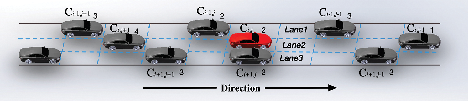
Figure 1: Location and speed diagram of multi-lane vehicles

vi,j(t) and xi,j(t) are used to represent the speed and position of the j-th vehicle in lane i (i.e., in the direction of traffic flow, the number of vehicles decreases) at time t, di,ji−1,j−1(t) is the distance between the front of the vehicle Ci,j(t) and the rear of the vehicle Ci−1,j−1(t) at time t, vmax is the maximum limited speed, the value of velocity is vi∈[0,vmax], the parameter Pdec is introduced to represent the random slowing probability of vehicles. With the time step, the speed distribution of vehicles in each time section is obtained, and the position of vehicles in the next time is deduced according to the speed and the current time position.

3.2 Multi-Lane Model Based on Cell Expression

Due to the interference of front, rear and left/right adjacent vehicles in the process of multi-lane vehicle operation, taking the position of a vehicle Ci,j in Fig. 1 at time t as the reference point, the relationship between multi-lane vehicle and adjacent vehicles at time t is expressed as follows:

1)   Li is the lane i, i = [1, 2,…, n], (i.e., lane number i indicates that there are n lanes on the road);

2)   Ci,j−1,Ci,j+1 represents the front and rear vehicles. In lane i, j, the vehicle Ci,j uses the same corner mark for the corresponding speed and position (vi,j−1(t),xi,j−1(t)),(vi,j+1(t),xi,j+1(t)), respectively.

3)   Cic,j means that the vehicle will change lanes at the next time, and the corresponding pre-lane change position is expressed as xic,j(t), (i.e., the j-th vehicle in lane i at time t will change to lane ic, ic = i ± 1).

4)   When there is a pre lane change vehicle Cic,j at time t, then there is a pre-lane change vehicle for the vehicle, and the front and rear vehicles are expressed as (Cic,j−1), (Cic,j+1), the corresponding position and velocity is expressed as (vic,j−1(t),xic,j−1(t)),(vic,j+1(t),xic,j+1(t)).

5)   The dynamic, safe distance is Dsafei,ji−1,j−1(t).

Let the acceleration at time t be acci,j(t), and the deceleration be deci,j(t). Based on reference [31], this paper deduces and obtains the dynamic safety distance shown in Eq. (1).

if:vi,j−1(t)≤vi,j(t)∀Dsafei,ji−1,j−1(t)=(vi,j−1(t)−vi,j(t))/decmax(1)

Eq. (1) indicates that when the speed of the rear vehicle is greater than that of the front vehicle, the safety distance is related to the speed of the front and rear vehicles and the maximum deceleration.

3.3 Lane Change Guidelines for Threat Assessment

When there is vehicle guidance information, in the process of driving, the vehicle can get rid of the constraints of forward vision, at the same time, it can effectively evaluate the threat of its vehicle in real-time according to the surrounding vehicle information and then carry out the vehicle operation control based on multi-vehicle disturbance. In addition, it can also control the vehicle state according to the vehicle operation state at the far end of the road. Therefore, the multi-lane vehicle lane changing guidance process is divided into lane changing guidance based on local vehicle threat evaluation and lane changing vehicle speed guidance.

In human driving, the proper lane changing process is as follows: obstructed by the front car, judged by the rear-view mirror, and turned on the signal. If we still follow this process under the condition of vehicle road coordination, we will not be able to effectively improve the efficiency of the road to improve the traffic flow situation in local areas. Therefore, we propose a more comprehensive lane changing guidance rule to investigate the status of surrounding vehicles.

According to the parameter description in Section 1, lane changing guidance model is constructed as follows:

1)   Lane change demand. Ci,j is still used as the observation vehicle. In the next iteration step, when the front car blocks Ci,j or Ci,j blocks the rear car, the car needs to change lanes. The judgment affecting the driving of the rear vehicle is added, and improved requirement expression is shown in Eq. (2).

if{vij(t)+xij(t)+dsafe(t)>vij−1(t)+xij−1(t)or vij(t)+xij(t)<vij+1(t)+xij+1(t)+dsafe(t)Li→LicelseLi→Lic(2)

The judgment condition of a lane change in the STCA-I model is just the gap between the front vehicle and the vehicle after a lane change. Obviously, the information of the rear vehicle and forward invisible road condition is ignored, and the global operating environment assessment of local traffic environment is not formed. Therefore, according to the three-lane environment model in Subsection 3.1, the threat assessment function is constructed.

2)   Threat assessment function. Suppose that under the condition of vehicle road coordination, the motion state of surrounding vehicles at t+1 time Ci,j can be calculated, express as Si,j (Situation), then the vehicle space state matrix corresponding to the next iteration step Ci,j can be constructed, as shown in Eq. (3).

Si,j(t+1)=[(vi−1,j+1(t)+xi−1,j+1(t))(vi−1,j(t)+xi−1,j(t))(vi−1,j−1(t)+xi−1,j−1(t))(vi,j+1(t)+xi,j+1(t))(vi,j(t)+xi,j(t))(vi−1,j−1(t)+xi−1,j−1(t))(vi+1,j+1(t)+xi+1,j+1(t))(vi+1,j(t)+xi+1,j(t))(vi+1,j−1(t)+xi+1,j−1(t))]=[Si−1,j+1(t)Si−1,j(t)Si−1,j−1(t)Si,j+1(t)Si,j(t)Si,j−1(t)Si+1,j+1(t)Si+1,j(t)Si+1,j−1(t)](3)

The Ti,j(t+1) of threat degree evaluation for a vehicle Ci,j at t+1 time is expressed as follows:

Ti,j(t+1)=Si,j(t)[−Si−1,j+1(t)Si−1,j(t)Si−1,j−1(t)−Si,j+1(t)Si,j(t)Si,j−1(t)−Si+1,j+1(t)Si+1,j(t)Si+1,j−1(t)]−dsafe(t)(4)

The elements of the threat evaluation function are traversed to obtain the location of the minimum value Liguide=min(Ti,j),i=1,2,…,n;j=1,2,…,m−1 which represents the lane change guidance of vehicle Ci,j at t+1, where m is the maximum number of vehicles in the cooperative control environment. From Eqs. (3) and (4), when the lane number i = {1, 2, … n}, the corresponding Si−1,j±1(t)=NanorSn+1,j±1(t)=Nan.

3.4 Speed Guidance Based on Lane Change

The multi-lane expansion is carried out according to the NS-S model developed in [34], and the vehicle speed at time t is compared to the front, and rear vehicles, after which the induced speed of the vehicle i is increased to vi,jguide(t), which involves lane change guidance, and the acceleration acci is the same as the NS-S model. The induced speed is calculated using the NS-S single-lane model when there is no lane transition. If a lane shift occurs, the induced speed is calculated based on various road conditions.

1)   Induced vehicle speed based on forward vehicle movement trend after a lane change

In the current road conditions where the vehicle road cooperation technology has not yet been realized, the motion state of the front vehicle depends on the driver's experience judgment, and it will cause a certain acceleration delay, which provides room to improve the efficient use of the road. Based on the interactive hypothesis of vehicle speed information, this paper proposed Eq. (5) for observing the induced speed of a vehicle Ci,j under the condition that the movement trend of the front vehicle is known.

vic,jguide−f(t+1)=min{(vic,j(t)+acci,j),(vic,j−1(t+1)+acci),vmax}(5)

The vehicle's speed (guide-f, front) is related to the acceleration trend of the vehicle in front following lane change to achieve the effect of synchronous acceleration.

2)   Induced vehicle speed based on backward vehicle movement trend

Under the condition of obtaining the vehicle interaction information, the vehicle can take the active acceleration rule-following lane change to ensure the synchronization movement and avoid the rear-end accident. After lane change, the induced speed should meet Eq. (6) under the condition of obtaining the backward vehicle running trend,

vic,jguide−b(t+1)=min{(vic,j(t)+acci,j),(vic,j+1(t+1)+acci),vmax}(6)

Under the condition of vehicle road coordination, it can also be associated with the acceleration trend of the rear vehicle (guide-b, back).

3)   Induced vehicle speed based on near blocking point

When the traffic density is higher than the critical value, the road blocking point is inevitable. Even under the condition of free flow density, the blocking point may still produce (ghost phenomenon) and propagate backward, resulting in the stop and go state of vehicles. If we can give early speed guidance to the vehicles going to the blocking point, then the linear deceleration and acceleration process will improve the smoothness of the road, the fuel economy, and environmental protection of the vehicles. Therefore, we add the speed regulation rule based on the near blocking point under vehicle road coordination.

Referring to the method of searching the blocking point in reference [36]. If the condition of Eq. (7) is satisfied and the number of blocked vehicles m≥3, then it is determined that there is a blocking point, and the last vehicle in the blocking point is set as the reference position xi,jamj(t) of the blocking point.

di,ji,j−1(t)=di,j−1i,j−2(t)=…=di,j−m+1i,j−m(t)=0∩vi,j⁡(t)=vi,j−1(t)=…=vi,j−m(t)(7)

where m count the number of vehicles contained in the blocking point. The first car's starting speed at the blocking point is determined using the idea of a slow start that corresponds to the actual situation. In a cell distance, the dissipation time of the blocking point is tjam=m−1 simulation steps, and the induced speed value for subsequent vehicles that do not reach the blocking point is all calculated using Eq. (8).

vi,jguide−j(t+1)=min(vi,j(t),mod(di,ji,jam(t)/tjam)(8)

To sum up, there are seven induced speeds according to the lane change demand. The Ci,j can determine the location of the blocking point and the lane where the speed limit is located. According to the optimal speed selection principle of safety priority, the induced speed at time t Ci,j is obtained, as shown in Eq. (9).

vi,jguide(t+1)=min{vi,jguide−f(t+1),vic,jguide−f(t+1),vi,jguide−b(t+1),vic,jguide−b(t+1),vi,jguide−j(t+1),vic,jguide−j(t+1),vmax}(9)

3.5 STCA-L Model

Under the condition of vehicle-road coordination, through Eqs. (2)–(9), the change of vehicle speed is correlated with the speed of the preceding and following vehicles on the current road and adjacent roads and the congestion of the road ahead. The goal is to reduce stop-and-go traffic on roads. The state of parked vehicles improves the synchronization phase in the road section. The guided update rules of STCA-L model are shown in Eqs. (10)–(14):

1)   Lane changing rules based on threat assessment:

Li,j(t)→Lic,j(t),|Ti,j(t)|>Dsafei,ji−1,j−1(t)(10)

2)   Acceleration rule based on induced speed:

vi,j(t+1)=min(vi,jguide(t),(vi,j(t)+acci),vmax)(11)

3)   Deceleration rule based on near blocking point:

vi,j(t+1)=min(vi,jguide−j(t),vi,j(t),Dsafei,ji−1,j−1(t))(12)

4)   Random slowing down:

vi,j(t+1)={max(vi,jguide(t+1),vi,j(t)+accmax),randi(t)<pcmax(vi,j(t+1)−deci,vi,j(t)+accmax),randi(t)≥pc(13)

In Eq. (13), pc is the probability of complying with the induced speed; randi,j(t) is the random number generated by vehicle Ci,j in the random slowing iterative step, and the value is [0,1].

5)   Location update:

xi,j(t+1)=xi,j(t)+vi,j(t+1)(14)

4  Numerical Simulation and Analysis

This section presents the numerical simulation and analysis of the basic vehicle motion information that may include the interaction speed, acceleration, and local congestion point information in the assumed CVIS (Cooperative Vehicle-Infrastructure Systems) condition. The vehicle model is mainly classified into two types as type I and type II. The type I vehicle is any vehicle that has at most 7 seats, while the type II vehicle is any vehicle that has at least 8 seats. In this paper, we only consider the type I vehicle in our numerical simulation and analysis. According to the actual vehicle motion characteristics, the simulation data is initialized as follows: The shape of the vehicle, length and width are: Clength≤5m,Cwidth≤2m; acceleration of acceleration: 0.4g≤aadd≤0.8g,g=9.8m/s; acceleration of deceleration:−1.2g≤adec≤−0.8g,g=9.8m/s; Meanwhile, it is assumed that the frequency of information exchange is 1 Hz. According to the dynamic safety distance function proposed in this paper, the cell represents the road length of 5 m (i.e., cell=5m). Within the updating frequency time of vehicle acceleration and deceleration speed information, the range of position change i: Position range of acceleration process: 2m≤xi(t+1)−xi(t)≤4m; Position range of deceleration process:4m≤xi(t+1)−xi(t)≤5m. Under extreme acceleration conditions, the corresponding position change of the vehicle is less than or equal to one cell. Vehicle density is calculated as ρ=m/L, where m is the number of vehicles on the road with a simulated lane length of L.

In the simulation road, the lane length is L = 2 km, consisting of 400 cells with the number of lanes n = [2, 3, 4, 5]. The maximum speed is based on the speed limit of urban roads with more than 3 lanes in Xi'an, China, as shown in Fig. 2. Select vmax = 4 cells/s = 72 km/h; The simulation time is 10,000 steps, and the initial speed is randomly distributed in the road according to 0−vmax. To reduce the influence of the initial distribution, the statistical range of the simulation results is within the range of 5000–10,000 steps.

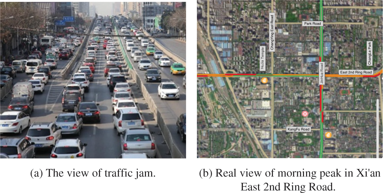
Figure 2: Real view of urban multi-lane

4.1 Speed and Flow

The paper reproduces STCA, STCA-I, STCA-S, and STCA-M, respectively. Numerical simulation of STCA-L, in which the curves corresponding to STCA and STCA-I are multi-lane extensions to its two-lane model. Lane speed curves (i.e., 2, 3, 4, and 5) are obtained as shown in Figs. 3a–3d. The flow curve is shown in Figs. 4a–4d. The fundamental indicators such as average speed and average flow are compared under different vehicle densities in the numerical simulation results in each sub-figure.

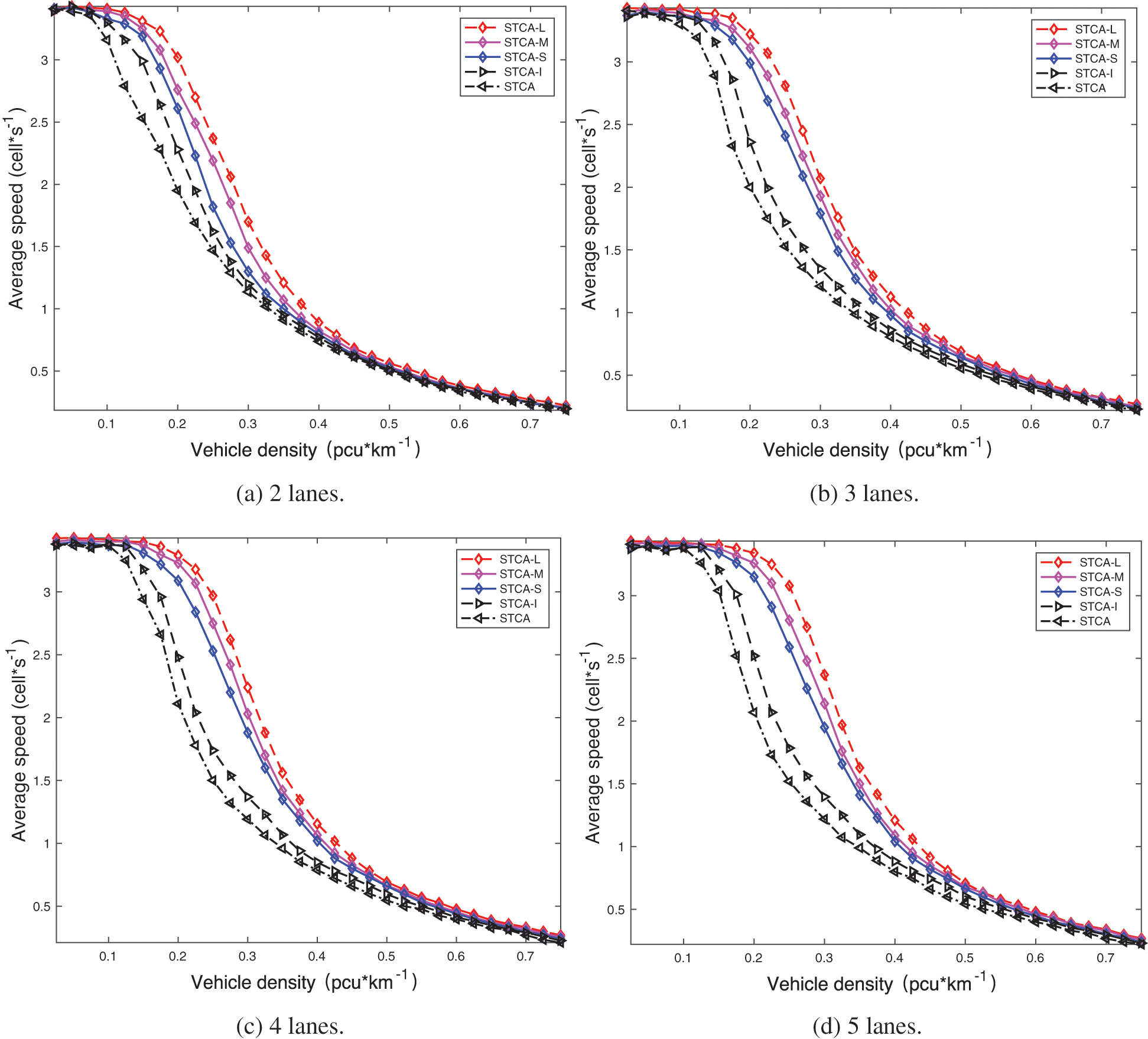
Figure 3: Basic diagram of the multi-lane average speed curve

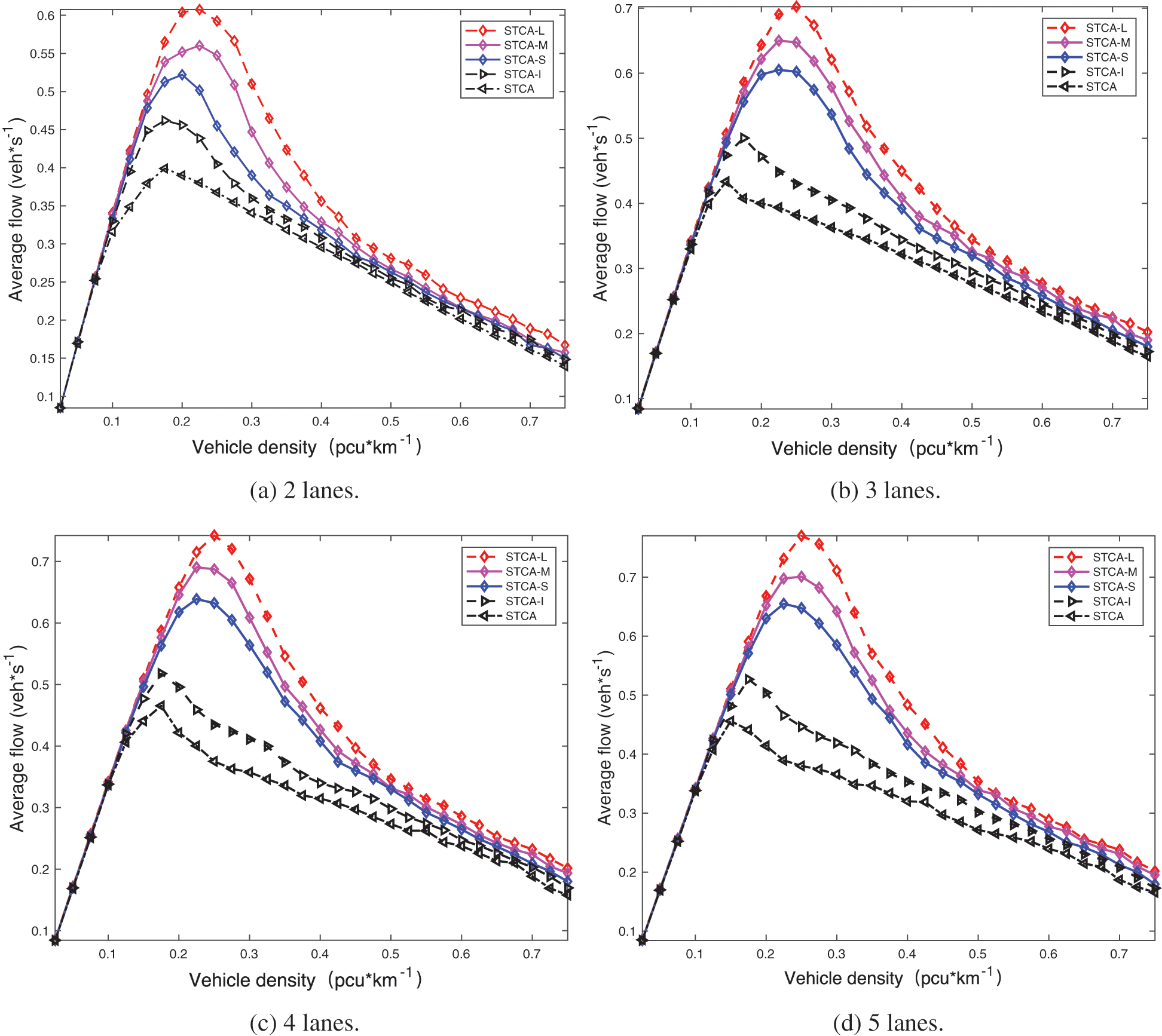
Figure 4: Basic diagram of the multi-lane flow curve

Analyzing the average speed data curve in Fig. 3 shows that: The extremely low vehicle traffic density, i.e., the value is about [0, 0.075] pcu/km. Road resources are abundant, vehicles are in the free-running stage, and vehicles do not need to change lanes to maintain speed or have sufficient, safe lane change intervals. Therefore, the vehicle speeds of the microscopic objects under the 5 models are the same. When the vehicle density further increases, tending to 0.1 pcu/km. The STCA model requires more stringent lane-changing requirements and a fixed safety distance setting, causing vehicles to slow down and wait for lane-changing, so the average speed first drops significantly. At the same time, careful observation can find the vehicle density range [0.1, 0.325] pcu/km, the average speed of the 4 models has the same changing trend, but corresponding to the same vehicle density, the STCA-L model can obtain a higher average speed value. This is because on the basis of ensuring safe lane change, STCA-I is more flexible than STCA, STCA-S is more flexible than STCA-I, STCA-M is more flexible than STCA-S. The proposed model (STCA-L) in this paper provides the most flexible lane-changing rules for the multi-lane environment. Enable the vehicle to pass through possible lane changes and maintain the vehicle's speed. From Figs. 3a and 3b, we observe that when the two-lane is expanded to the three-lane, the average speed of the STCA and STCA-I models has a large gap with STCA-S, STCA-M, and STCA-L in the vehicle density range [0.15, 0.35] pcu/km. This shows that the three-lane STCA-S, STCA-M, and STCA-L models have considered both forward and backward vehicles simultaneously. This collaborative control method based on global considerations can provide more lane-changing possibilities. When the vehicle density exceeds 0.4 pcu/km, the average speed value corresponding to different models, STCA-L cannot obtain speed maintenance, which shows that the average flow of the road section is effective but limited by the coordinated control method. The increase in the absolute number of vehicles will cause the control method to fail.

In Fig. 4, as the average vehicle speed changes within the vehicle density range [0, 0.1] pcu/km, the average flow of the five-lanes model is the same due to the similarity of the absolute number of vehicles (i.e., the lane can be changed smoothly without changing lanes or without guidance and deceleration under free-flow conditions). However, with the further increase of vehicle density, the demand for lane changing has increased significantly. Whether the lane can be effectively changed has a direct impact on the average flow value. The flow increases with the increase of vehicle density by changing lanes, but different lane changing rules give the road different flow characteristics: when the vehicle density rises to 0.175 pcu/km, the STCA model average flow reaches its maximum. The STCA-I model provides more lane changes to enable maximum traffic flow than the STCA model. Although the STCA-S model can further increase the average flow through more flexible lane changing rules, there is still an inflection point when the vehicle density is 0.2 pcu/km. The STCA-L model explores the possibility of changing lanes and maintains the vehicle speed at a relatively high vehicle density, thereby obtaining a better average flow. Compared with the other four-lane model, the STCA-L model can reach the maximum flow when the vehicle density is 0.25 pcu/km. By observing Fig. 4, we could find that the vehicle density range from [0.15, 0.275] pcu/km, through effective lane change, the vehicle speed can be maintained in a more extensive density range, and the vehicle speed of road sections, especially high-speed vehicles, can improve the higher use efficiency of the road section. In order to more accurately characterize the differences between the models, the specific data are compared, as shown in Tables 1 and 2.

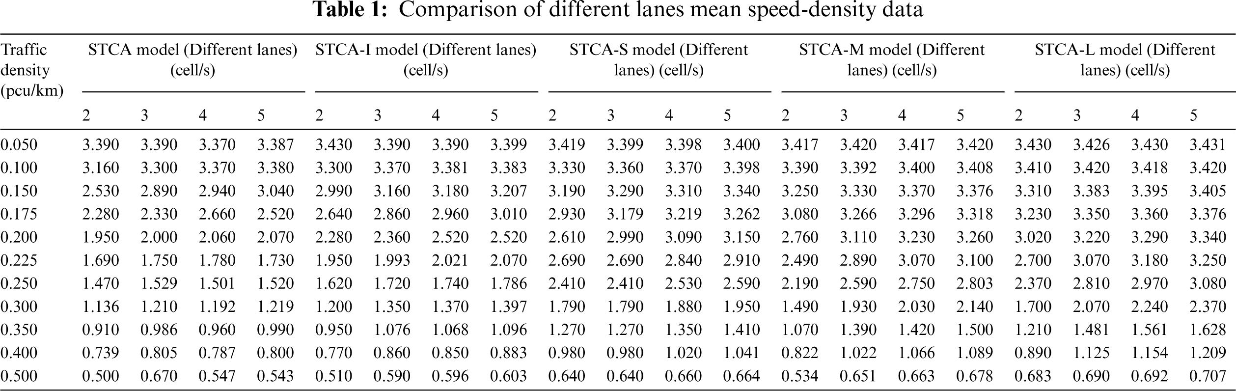
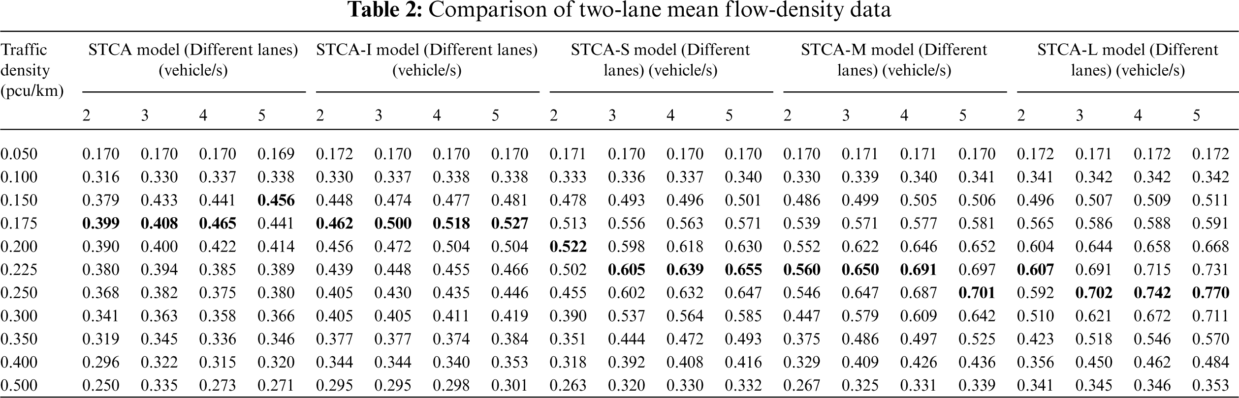
The data in Table 1 shows that the average speed value decreases with the increase of the vehicle density value, and the data in Table 2 shows that the average flow value increases rapidly as the vehicle density value increases. After reaching the maximum value, it decreases from steep to gentle, which conforms to the fundamental law of the three elements of traffic flow. We analyzed the specific data of the 4 lanes model in lanes 2, 3, 4, and 5 and found that: the area of maximum flow is within the range of [0.175, 0.250] pcu/km, the maximum flow of STCA and STCA-I under 2 lanes is at the vehicle density value of 0.175 pcu/km, which is 0.399 vehicles/s and 0.462 vehicles/s, respectively. The results are consistent with the numerical simulations in the literature [23]. The STCA-I model reflects the law of vehicle lane changing through the dynamic safety distance based on STCA, and the average traffic has a greater increase compared with STCA. The vehicle density of the STCA-S model reaches the maximum flow rate at 0.2 pcu/km, which is 0.522 vehicle/s. This shows that the cooperative lane change method of the model can increase the lane change frequency to ensure safe lane change while increasing road utilization. When the vehicle density is set to 0.225 pcu/km, the maximum average flow of the STCA-M model is 0.560 vehicles/s, which is 21.2% higher than the average flow of the STCA-I model and 7.27% higher than the STCA-S model. The maximum average flow of the STCA-L model under 2 lanes is 0.607 vehicles/s, which is 16.28% higher than STCA-S and 8.39% higher than the STCA-M model. The STCA-L model under 3 lanes is compared with STCA-S based on the maximum average flow by 16.03%, and compared with STCA-M by 8.00%. Under 4 lanes, the maximum average flow of the STCA-L model is increased by 16.12% compared with STCA-S and 7.38% compared with STCA-M. With the STCA-L model under 5 lanes, the maximum average flow is increased by 17.56% compared with STCA-S and 9.84% compared with STCA-M. Through the comparison of the Three-lane models, it is found that both the average speed and the average flow rate are increasing slightly. Because the STCA-L model considers the two-way lanes on both sides, it is more dominant in the average speed to achieve synergistic lane change without slowing down. The average flow under different lane numbers is effectively improved with the increased road capacity by incorporating collaborative lane changing and dynamic safety distance. In comparison to the STCA, STCA-I, STCA-S, and STCA-M models, this is a significant way to alleviate the growing burden on urban roads generated by the gradual growth of car ownership in the future with the expansion of the road and increase in the number of lanes.

According to Table 2, it provides that with the increase in the number of lanes, the growth trend of average flow is gradually decreasing. The growth rate is less than the growth rate of the physical space, i.e., when the 2 lanes are expanded to the 3 lanes, the physical space is expanded by 50%, and the growth rate of the average flow is 15.65%. Similarly, if the three-lanes are expanded to 4 lanes, the physical space is expanded by 33.33%, and the average flow growth rate is 5.67%, and when the 4 lanes are expanded to 5 lanes, the physical space is expanded by 25%, and the average flow growth rate is 3.77%. Through the comparison of specific data, the growth rate of the average traffic is continuously decreasing. It shows that the exponential growth of physical space cannot bring about a corresponding increase in average flow. Therefore, an appropriate increase in the number of lanes can effectively increase the average flow, while an unlimited increase in the number of lanes cannot increase the average flow more significantly.

4.2 Time-Space Diagram Analysis

We are considering the basic graph curves of the 5 models in the traffic flow pictures. In the experiment, the traffic density at locations with significant differences in average flow is 0.225 pcu/km. The space-time diagrams of lanes 2, 3, 4, and 5, respectively, are plotted as shown in Table 3.

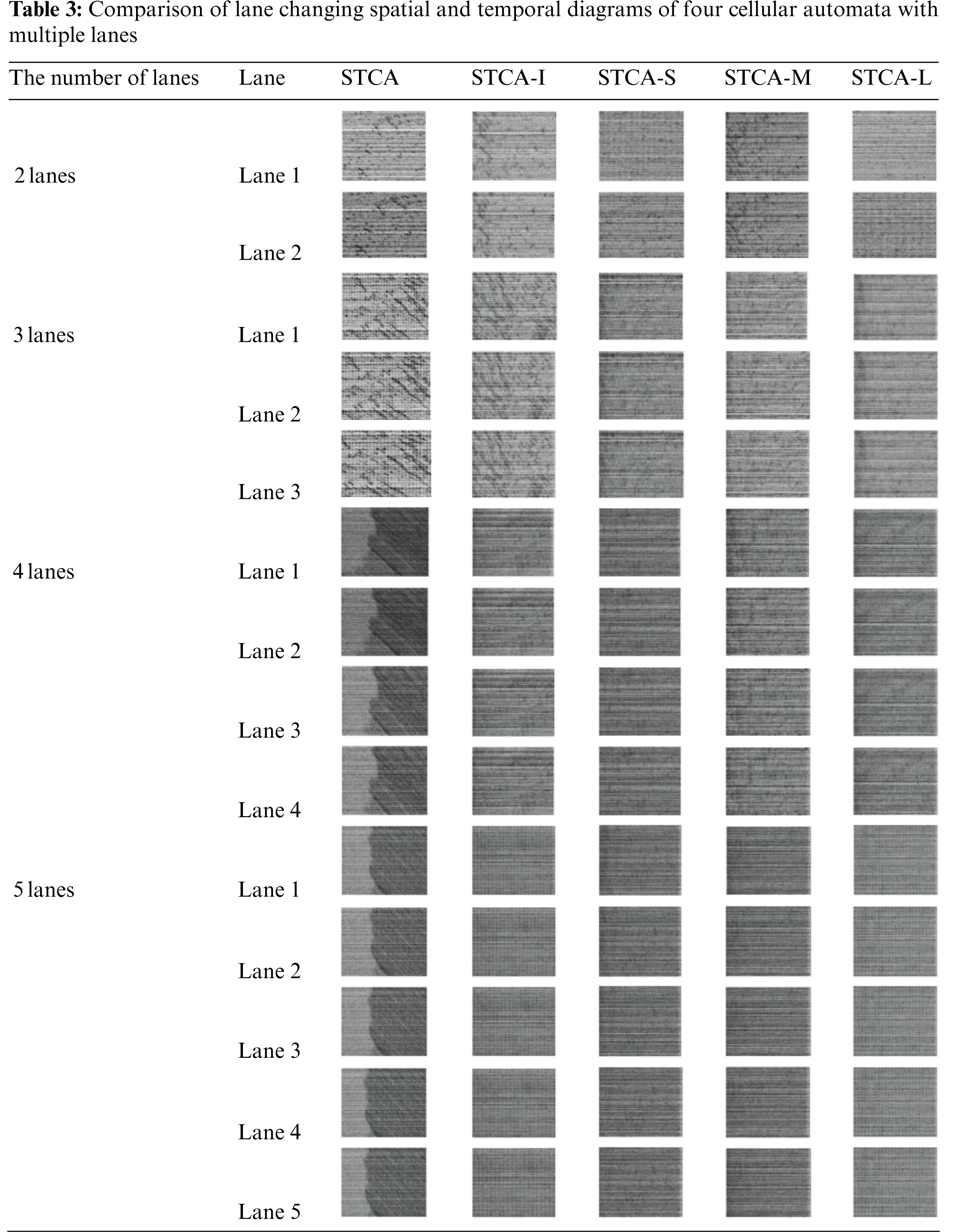
The vehicle density for all the models in Tables 2 and 3 is set to 0.225 pcu/km. The average flow value of the STCA model and the STCA-I model is not the maximum value of the model at the entering area where there is a possibility of a traffic jam. We observe from the STCA model time-space diagrams of the STCA and STCA-I models reduce the possibility of lane changing due to the safety distance requirement. This method reduces the available road resources. The lane change rate will drop rapidly as the number of vehicles increases. It can be seen that the formation of patches due to traffic jams in the STCA model has accumulated over time without obvious dissipation, especially in the 4 and 5 lanes, i.e., the model does not play a good role in regulating vehicles in a multi-lane environment. Although the STCA-I model has fewer patches than the STCA model, it is still because the above 2 models used passive lane-changing simulations and lack active lane-changing guidance. The jammed patches in the time-space map dissipate slowly, which form a backward transmission. The STCA-L, STCA-S and STCA-M have used active lane-changing guidance and speed guidance under the same vehicle density conditions. It can be found that there are fewer jammed patches as compared with the previous two models STCA and STCA-I. In particular, compare the number and dissipation process of patches in the 4 and 5 lanes of the STCA-L model, the model with active lane change guidance can quickly drive the patches to dissipate. Although the four-lane jam tends to transfer to the upstream, after several iterations, the jam dissipated. For the area with the slower speed in 5 lanes, there is no upstream propagation effect. This is because a more reasonable threat evaluation is set for lane-changing behavior, which reduces the error rate of the driver's subjective judgment about the safety distance and increases the success rate of lane-changing. At the same time, the introduction of speed guidance based on jam points can make the road driving of the vehicle predictable under the condition of active guidance. The increase in synchronous vehicle speeds further reduces the dissipating time of the jam point and reduces the deceleration and start-stop behavior of upstream vehicles due to the jam point. We can see from the STCA-L model in the space-time diagram of different lane numbers, and the vehicles gradually become synchronized under this model's lane-changing guidance. It shows that under the conditions of vehicle-road cooperative information interaction, effective guidance on the speed of lane-changing vehicles can change road vehicles and improve road usage efficiency and methods.

4.3 Vehicle Density and Lane Changing Frequency

Fig. 5 shows the channel shift frequency of various evolving models ranging from 0.1 to 0.7 pcu/km vehicle density values in 2, 3, 4, and 5 lanes road settings.

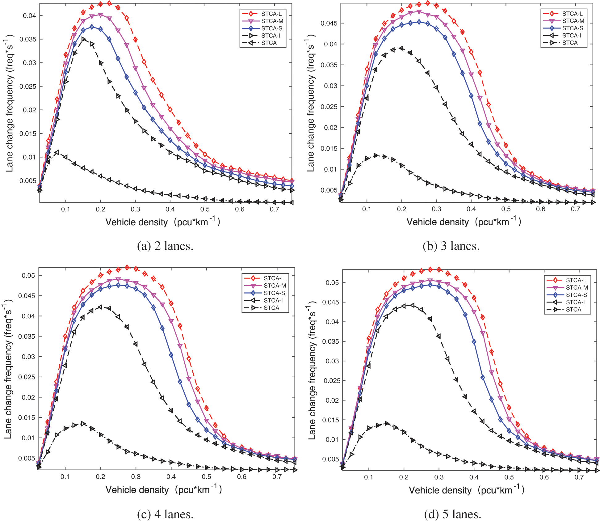
Figure 5: Comparison diagram of multi-lane lane changing frequency of 5 models

We compare the lane change frequency of the 5 models and found that: In the low-density interval of the vehicle, i.e., [0, 0.1] pcu/km range. Because of the low vehicle density and adequate free space, vehicles need fewer lane changes and can adapt to their driving at their own speed. Even if lane-changing is needed, the safe lane-changing distance is adequate for the vehicle to change lanes safely. Therefore, there is not much difference between the 5 models in the low vehicle density range. With the further increase of the vehicle density, the lane-changing situation gradually makes a difference. We analyzed the vehicle density at [0.1, 0.25] pcu/km range. As density grew, blocked vehicles became more prevalent, and the demand for vehicle lane changes steadily increased, as did the frequency of lane changes. In the density interval of [0.25, 0.4] pcu/km, except for the STCA-L model, the lane-changing frequency corresponding to the other models begins to decrease. The STCA-L lane changing rules are flexible, and the lane changing rate can still be maintained in this interval. However, when the vehicle density reaches 0.5 pcu/km, the lane-changing frequency decreases rapidly. It is difficult to quantify the benefit of coordinated lane changes due to the compression of the physical space of the road. In Fig. 5, except for the STCA model's lane-changing frequency curve, the changing trend of the lane-changing frequency and the numerical value of the other 4 models are less different.

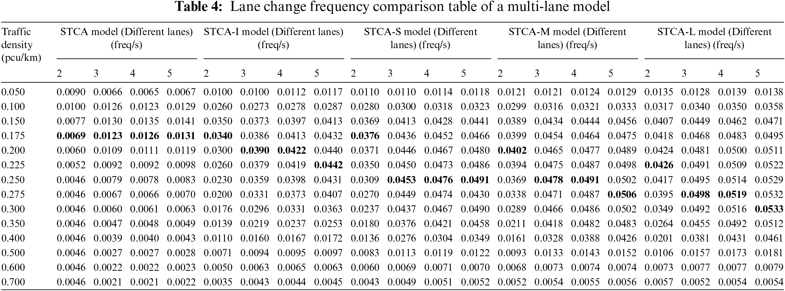
By comparing the results shown in Table 4 and Fig. 5, we determined that the vehicle density corresponding to the STCA-L model's maximum lane changing frequency is 0.275 pcu/km in 3 and 4 lanes and 0.300 pcu/km in 5 lanes. As the number of lanes increases, the maximum value of lane-changing frequency shifts to a higher density interval. However, once the vehicle density exceeds 0.400 pcu/km, road congestion is inevitable, and the model's adjustment impact is lost. STCA-I and STCA-S have reflected the same trend of change. The vehicle density corresponding to each model's maximum lane change frequency is the same as the average flow corresponding value. The STCA model's slightly lower lane change frequency is due to its overly stringent criteria for inter-vehicle spacing. The lane changing frequency trend corresponding to the STCA model is consistent with STCA-S, STCA-M, and STCA-L, but it only represents the actual lane changing frequency in the current environment. STCA-S introduces the concept of vehicle-road coordination with the frequency of lane changes increased to a certain extent. STCA-L takes the overall consideration of the road section according to the threat of surrounding vehicles combined with the information of jammed road section and provides the safe lane changing conditions for vehicles as far as possible. Therefore, lane changing frequency corresponding to the maximum lane changing the frequency of STCA-I model, STCA-S model and STCA-M model increases by 20.18%, 11.73% and 5.63%, respectively the 2 lanes. Under the 3 lanes, an increase by 21.68%, 9.04% and 4.02%, respectively. Similarly, under 4 lanes, it increased by 18.68%, 8.28% and 5.39%, and 17.07%, 7.88%, and 5.06% under 5 lanes. For the STCA-L model, the lane-changing frequency of the 3 lanes model is 16.90% higher than that of 2 lanes model, 4 lanes model is 4.20% higher than that of 3, and 5 lanes model is 2.69% higher than that of 4 lanes model. If 4 lanes are extended to 5, then the maximum lane frequency growth rates change for the STCA-I, STCA-S, and STCA-L models are 4.52%, 3.05%, and 2.63%, respectively, with the STCA-L model having a lower maximum lane change frequency growth rate.

The growth rate of lanes is constantly decreasing, and it is much lower than the growth rate of lanes. When 4 lanes are expanded to 5 lanes, the growth rates of STCA-I, STCA-S and STCA-L models maximum lane change frequency are 4.52%, 3.05% and 2.63%, respectively, and the STCA-L model has a lower overall lane change frequency growth rate than the STCA-I and STCA-S models. The above analysis shows that the lane changing model based on driving guidance proposed in this paper can further explore the possibility of vehicle lane changing and improve road use efficiency. Increased lanes reduce the physical space available for lane changes and allow for further lane changes. Lanes are possible, but the rise in lane-changing frequency indicates that infinitely widening lanes cannot significantly increase lane-changing frequency.

4.4 Analysis of Induced Speed Compliance Rate

Based on the current usage of navigation software, it can be predicted that at the initial stage of vehicle-road collaborative information sharing, the vehicle operation guidance will also be completed by the driver. Whether the driver can comply with the driving guidance information will affect traffic flow in the road section. Therefore, in this section, we will discuss the effectiveness of the model under different compliance rates. In this paper, the relationship between average speed, flow and vehicle density is analyzed according to different compliance conditions. STCA-L lane change guide speed compliance rate value, pc=0.1,0.3,0.5,0.7,0.9,0.95. The reason for setting the full compliance rate at 0.95 is that even with total compliance driving instructions, there is still a risk of failing to comply with lane changing instructions due to vehicle malfunction, making it difficult to comply with driving instructions 100% in the case of complete driverless driving. Suppose there is a 0.05 non-compliance with the set rule. Figs. 6–9 compare the average vehicle speed and flow obtained with various enforcement rates and vehicle densities under various lane numbers.

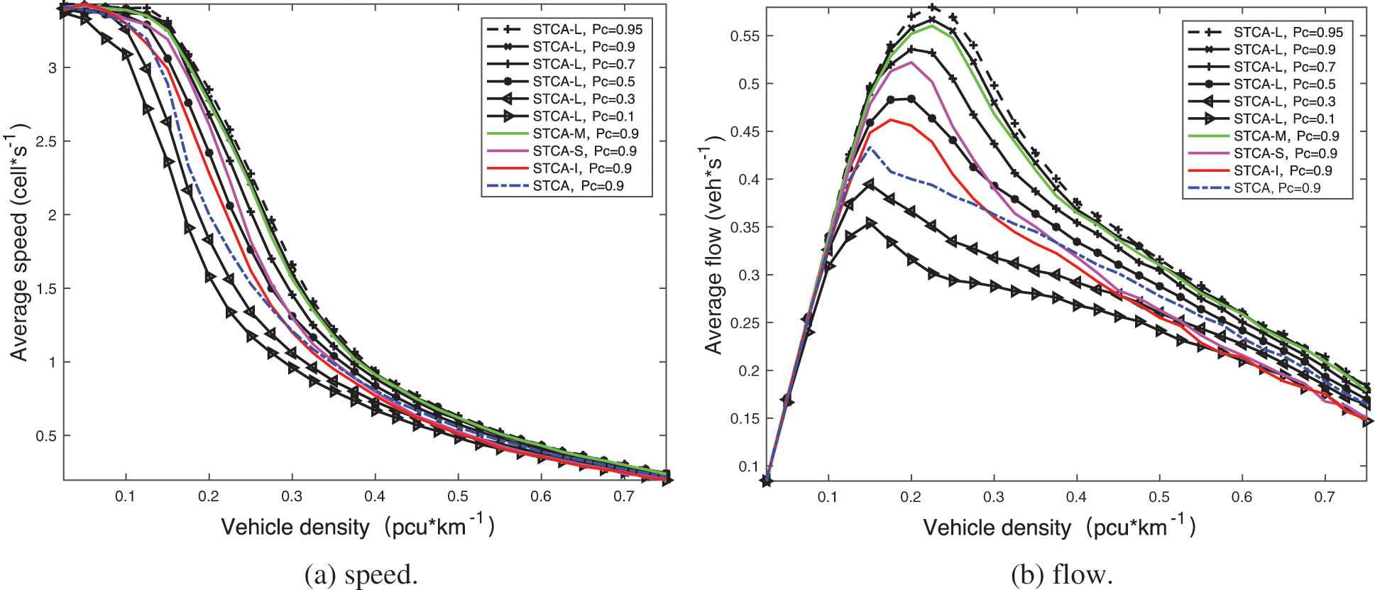
Figure 6: Basic diagram of 2 lanes speed and flow under different induced vehicle speed compliance rates

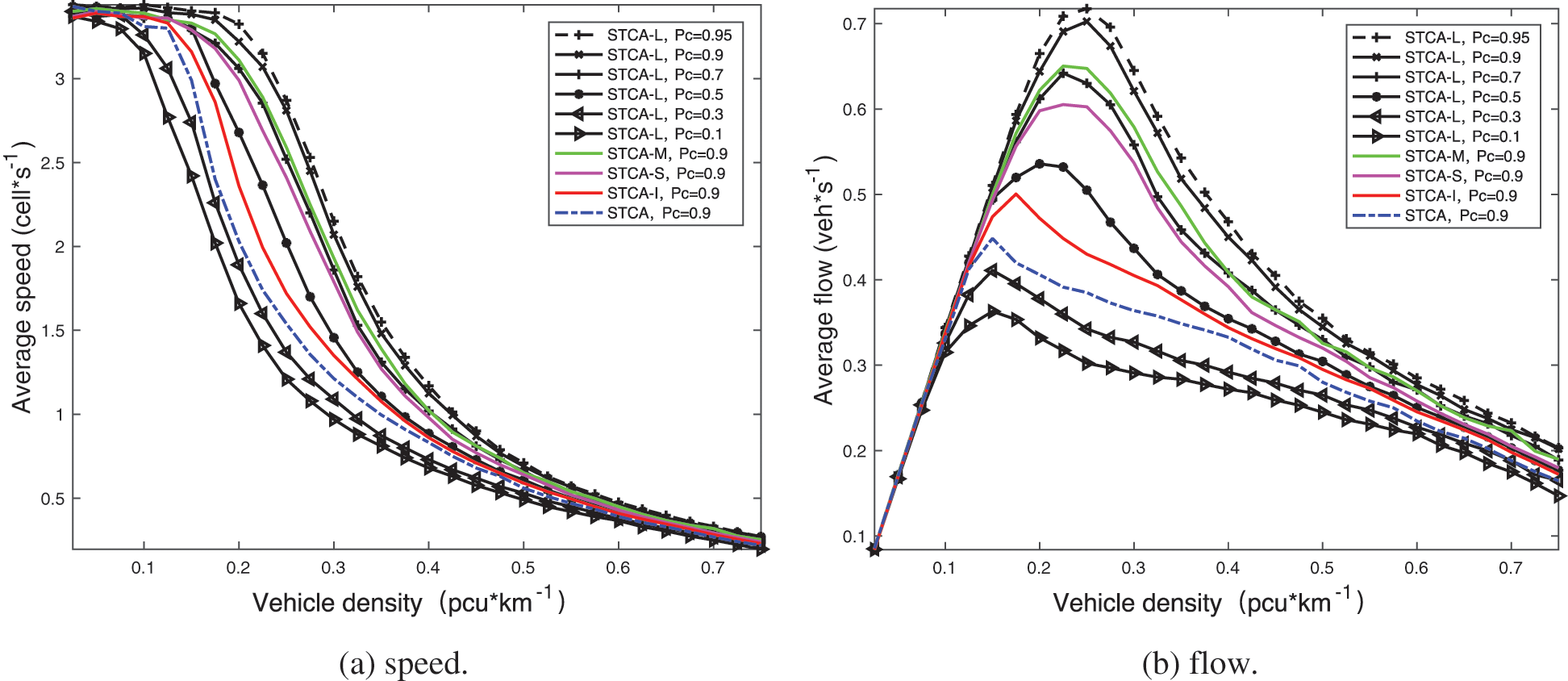
Figure 7: Basic diagram of 3 lanes speed and flow under different induced vehicle speed compliance rates

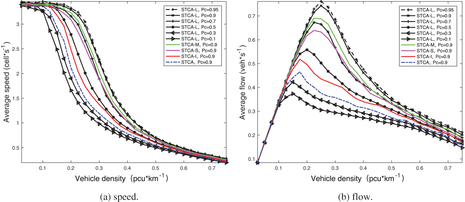
Figure 8: Basic diagram of 4 lanes speed and flow under different induced vehicle speed compliance rates

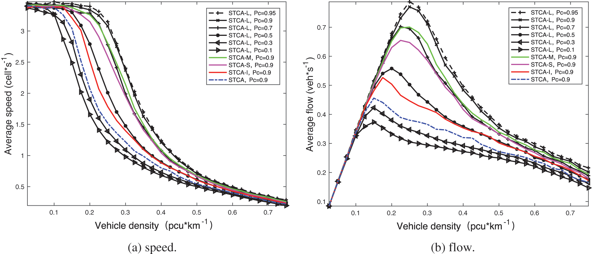
Figure 9: Basic diagram of 5 lanes speed and flow under different induced vehicle speed compliance rates

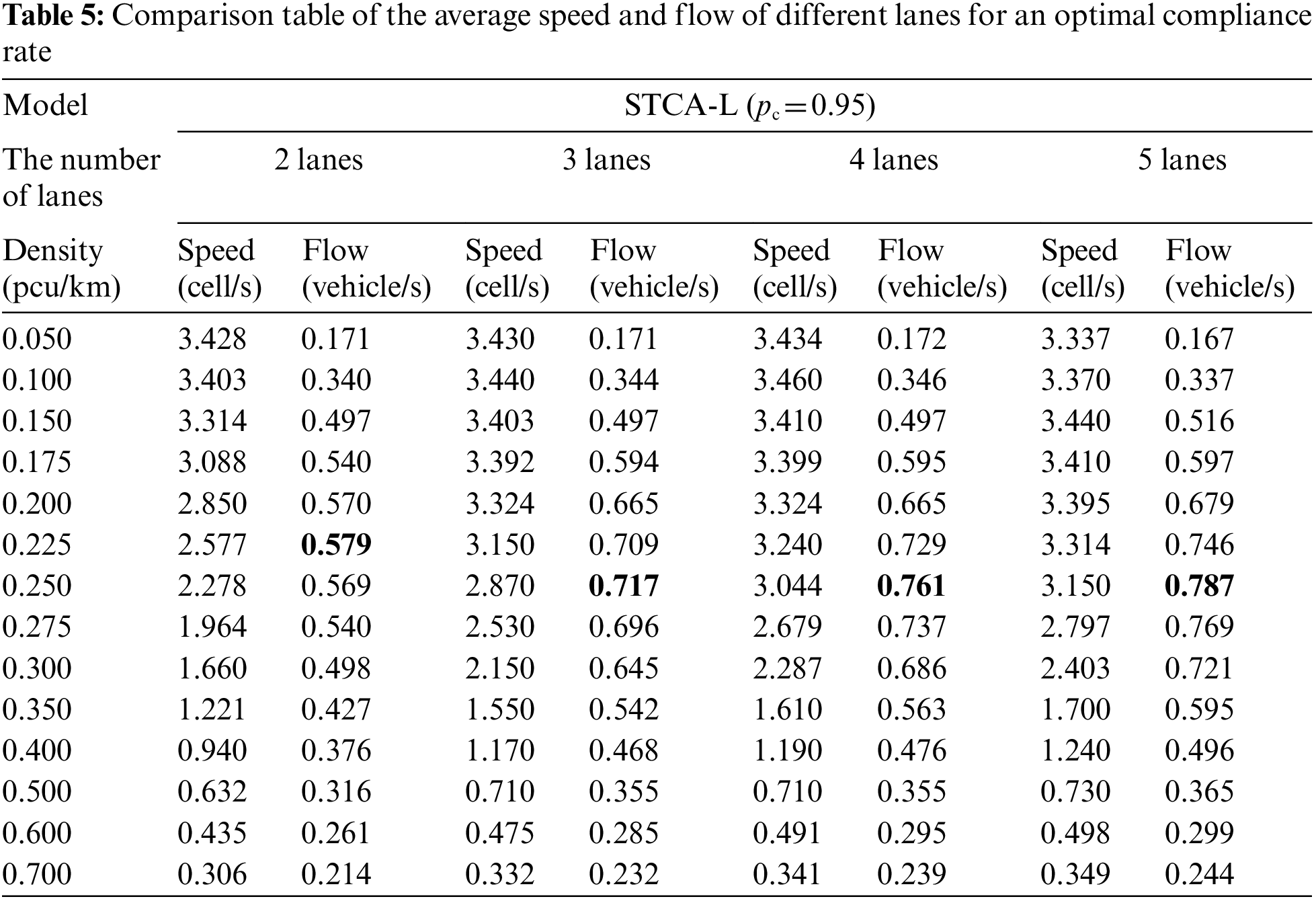
Figs. 6–9 show that when the compliance rate is 0.95, all vehicles can be controlled by lane changing and speed according to the guidance, and the optimal average flow can be obtained. Referring to Table 2, when the vehicle density is 0.225 pcu/km, the average flow reaches the maximum value of 0.607 veh/s. When the compliance rate decreases, the corresponding average flow value decreases together. When the compliance rate is less than 0.7, the vehicle density value corresponding to the maximum average flow of STCA-L is the same as STCA-M and STCA-S, and the corresponding traffic flow change trend is similar. Where the compliance rate is less than 0.6, the impact on average flow is not as strong as with the STCA-M model. When the compliance rate is 0.45, it is the same as the maximum average flow of STCA-I. When the compliance rate is less than 0.3, the lane-changing advantage of STCA-L cannot be reflected, and even the utilization effect of the road becomes worse due to the excessively free vehicle control mode.

Let critically analyze Figs. 6–9b and Table 5. The maximum average flow rate for a given number of lanes is approximately 0.225 pcu/km. If the vehicle density is greater than 0.5 pcu/km, then the change in the compliance rate of the STCA-L model did not result in a significant change in the average traffic under high vehicle density road conditions. The change of compliance rate of the STCA-L model does not lead to an effective change in the average traffic flow under high vehicle density road conditions.

In the road dominated by jammed flow, there are fewer control modes that can provide the vehicles with free choice, i.e., the vehicles are required to comply with lane changing rules objectively. Therefore, in the environment of high vehicle density, the STCA-L model presented in this paper can gain a slight advantage in the average flow value. Through the above analysis, the STCA-L model can better regulate traffic flow under various compliance rates. Compared with the other 4 models, our proposed model is more suitable for future urban vehicle-road coordination roads.

5  Conclusion

In this paper, an improved STCA multi-lane lane-changing model based on driving guidance is introduced. We evaluate vehicles’ operating status and mutual impact in a multi-lane environment using the interactive information content of vehicles and roads generated by vehicle-road collaboration. This paper focuses on the establishment of lane change guidance and speed induction functions for driving vehicles’ in local areas of disturbance and builds the STCA-L cooperative lane change model by integrating the NS-S model and the STCA-S update mode. Finally, numerical simulation is performed using the actual multi-lane traffic conditions.

Several experiments are executed to compared STCA, STCA-I, STCA-S, STCA-M, STCA-L models performance efficiency. According to the average flow value, the model presented in this paper increases the number of vehicles on the road and improves traffic flow over a broader range of vehicle densities. Compared with the STCA-S model under 2, 3, 4, and 5 lanes, the average flow value increases to 16.28%, 16.03%, 16.12%, and 17.56%, respectively. Similarly, compared with the STCA-M model under 2, 3, 4, and 5 lanes, the average flow value increases to 8.39%, 8.00%, 7.38%, and 9.84%, respectively. The time-space diagram analysis proved that the model in this paper has a good driving guidance function, effectively reducing the “start-stop” of the vehicle, and the synchronization phase is increased. It can be seen from the lane change rate curve that the lane change rules in this paper are more flexible and can give more lane changing opportunities under the premise of safety. Finally, the STCA-L coordinated lane change model is compared and analyzed under different lane numbers. It can be seen that the infinite widening of lanes does not bring more traffic, indicating that the model's adjustment to the road does not depend on the increase of the physical space of the road. However, at the same time, the proposed method in this paper gives the assumption of information interaction under the vehicle-road system, with the compliance rate having a greater impact on the guidance effect of the model. In addition, the increase in the amount of instantaneous information is suitable for human driving conditions. In future work, we shall study the instantaneous information that can suit the human driving condition.

Funding Statement: This work was supported in part by the National Natural Science Foundation of China (No. 51905405), Basic Research Program of Natural Science of Shaanxi Province (No. 2022JM-407), Guiding Program of Science and Technology of China Textile Industry Federation (No. 2020106).

Conflicts of Interest: The authors declare that they have no conflicts of interest to report regarding the present study.

References

 1.  Zhang, L., Zhu, X. T., Li, J. Y. (2020). Research on application of network slices in vehicle-road cooperative system. Application of Electronic Technique, 46(1), 12–16. DOI 10.16157/j.issn.0258-7998.191362. [Google Scholar] [CrossRef]

 2.  Cui, X. W. (2018). Vehicle-road collaboration creates the future--Discussion on the application of intelligent highway technology in vehicle-road collaboration. Traffic Informatization in China, 225(12), 22–26. DOI 10.13439/j.cnki.itsc.2018.12.002. [Google Scholar] [CrossRef]

 3.  Chen, C., Lu, Z. Y., Fu, S. S., Peng, Q. (2011). Overview of the development in cooperative vehicle-infrastructure system home and abroad. Journal of Transportation Information and Safety, 29(1), 102–105. [Google Scholar]

 4.  Yao, Z., Xu, T., Jiang, Y., Hu, R. (2021). Linear stability analysis of heterogeneous traffic flow considering degradations of connected automated vehicles and reaction time. Physica A: Statistical Mechanics and its Applications, 561, 125218. DOI 10.1016/j.physa.2020.125218. [Google Scholar] [CrossRef]

 5.  Hua, X. D., Wang, W., Wang, H. (2016). A car-following model with the consideration of vehicle-to-vehicle communication technology. Acta Physica Sinica, 65(1), 13–25. DOI 10.7498/aps.65.010502. [Google Scholar] [CrossRef]

 6.  Wu, Z. J. (2009). Volvo introduces city safety system. Light Vehicles, 3, 25. [Google Scholar]

 7.  Zhang, L. W. (2015). Laying the groundwork for autonomous driving Honda SENSING & Honda CONNECT. Auto Fan, 23, 108–111. [Google Scholar]

 8.  Rasheed, I., Hu, F., Hong, Y. K., Balasubramanian, B. (2021). Intelligent vehicle network routing with adaptive 3D beam alignment for mmWave 5G-based V2X communications. IEEE Transactions on Intelligent Transportation Systems, 22(5), 2706–2718. DOI 10.1109/TITS.2020.2973859. [Google Scholar] [CrossRef]

 9.  Chao, Z., Zhan, L. (2021). Research on the application of cloud side cooperation technology in urban rail transit video surveillance system. Railway Transportation and Economy, 106–110. [Google Scholar]

10. Lee, S., Ngoduy, D., Keyvan-Ekbatani, M. (2019). Integrated deep learning and stochastic car-following model for traffic dynamics on multi-lane freeways. Transportation Research Part C: Emerging Technologies, 106(9), 360–377. DOI 10.1016/j.trc. [Google Scholar] [CrossRef]

11. Lombard, A., Abbas-Turki, A., El-Moudni, A. (2020). V2v-based memetic optimization for improving traffic efficiency on multi-lane roads. IEEE Intelligent Transportation Systems Magazine, 12(1), 35–46. DOI 10.1109/mits.2018.2879183. [Google Scholar] [CrossRef]

12. Zhou, B., Wang, Y., Yu, G. (2017). A lane-change trajectory model from drivers’ vision view. Transportation Research Part C: Emerging Technologies, 85(12), 609–627. DOI 10.1016/j.trc.2017.10.013. [Google Scholar] [CrossRef]

13. Li, T. T., Wu, J. P., Chan, C. Y. (2020). A cooperative lane change model for connected and automated vehicles. IEEE Access, 8, 54940–54951. DOI 10.1109/access.2020.2981169. [Google Scholar] [CrossRef]

14. Yao, Z., Jiang, H., Cheng, Y., Jiang, Y., Ran, B. (2020). Integrated schedule and trajectory optimization for connected automated vehicles in a conflict zone. IEEE Transactions on Intelligent Transportation Systems. DOI 10.1109/TITS.2020.3027731. [Google Scholar] [CrossRef]

15. Laarej, A., Karakhi, A., Khallouk, A. (2020). Dissipation energy and satisfaction rate for a two-lane traffic model with two types of vehicles. Chinese Journal of Physics, 71, 2221. DOI 10.1016/j.cjph.2020.05.024. [Google Scholar] [CrossRef]

16. Wang, Z., Zhao, X., Xu, Z. (2019). Modeling and field experiments on lane changing of an autonomous vehicle in mixed traffic. Autonomous Vehicles. DOI 10.13140/RG.2.2.19857.58724. [Google Scholar] [CrossRef]

17. Ma, Y., Zhang, P., Hu, B. (2019). Active lane-changing model of vehicle in B-type weaving region based on potential energy field theory. Physica A: Statistical Mechanics and its Applications, 535(1), 122291. DOI 10.1016/j.physa.2019.122291. [Google Scholar] [CrossRef]

18. Tang, T. Q., Shi, W. F., Shang, H. Y. (2014). An extended car-following model with consideration of the reliability of inter-vehicle communication. Measurement, 58(11), 286–293. DOI 10.1016/j.measurement.2014.08.051. [Google Scholar] [CrossRef]

19. Fakirah, M., Leng, S., Chen, X. (2020). Visible light communication-based traffic control of autonomous vehicles at multi-lane roundabouts. EURASIP Journal on Wireless Communications and Networking, 2020(1). DOI 10.1186/s13638-020-01737-x. [Google Scholar] [CrossRef]

20. Lu, N., Wang, H., Wang, K., Liu, Y. (2021). Maximum probabilistic and dynamic traffic load effects on short-to-medium span bridges. Computer Modeling in Engineering & Sciences, 127, 345--360. DOI 10.32604/cmes.2021.013792. [Google Scholar] [CrossRef]

21. Deng, J. H., Feng, H. H., Ge, T. (2019). Conflict handing strategies of lane-changing decision model of multi-lane cellular automata. Journal of Transportation Systems Engineering and Information Technology, 19(4), 50–54. [Google Scholar]

22. Hou, J. (2018). The traffic characteristics and capacity analysis method for diverge influence arear on multi-lane freeways (Ph.D. Thesis). Southeast University, China. [Google Scholar]

23. Tan, M. C. (2009). Nonlinear optimal control model of multi-lane traffic flow. Computer Engineering and Applications, 45(13), 13–15. DOI 10.3778/j.issn.1002-8331.2009.13.004. [Google Scholar] [CrossRef]

24. Wolfram, S. (1983). Statistical mechanics of cellular automata. Reviews of Modern Physies, 55, 601–644. DOI 10.1103/RevModPhys.55.601. [Google Scholar] [CrossRef]

25. Nagel, K., Schreckenberg, M. (1992). A cellular automaton model for freeway traffic. Journal De Physique I France, 2(12), 2221–2229. DOI 10.1051/jp1:1992277. [Google Scholar] [CrossRef]

26. Chowdhury, D., Wolf, D. E., Schreckenberg, M. (1997). Particle hopping models for two-lane trafic with Two kinds of vehicles: Effects of lane-changing rules. Physica A: Statistical Mechanics and its Applications, 235(3), 417–439. DOI 10.1016/S0378-4371(96)00314-7. [Google Scholar] [CrossRef]

27. Wang, Y. M., Zhou, L. S., Lu, Y. B. (2008). Lane changing rules based on cellular automata traffic flow model. China Journal of Highway and Transport, 21(1), 89–93. DOI 10.3321/j.issn:1001-7372.2008.01.016. [Google Scholar] [CrossRef]

28. Jian, M., Li, X., Cao, J. (2020). Investigating model and impacts of lane-changing execution process based on CA model. International Journal of Modern Physics C, 31(12). DOI 10.1142/S0129183120501715. [Google Scholar] [CrossRef]

29. The State Council of the PRC (2017). The development plan of modern integrated transport system during the 13th five-year plan period. iChina, 3, 18. [Google Scholar]

30. Xu, H. X., Chu, S. F. (2016). A symmetric same direction two-lane trafic flow model based on safe lane changing distance rule. Journal of Shenyang University (Natural Science), 28(2), 118–121. [Google Scholar]

31. Li, X., Qu, S. R., Xia, Y. (2014). Cooperative lane-changing rules on multilane under condition of cooperative vehicle and infrastructure system. China Journal of Highway and Transport, 27(8), 97–104. [Google Scholar]

32. Li, X., Ma, W. Z., Zhao, Z. F., Zhang, K. B., Wang, X. H. (2020). Improved STCA lane changing model for two-lane road based on driving guidance under CVIS. Journal of Southeast University (Natural Science Edition), 50(6), 1134–1142. DOI 10.3969/j.issn.1001-0505.2020.06.021. [Google Scholar] [CrossRef]

33. Shi, B., Li, X., Nie, T., Zhang, K., Wang, W. (2021). Multi-object recognition method based on improved YOLOv2 model. Information Technology and Control, 50(1), 13–27. DOI 10.5755/j01.itc.50.1.25094. [Google Scholar] [CrossRef]

34. Li, X., Zhao, F. Z., Liu, Y., Nan, K. K. (2018). An improved NS model for single lane with induce speed under situation of cooperative vehicle infrastructure system. Journal of Highway and Transportation Research and Development, 35(2), 101–108. DOI 10.3969/j.issn.1002-0268.2018.02.014. [Google Scholar] [CrossRef]

35. Li, X. (2015). Research on microscopic traffic guidance and control for multi-lane on cooperative vehicle infrastructure environments (Ph.D. Thesis). Northwestern Polytechnical University, China. DOI 10.7666/d.D689468. [Google Scholar] [CrossRef]

36. Wang, Y. M. (2010). Study of traffic congestion's simulation based on cellular automaton model. Journal of System Simulation, 9, 2149–2154. [Google Scholar]

This work is licensed under a Creative Commons Attribution 4.0 International License, which permits unrestricted use, distribution, and reproduction in any medium, provided the original work is properly cited.