Computer Modeling in Engineering & Sciences

---

DOI: 10.32604/cmes.2022.021235

ARTICLE

Optimization Analysis of the Mixing Chamber and Diffuser of Ejector Based on Fano Flow Model

Lixing Zheng1,*, Weibo Wang2, Yiyan Zhang1, Lingmei Wang3 and Wei Lu2

1School of Electric Power, Civil Engineering and Architecture, Shanxi University, Taiyuan, 030006, China
2School of Mechanical Engineering, Guangxi University, Nanning, 530004, China
3Wind Turbine Monitoring and Diagnosis, NTRC of Shanxi Province, Taiyuan, 030006, China
*Corresponding Author: Lixing Zheng. Email: lxzheng@sxu.edu.cn
Received: 03 January 2022; Accepted: 09 February 2022

Nomenclature

A	cross-sectional area (m2)
cp	specific heat at a constant pressure (kJ/kg⋅K)
D	diameter (m)
f	coefficient of friction
k	adiabatic index
L	length (m)
m˙	mass flow rate (g/s)
Ma	Mach number
NXP	position of the nozzle exit
p	pressure (MPa)
r	radius (m)
Re	Reynolds number
T	temperature (oC)
T*	total temperature (oC)
V	velocity (m/s)
x	distance to section 2 (m)
y	velocity ratio

Greek symbols

α	semi-cone angle of the diffuser
η	efficiency
θ	semi-cone angle of the mixing chamber
μ	entrainment ratio or viscosity coefficient

Subscripts

c	outlet diameter of the diffuser
c3	mixing chamber at section 3
ce	experimental value of the diffuser outlet
cn	mixing chamber at section n
d	diffuser
e	secondary flow
e2	secondary flow in section 2
g	primary flow
g0	throat of the motive nozzle
g1	primary flow in section 1
g2	primary flow in section 2
m	mixing chamber
m1	length of the mixing section
m2	length of the mixed section
n	throat of the nozzle
s	shock wave
z	distance to section 3

1  Introduction

Compared to conventional mechanical supercharging equipment (compressors, pumps, and blowers), ejectors have lower energy consumption and a simpler structure. Ejectors have been used in the refrigeration system to recover the energy of the high-pressure fluid and reduce the power of the compressor to improve the circulation efficiency of the system [1]. In addition, ejectors have been widely used in the nuclear industry [2], chemical industry [3], aerospace industry [4], thermal-power generation [5], and food drying [6].

Nevertheless, the flow characteristic of the ejector is complicated due to non-equilibrium, entrainment, condensation, collision, and friction. Many scholars have carried out steady-state simulations, computational fluid dynamic (CFD) analyses, and experimental tests to investigate the performance of the ejector. Especially, CFD-based simulation and analysis can provide detailed information on the flow field [7]. Peng et al. [8] built a three-dimensional CFD model to analyze the influence of the distance of the standoff from the nozzle outlet on the performance of a high-speed rotating water ejector. Wang et al. [9] proposed a control method to reduce non-equilibrium condensation in the motive nozzle of the ejector. Yang et al. [10] used a CFD model to investigate the non-equilibrium condensation of steam in the supersonic ejector. An accurate analysis of a non-equilibrium flow can optimize the motive nozzle of the ejector. Moreover, except for understanding the local flow characteristic, the whole flow properties of ejector are more necessary and important. Wu et al. [11] used a CFD model to analyze the effects of the following parameters on the distribution of flow fields in the ejector: the diameter of the outlet of the motive nozzle, position of the nozzle exit (NXP), diameter of the contraction section of the mixing chamber, and diameter of the diffuser. Nakagawa et al. [12] conducted experimental studies on the flow structure of the ejector, and pointed out that the length of the mixing section affects not only pressure recovery but also entrainment ratios. Dong et al. [13] established a three-dimensional numerical model to investigate the effect of the length of mixing chamber on the performance of steam ejector under different degrees of the Mach number in nozzle exit, the length of constant-area section and the length of diffuser. The results showed that the mixing chamber plays an important role in the performance of the ejector.

The function of the mixing chamber of the ejector is to mix the two fluids of the primary flow and secondary flow and ensure momentum and heat transfer [14]. Avila et al. [15] proposed a novel MLPG–finite volume method to obtain accurate pressure and velocity fields of the mixing flow. Zhu et al. [16] used CFD analysis to investigate the influence of the convergence angle of the mixing chamber on the mixing effect of the ejector. Wu et al. [17] studied the effects of the length and convergence angle of the mixing chamber on the performance of the ejector. Fu et al. [18] proposed a method to optimize the diameter of the mixing chamber. Abdel-hamid et al. [19] added a tail section to the mixing chamber of the ejector and studied the influence of the diameter of the tail section on the performance of the ejector. Serra-Pallares et al. [20] developed a method to optimize the conical mixing chamber of the ejector. Chen et al. [21] proposed a method to design a cylindrical mixing chamber on the basis of actual gas characteristics. Ameur et al. [22] carried out an experimental study to analyze the influence of the mixing chamber and diffuser on the performance of the ejector under different working conditions. The function of the diffuser is to convert the kinetic energy of the mixed fluid into pressure energy. Yuan et al. [23] researched the effect of the expansion range of the diffuser on the performance of the ejector. Elbel et al. [24] experimentally tested different diffuser angles and concluded that when the diffuser angle was 5°, the diffuser showed the best performance. However, Banasiak et al. [25] conducted experimental and numerical assessments of the expansion range of the diffuser, and found that 3° was the best expansion angle of the diffuser. Therefore, previous studies have shown that the expansion angle and length of the diffuser have an important influence on the pressure lift of the ejector. The suboptimal expansion angle and length of the diffuser are detrimental to the performance of the ejector.

Although there are many studies on the geometry of the ejector, there are few studies on the radial dimensions of the ejector. The axial dimensions of the ejector, including the position of the nozzle exit, length of the mixing chamber, and length of the diffuser are rarely studied on the basis a sound theoretical model [26]. In particular, the length of the mixing chamber, which is important to momentum and heat transfer, should be given more attention. At present, the length of the mixing chamber and that of the diffuser are mainly determined using the empirical formula obtained on the basis of experimental data [27]. However, the empirical formula may not be applicable to different working conditions and working media. The flow of a fluid in the mixing chamber shares many similarities to the Fano flow, which describes the adiabatic flow in a constant-section channel and considers the effect of friction. Thus, a theoretical method can be proposed on the basis of the Fano flow theory to determine the axial dimensions of the mixing chamber.

In this paper, we established a model to calculate the length of mixing chamber on the basis of the Fano flow. An improved method that considers fluid friction and cross-sectional flow variation was proposed to determine the length of the diffuser. To verify the model validity, we compared the theoretical results calculated using the model to experimental data reported in literature. The influence of the outlet temperature Tc and outlet pressure pc of the ejector, expansion ratio (the pressure of the primary flow to that of the secondary flow pg/pe), and diameter ratio (the diameter of the throat of the motive nozzle to the diameter of the mixing chamber dg0/dc3) on the length of the mixing chamber Lm was analyzed. Moreover, the influence of the diffuser length Ld on the semi-cone angle of the diffuser α and diameter ratio (the outlet diameter of diffuser to the diameter of mixing chamber dc/dc3) was discussed.

2  Mathematical Models

2.1 Mathematical Models of the Mixing Chamber

There were seven key assumptions made to derive the ejector model. First, the fluid flow was a one-dimensional steady flow, and the expansion, compression, and mixing processes were adiabatic. Second, the primary flow was in a stagnant state at the inlet of the ejector and a choked state at the throat of the motive nozzle. Third, the secondary flow was in a stagnant state at the inlet of the suction chamber and a choked state at the inlet of the mixing chamber (Section 2, Fig. 1). Fourth, the velocity of the diffuser outlet was ignored. Fifth, the mixing of the primary flow and secondary flow began in Section 2, and constant pressure was maintained in the mixing chamber (pg2 = pe2). The mixing of the primary flow and secondary flow was completed in section n. Sixth, positive shock waves occurred in Section 3 of the mixing chamber. Seventh, the friction between steam and the tube wall was considered, and the coefficients of friction in the mixing chamber and diffuser remained constant.

Figure 1: A schematic diagram of the ejector structure

On the basis of the isentropic flow and mass conservation between the ejector inlet and motive nozzle outlet (Section 1, Fig. 1), we obtained the Mach number Mag1, pressure pg1, temperature Tg1, and mass flow rate m˙g of the primary flow in Section 1. Moreover, on the basis of the isentropic flow and mass conservation between the motive nozzle outlet and mixing chamber inlet Section 2, we obtained the Mach number Mag2, temperature Tg2, and cross-sectional area Ag2 of the primary flow in Section 2. Similarly, the pressure pe2, temperature Te2, and mass flow rate m˙e of the secondary flow in Section 2 were calculated on the basis of the chock in Section 2. The detailed processes to calculate the parameters of the primary flow and secondary flow were reported in reference [28].

2.2 The Length of the Mixing Chamber (Lm)

2.2.1 The Length Between Section 2 and Section n (Lm1)

Assuming that the mixing of two streams was completed in section n, we divided the length of the mixing chamber into two parts: the length of the mixing section (Lm1) that is located between the Section 2 and section n (Fig. 1) and the length of the mixed section (Lm2) that is located between section n and Section 3 (Fig. 1). On the basis of the assumption about constant-pressure mixing, we established equations to calculate the conservation of momentum and energy along the inlet of the mixing chamber (Section 2) and end position of mixing (section n). In section n, the velocity Vn, temperature Tn, and Mach number Man of the mixed fluid are:

ηm(Vg2+μVe2)=(1+μ)Vn(1)

(cpTg2+Vg222)+μ(cpTe2+Ve222)=(1+μ)(cpTn+Vn22)(2)

Man=Vn/VnknRTnknRTn(3)

where ηm was the mixing efficiency, μ was the entrainment ratio, and R was the gas constant.

In addition, along Lm1, two streams were mixed and the cross-sectional area of the primary flow changed due to the expansion of the primary flow. The mass flow rates of the two streams fluctuated due to the entrainment mechanism. Considering the change in the cross-sectional area of the primary flow, the variations in total temperature T* and mass flow rate of primary flow m˙g were deemed to be linear. Thus, Lm1 was calculated on the basis of a geometric relationship:

Lm1=(dcn−dg2)/(dcn−dg2)(2tanθ)(2tanθ)(4)

where θ was the semi-cone angle of the mixing chamber.

Due to variations in the cross-sectional area and frictional resistance of the fluid, the Mach number of the fluid was expressed by the following [27]:

dMaxdx=Max(1+k1−12Max2)1−Max2[−1AxdAxdx+1pg2AxdFxdx+1+k1Max22Tx∗dTx∗dx+1+k1Max2−yk1Max2m˙xdm˙xdx](5)

where x was the distance to Section 2. The variation in the conical channel dAx/dx was expressed as:

1AxdAxdx=4tanθdg2+2xtanθ(6)

The changes in the total temperature dTx∗/dTx∗dxdx and mass flow rate dm˙x/dm˙xdxdx of the primary flow in Section x were calculated according to:

1Tx∗dTx∗dx=(Tcn∗−Tg2∗)2tanθ(Tcn∗−Tg2∗)2xtanθ+(dcn−dg2)Tg2∗(7)

1mxdm˙xdx=2m˙etanθ2m˙extanθ+(dcn−dg2)m˙g(8)

The total temperature of fluids in Section 2 (Tg2∗) and that of fluids in section n (Tcn∗) were determined on the basis of the isentropic relationship. The initial value of the Mach number Ma was Mag2. The velocity ratio (y) was expressed as y = (Ve2 + Vn)/(Vg2 + Vn). The adiabatic index (k1) was calculated according to k1 = (kg2 + kn)/2.

The flow resistance of the primary flow was:

dFxdx=μe2πdg2dVe2dr(9)

The distribution of the radial velocity of the secondary flow in Section 2 was a nearly exponential distribution, and the detailed calculation was reported in reference [29].

2.2.2 The Length between Section n and Section 3 (Lm2)

After section n, the primary flow and secondary flow were completely mixed, and the cross-sectional area of the mixed flow remained unchanged. On the basis of the Fano flow model, the viscosity of the mixed fluid and friction between the fluid and wall of the mixing chamber were considered, and the Mach number of the mixed fluid in the outlet of the mixing chamber Mac3 was calculated according to [30]:

fnLm2dc3=k2+12k2lnMan2[2+(k2−1)Mac32]Mac32[2+(k2−1)Man2]+Mac32−Man2k2Man2Mac32(10)

where fn was the coefficient of friction that was expressed as [28]:

1fn=2lg(Refn)−0.8(11)

Adiabatic index k2 was calculated according to k2 = (kn + kc3)/2. The temperature Tc3 and pressure pc3 of the mixed fluid in Section 3 were defined as:

Tc3Tn=2+(k2−1)Man22+(k2−1)Mac32(12)

pc3pn=ManMac3Tc3Tn(13)

Assuming that a normal shock wave was generated at the exit of the mixing chamber (Section 3), the pressure ps, temperature Ts, and Mach number Mas of the mixed fluid after the shock wave were:

pspc3=2k3Mac32k3+1+1−k31+k3(14)

TsTc3=2k3Mac32−k3+1k3+1(k3−1k3+1+1k3+12Mac32)(15)

Mas2=(k3−1)Mac32+22k3Mac32−k3+1(16)

where k3 was calculated according to k3 = (kc3 + ks)/2. Then, on the basis of the isentropic relationship between Section 3 and section c, the pressure and temperature of the fluid in section c were calculated:

pcps=1ηd(1+k4−12Mas2)k4k4−1(17)

TcTs=1+k4−12Mas2(18)

where ηd was the efficiency of the diffuser, and k4 was calculated according to k4 = (kc3 + kc)/2. Thus, Lm was calculated according to Eq. (19):

Lm=Lm1+Lm2(19)

Fig. 2 shows a flowchart of the calculation process of Lm. On the basis of reference [28], we obtained the parameters of the fluid, such as the Man of the fluid in section n. Lm1 was calculated using Eq. (4). Then, the Runge–Kutta method was used to solve Eq. (5) and obtained Max. When Max and Man converge, the corresponding length was Lm1. Otherwise, another θ was used to make another calculation until Max and Man converge. To obtain Lm2, we assumed an initial value of Lm2 before calculating Mac3 using Eq. (10). Then, Tc was calculated using Eqs. (12)–(18). When Tc converged into Tce, Lm2 was obtained. Otherwise, new Lm2 was re-assigned until Tc and Tce converge. Eventually, Lm was obtained on the basis of the sum of Lm1 and Lm2.

Figure 2: A flowchart of the calculation process of Lm

2.3 Mathematical Models of the Diffuser

By assuming that the mixed fluid was stagnant in the ejector outlet, we determined the Mach number of the mixed fluid in the ejector outlet Mac:

MacMas=Ac3psAcpcTcksTskc(20)

When the semi-cone angle of the diffuser was assumed to be α (Fig. 1), the diffuser length Ld was expressed as:

Ld=(dc−dc3)/(dc−dc3)2tanα2tanα(21)

Under the action of friction and variation in the cross-sectional area, the Mach number of the fluid in the diffuser was expressed as [27]:

dMazdz=Maz(1+k4−12Maz2)1−Maz2[−1AzdAzdz+k4Maz22fzdz](22)

where z was the distance to the exit of the mixing chamber (Section 3), and the diameter of section z was dz = dc3 + 2ztanα. The coefficient of friction of section z fz was expressed as fz = (fc3 + fc)/2, and the initial value of the Mach number was Mac3.

Ld was calculated by determining the outlet parameters of the mixing chamber and calculating Mac using Eq. (20). The outlet parameters of the mixing chamber were used as the input parameters of the diffuser. Then, Ld was calculated using Eq. (21). Moreover, the corresponding Mach number of the fluid in the diffuser Maz was obtained using Eq. (22). When Maz and Mac converged, the corresponding α and Ld were determined. Otherwise, a new α was used and the calculation was repeated until Maz and Mac had converged before Ld was determined.

3  Model Validation

The accuracy of the present model was verified by comparing the theoretical results calculated using the model to the experimental data reported in reference [28]. When R141b was used as the working medium, the inlet pressure and temperature of the ejector, diameter of the throat of the motive nozzle, diameter of the outlet of the motive nozzle, and diameter of the mixing chamber were consistent with the experimental values reported in reference [28]. Furthermore, the efficiency of the motive nozzle ηg, efficiency of the primary flow leaving the nozzle ηg1, efficiency of the suction chamber ηe, and efficiency of the diffuser ηd were 0.95, 0.88, 0.85, and 0.80, respectively. The mixing efficiency ηn was determined according to reference [28]. The entrainment ratio μ, outlet temperature Tc, and outlet pressure pc were calculated and compared to the experimental data reported in reference [28].

Table 1 shows μ values calculated using the present model and those obtained with experiments. The maximum error was 11.11%, the minimum error was 0.04%, and the average error was 6.76%.

Fig. 3 shows comparisons between Tc values calculated using the present model and those obtained on the basis of experiments. Fig. 4 shows comparisons between pc values calculated using the present model and those obtained on the basis of experiments. As shown in Fig. 3, the maximum error and average error of the calculated Tc values were 4.49% and 0.79%, respectively. As shown in Fig. 4, the maximum error, minimum error, and average error of the calculated pc values were 15.41%, 0.05%, and 6.33%, respectively. Due to the position of the nozzle exit, theoretical and experimental heat transfer and friction inevitably differ.

Figure 3: Comparisons between Tc values calculated using the present model and those obtained on the basis of experiments

Figure 4: Comparisons between pc values calculated using the present model and those obtained on the basis of experiments

4  Discussion

On the basis of the structure and working conditions of the ejector reported in reference [28], the length of the mixing chamber Lm was analyzed under different degrees of expansion ratio pg/pe and diameter ratio dg0/dc3. Moreover, relationships among diffuser length Ld, pg/pe, and dc/dc3 were discussed.

4.1 The Relationship between Lm and pc and That between Lm and Tc

Fig. 5 shows the relationship between Lm and Tc under different degrees of pg/pe and dg0/dc3. The relationship between Lm and pc under different degrees of pg/pe and dg0/dc3 is shown in Fig. 6. Under different degrees of pg/pe and dg0/dc3, an increase in Lm decreases Tc and pc. Moreover, when Lm and pg/pe are constant, an increase in dg0/dc3 increases Tc and pc. When Lm and dg0/dc3 are constant, an increase in pg/pe increases Tc and pc. Due to the friction between the fluid and tube wall, the longer the Lm, the greater the energy loss of the mixed fluid, which decreases Tc and pc. When dg0/dc3 increases, the entrainment ratio and outlet pressure of the motive nozzle increase, which increases Tc and pc. The larger the pg/pe is, the greater the pressure recovery, and the greater the pc and Tc. Thus, Lm and dc3 should be increased to reduce Tc and pc.

Figure 5: Variations in Tc with respect to variations in Lm under different degrees of pg/pe and dg0/dc3

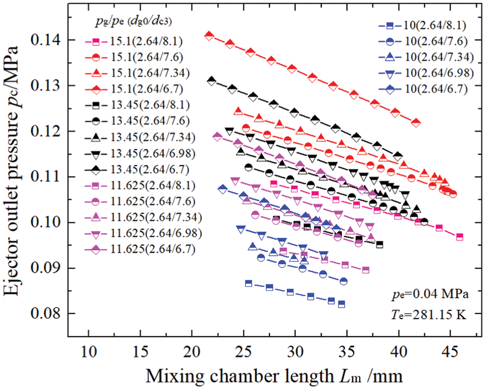
Figure 6: Variations in pc with respect to variations in Lm under different degrees of pg/pe and dg0/dc3

4.2 Variations in Lm

Fig. 7 shows the variations in Lm1 and Lm2 with respect to variations in dg0/dc3 and pg. Figs. 7a and 7b show that a decrease in dg0/dc3 increases Lm1 and decreases Lm2. When dg0/dc3 and pe are constant, Lm1 increases and Lm2 decreases with the decrease of pg. When pg is 0.538 or 0.604 MPa, Lm2 increases and then decreases. When pg is 0.465 or 0.420 MPa, Lm2 decreases and then increases. An increase in dc3 decreases the flow velocity and increases Lm1. When pg increases, the flow rate of the primary flow in Section 2 increases. When dc3 decreases, the intensity of the mixing process increases and Mach number of the fluid in section n Man increases, which decreases Lm1. The regularity of Lm2, which was calculated on the basis of the Fano flow model, is not as obvious as that of Lm1. The main reason is the sensitivity of the friction coefficient model to working conditions. Moreover, when dc3 decreases and pg increases, the flow distance based on the Fano flow increases, which increases Lm2.

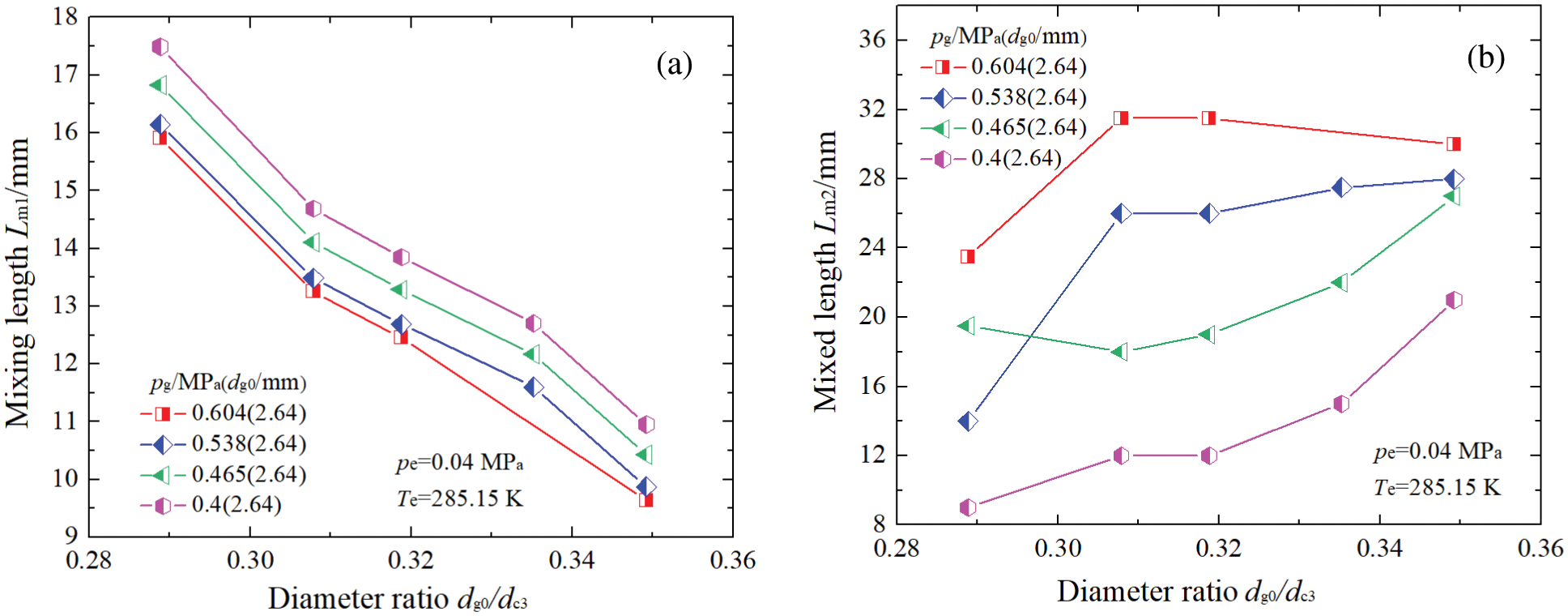
Figure 7: Variations in Lm1 and Lm2 with respect to variations in dg0/d3

4.3 Variations in α and Ld

Fig. 8 shows the variations in α with respect to the variations in dc/dc3 under different degrees of pg/pe and dg0/dc3. When pg/pe is constant, α increases as dc/dc3 decreases. When pg/pe and dc/dc3 are constant, α increases as dg0/dc3 increases. Moreover, when dc/dc3 and dg0/dc3 are constant, α increases as pg/pe increases. Under a range at which dc = 1.8dc3–2.0dc3, α ranges between 6° and 12°. The recommended range of α was reported in references [24] and [25], but there are no significant differences between the calculated using the present model and the recommended in literature. The main reason is the diversity of working conditions such as the working medium and structures of the motive nozzle and mixing chamber.

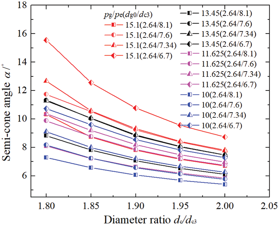
Figure 8: Variations in α with respect to variations in dg0/dc3

Fig. 9 shows the variations in Ld with respect to the variations in dc/dc3 under different degrees of pg/pe and dg0/dc3. As shown in Fig. 9, when pg/pe is constant, Ld increases approximately linearly as dc/dc3 increases. When pg/pe and dc/dc3 are constant, Ld decreases as dg0/dc3 increases. However, when dg0/dc3 and dc/dc3 are constant, Ld increases as pg/pe decreases. Under a range at which dc = 1.8dc3–2.0 dc3, Ld ranges from 9.7 to 34.2 mm.

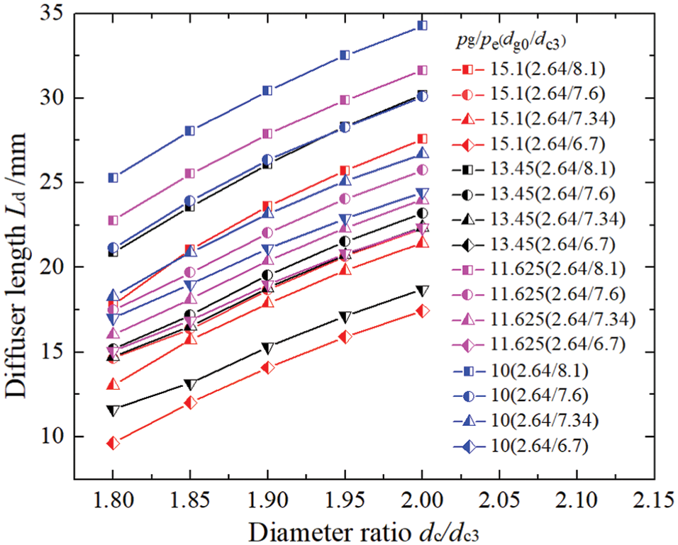
Figure 9: Variations in Ld with respect to variations in dc/dc3

4.4 Variations in Tc and pc with Respect to Variations in Ld

Fig. 10 shows the relationship between Ld and Tc, and Fig. 11 shows the relationship between Ld and pc. When dc/dc3 is constant, an increase in Ld reduces Tc and pc. Especially, Tc and pc decrease significantly when dc3 increases from 6.70 to 6.98 mm. Moreover, when Tc or pc is constant, the larger the dc/dc3, the larger the Ld. This is reasonable because an increase in Ld increases friction loss and decreases Tc and pc.

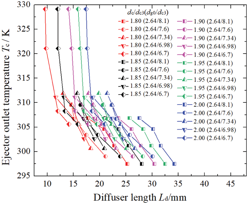
Figure 10: Variations in Tc with respect to variations in Ld

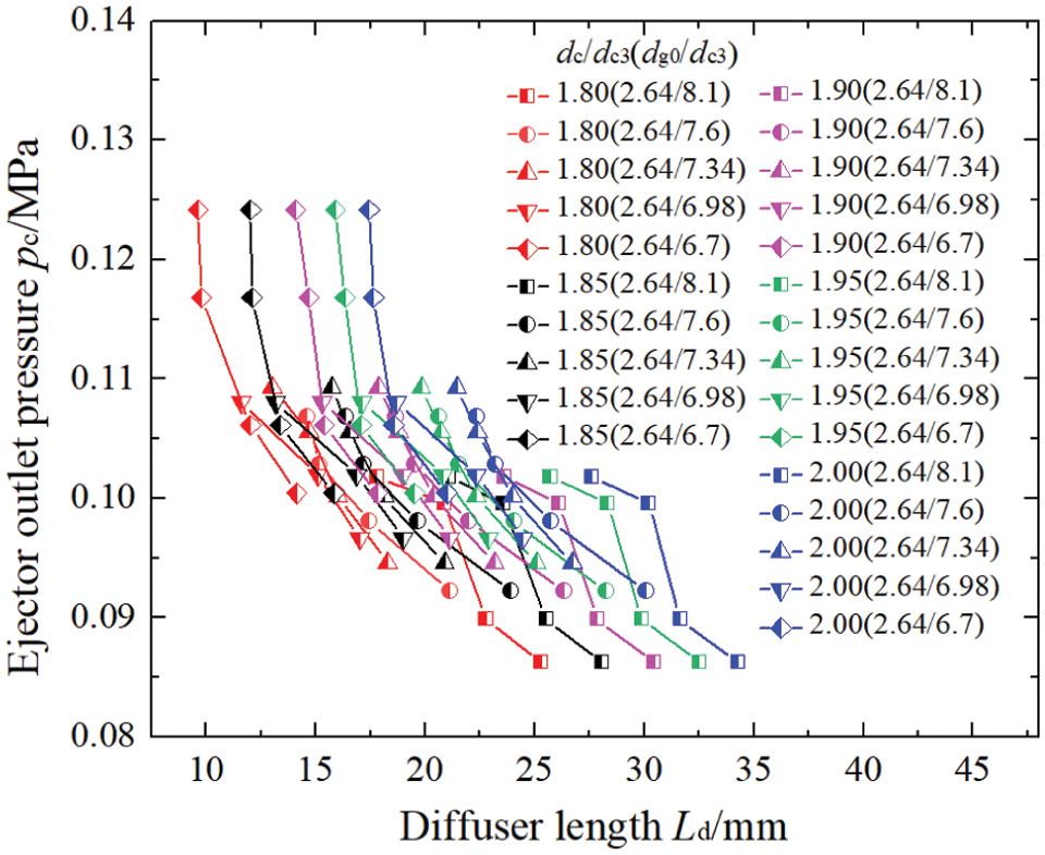
Figure 11: Variations in pc with respect to variations in Ld

4.5 The Distribution of Flow Fields in the Ejector

The two-dimensional CFD model was further developed by using Ansys software to obtain the distribution of flow fields in the ejector. Fig. 12 shows the geometric dimensions of the axisymmetric half-space ejector, which were determined on the basis of the experimental data reported in reference [28] except for the length of the mixing chamber. The corresponding grid chart is shown in Fig. 13. On the basis of the results of the above analysis, we chose Ld to be 32.29 mm and α to be 10°. Details on the operating conditions of the ejector are listed in Table 2.

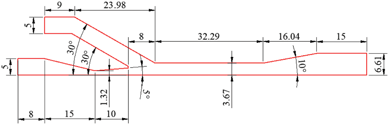
Figure 12: Geometric dimensions of the axisymmetric half-space ejector (length unit: mm)

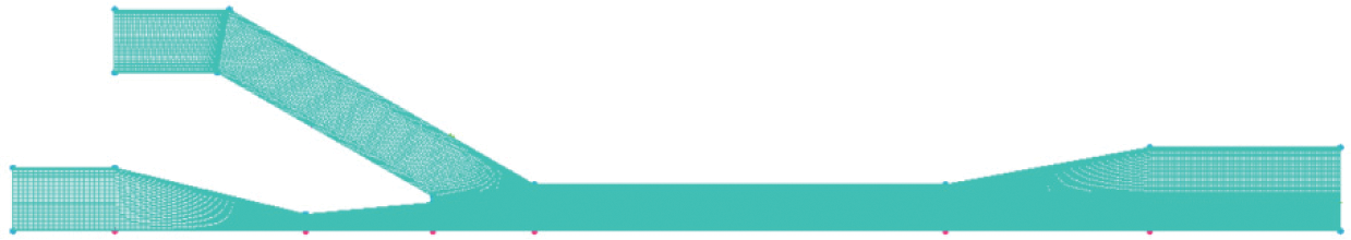
Figure 13: The grid chart of the ejector

Fig. 14 shows the distribution of flow fields in the ejector, including the distribution of pressure, temperature, velocity, Mach number, and streamline of the fluid in the ejector. Fig. 14a shows that pressure reduces and then increases along the axis of the ejector, and there is a shock wave in the mixing chamber. As shown in Fig. 14b, due to entrainment in the suction chamber, a low-pressure region is produced and temperature decreases. In addition, the distribution of the Mach number, which is shown in Fig. 14c, and that of velocity, which is shown in Fig. 14d, indicates that the velocity of the fluid reaches supersonic speed in the nozzle throat, and the Ma of the fluid is close to 1.0. Then, the fluid with supersonic speed leaves the motive nozzle and flows to the location of the shock wave. Fig. 14e shows the fluid streamline in the ejector. The secondary flow enters the suction chamber, and the two streams begin to mix before flowing out of the ejector.

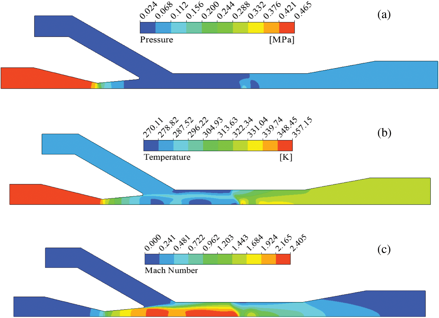
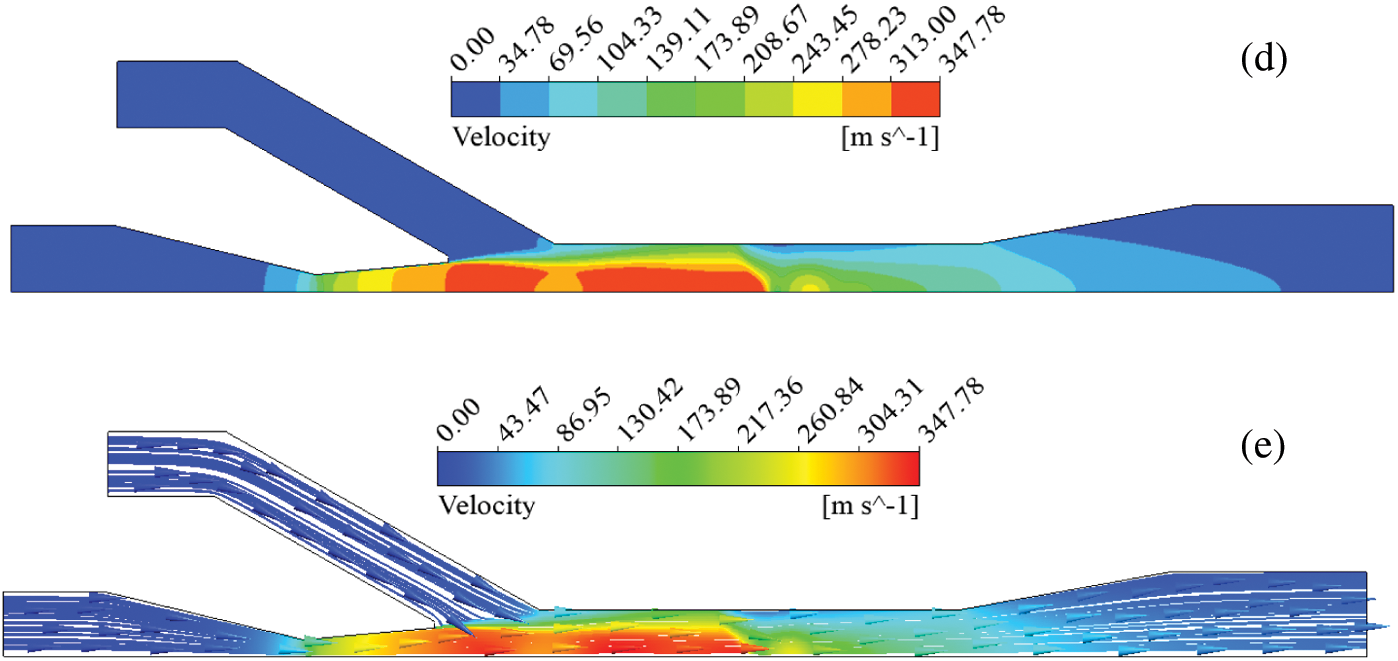
Figure 14: Flow field distributions in the ejector

5  Conclusions

In this paper, an improved model to calculate the mixing chamber length was established on the basis of the Fano flow model, and a method was proposed to optimize the diffuser structure, which considered the frictional resistance and changes in cross-sectional area. To ensure the validity of the model, we compared the theoretical results calculated using the model to experimental data reported in literature. The average error of the calculated entrainment ratio μ was 6.76%, the average error of the calculated outlet temperature of ejector Tc was 0.79%, and the average error of the calculated pc was 6.33%.

Variations in mixing chamber length Lm and diffuser length Ld with respect to variations in Tc and pc were investigated. Variations in mixing section length Lm1 and mixed section length Lm2 with respect to variations in diameter ratio dg0/dc3 were discussed. Relationships among Ld, expansion ratio pg/pe, and diameter ratio dc/dc3 were analyzed. The distribution of flow fields in the ejector was obtained.

An increase in Lm1 decreased Tc and pc. Decreases in pg/pe and dc3 reduced Tc and pc. Furthermore, a decrease in primary flow pressure pg and an increase in mixing chamber diameter dc3 increased Lm1. Lm2 and Lm1 showed an opposite trend.

A decrease in pg/pe and an increase in dc/dc3 reduced the semi-cone angle of the diffuser α. Decreases in Tc and pc increased Ld. Moreover, when Tc or pc was constant, the larger the dc/dc3, the larger the Ld.

In the future, to perform more complicated and flexible computer-aided design (CAD), we will employ Non-Uniform Rational B-Splines (NURBS) to represent the geometry of the ejector. Then, isogeometric analysis [31] will be performed on the basis of the Fano flow model to connect CAD and numerical analysis. By using the control points of NURBS as design variables, we will adopt a gradient-based shape optimization algorithm to automatically search a large design space for the optimal geometry of the ejector. Furthermore, we will investigate the application of the isogeometric boundary element method, which has boundary representation properties, to reduce the dimension of the problem and facilitate the variation in geometry, thus, alleviate the mesh burden associated with iterative shape optimization procedures [32,33].

Funding Statement: This work was supported by the National Natural Science Foundation of China (Grant No. 51806132), Central Guided Local Science and Technology Development Foundation (Grant No. YDZX20201400001939), and Scientific and Technological Innovation of Colleges and Universities of Shanxi Province (Grant No. 201802011).

Conflicts of Interest: The authors declare that they have no conflicts of interest to report regarding the present study.

References

 1.  Lee, J. S., Baek, S. W., Jeong, S. K. (2018). Investigation of the ejector application in the cryogenic joule-thomson refrigeration system. Energy, 165, 269–280. DOI 10.1016/j.energy.2018.09.146. [Google Scholar] [CrossRef]

 2.  Zhang, J., Yin, S. S., Chen, L., Ma, Y. C., Wang, M. J. et al. (2020). A study on the dynamic characteristics of the secondary loop in nuclear power plant. Nuclear Engineering and Technology, 53(5), 1436–1445. DOI 10.1016/j.net.2020.11.014. [Google Scholar] [CrossRef]

 3.  Levchenko, D. O., Artyukhov, A. E., Yurko, I. V. (2017). Maisotsenko cycle applications in multi-stage ejector recycling module for chemical production. Materials Science and Engineering, 233(1), 012024. DOI 10.1088/1757-899X/233/1/012024. [Google Scholar] [CrossRef]

 4.  Bourhan, M. T., Al-Nimr, M. A., Khasawneh, M. A. (2019). A comprehensive review of ejector design, performance, and applications. Applied Energy, 240, 138–172. DOI 10.1016/j.apenergy.2019.01.185. [Google Scholar] [CrossRef]

 5.  Gu, R., Sun, M. B., Li, P. B., Cai, Z., Yao, Y. Z. (2021). A novel experimental method to the internal thrust of rocket-based combined-cycle engine. Applied Thermal Engineering, 196. DOI 10.1016/j.applthermaleng.2021.117245. [Google Scholar] [CrossRef]

 6.  Suryanto, S., Nur, H., Akhmad, T. (2020). The novel vacuum drying using the steam ejector. Drying Technology, 39(7), 905–911. DOI 10.1080/07373937.2020.1728307. [Google Scholar] [CrossRef]

 7.  Salmi, M., Menni, Y., Chamkha, A. J., Ameur, H., Maouedj, R. et al. (2021). CFD-Based simulation and analysis of hydrothermal aspects in solar channel heat exchangers with various designed vortex generators. Computer Modeling in Engineering & Sciences, 126(1), 1–27. DOI 10.32604/cmes.2020.012839. [Google Scholar] [CrossRef]

 8.  Peng, H., Zhang, P. (2018). Numerical simulation of high speed rotating waterjet flow field in a semi enclosed vacuum chamber. Computer Modeling in Engineering & Sciences, 114(1), 59–73. DOI 10.3970/cmes.2018.114.059. [Google Scholar] [CrossRef]

 9.  Wang, C., Wang, L., Zhao, H. X., Do, Z. Y., Ding, Z. Q. (2016). Effects of superheated steam on non-equilibrium condensation in ejector primary motive nozzle. International Journal of Refrigeration, 67, 214–226. DOI 10.1016/j.ijrefrig.2016.02.022. [Google Scholar] [CrossRef]

10. Yang, Y., Zhu, X. W., Yan, Y. Y., Ding, H. B., Wen, C. (2019). Performance of supersonic steam ejectors considering the nonequilibrium condensation phenomenon for efficient energy utilization. Applied Energy, 242, 157–167. DOI 10.1016/j.apenergy.2019.03.023. [Google Scholar] [CrossRef]

11. Wu, Y. F., Zhao, H. X., Zhang, C. Q., Wang, L., Han, J. T. (2018). Optimization analysis of structure parameters of steam ejector based on CFD and orthogonal test. Energy, 151, 79–93. DOI 10.1016/j.energy.2018.03.041. [Google Scholar] [CrossRef]

12. Nakagawa, M., Marasigan, A. R., Matsukawa, T., Kurashina, A. (2011). Experimental investigation on the effect of mixing length on the performance of two-phase ejector for CO2 refrigeration cycle with and without heat exchanger. International Journal of Refrigeration, 34(7), 1604–1613. DOI 10.1016/j.ijrefrig.2010.07.021. [Google Scholar] [CrossRef]

13. Dong, J. M., Hu, Q. Y., Yu, M. Q., Han, Z. T., Cui, W. B. et al. (2020). Numerical investigation on the influence of mixing chamber length on steam ejector performance. Applied Thermal Engineering, 174, 115204DOI 10.1016/j.applthermaleng.2020.115204. [Google Scholar] [CrossRef]

14. Zheng, L. X., Deng, J. Q. (2017). Research on CO2 ejector component efficiencies by experiment measurement and distributed-parameter modeling. Energy Conversion and Management, 142, 244–256. DOI 10.1016/j.enconman.2017.03.017. [Google Scholar] [CrossRef]

15. Avila, R., Han, Z., Atluri, S. N. (2011). A novel MLPG-finite-volume mixed method for analyzing stokesian flows & study of a new vortex mixing flow. Computer Modeling in Engineering & Sciences, 71(4), 363–396. DOI 10.3970/cmes.2011.071.363. [Google Scholar] [CrossRef]

16. Zhu, Y. H., Cai, W. J., Wen, C. Y., Li, Y. Z. (2009). Numerical investigation of geometry parameters for design of high performance ejectors. Applied Thermal Engineering, 29(5–6), 898–905. DOI 10.1016/j.applthermaleng.2008.04.025. [Google Scholar] [CrossRef]

17. Wu, H. Q., Liu, Z. L., Han, B., Li, Y. X. (2014). Numerical investigation of the influences of mixing chamber geometries on steam ejector performance. Desalination, 353, 15–20. DOI 10.1016/j.desal.2014.09.002. [Google Scholar] [CrossRef]

18. Fu, W. N., Liu, Z. L., Li, Y. X., Wu, H. Q., Tang, Y. Z. (2018). Numerical study for the influences of primary steam motive nozzle distance and mixing chamber throat diameter on steam ejector performance. International Journal of Thermal Sciences, 132, 509–516. DOI 10.1016/j.ijthermalsci.2018.06.033. [Google Scholar] [CrossRef]

19. AbdEl-hamid, A. A., Mahmoud, N. H., Hamed, M. H., Hussien, A. A. (2018). Gas-solid flow through the mixing duct and tail section of ejectors: Experimental studies. Powder Technology, 328, 148–155. DOI 10.1016/j.powtec.2018.01.011. [Google Scholar] [CrossRef]

20. Sierra-Pallares, J., del Valle, J. G., Paniagua, J. M., García, J., Bueno, C. M. et al. (2018). Shape optimization of a long-tapered R134a ejector mixing chamber. Energy, 165, 422–438. DOI 10.1016/j.energy.2018.09.057. [Google Scholar] [CrossRef]

21. Chen, H. J., Lu, W., Zhang, G. L. (2015). Method for design and optimization of cylindrical mixing chamber ejector based on real gas properties. Ciesc Journal, 10, 79–85. DOI 10.11949/j.issn.0438-1157.20150150. [Google Scholar] [CrossRef]

22. Ameur, K., Aidoun, Z., Ouzzane, M. (2018). Experimental performances of a two-phase R134a ejector. Experimental Thermal and Fluid Science, 97, 12–20. DOI 10.1016/j.expthermflusci.2018.03.034. [Google Scholar] [CrossRef]

23. Yuan, F., He, D. F., Feng, K., Zhang, M. H., Wang, H. B. (2018). Optimal design and experimental study of ejector for ladle baking. Steel Research International, 89(12), 1800051. DOI 10.1002/srin.201800051. [Google Scholar] [CrossRef]

24. Elbel, S., Hrnjak, P. (2008). Experimental validation of a prototype ejector designed to reduce throttling losses encountered in transcritical R744 system operation. International Journal of Refrigeration, 31(3), 411–422. DOI 10.1016/j.ijrefrig.2007.07.013. [Google Scholar] [CrossRef]

25. Banasiak, K., Hafner, A., Andresen, T. (2012). Experimental and numerical investigation of the influence of the two-phase ejector geometry on the performance of the R744 heat pump. International Journal of Refrigeration, 35(6), 1617–1625. DOI 10.1016/j.ijrefrig.2012.04.012. [Google Scholar] [CrossRef]

26. Yapici, R., Ersoy, H. K. (2005). Performance characteristics of the ejector refrigeration system based on the constant area ejector flow model. Energy Conversion and Management, 46(18–19), 3117–3135. DOI 10.1016/j.enconman.2005.01.010. [Google Scholar] [CrossRef]

27. Pan, J. S., Shan, P. (2011). Fundamentals of gas dynamics, 2011 Revised Edition. Beijing: National Defense Industry Press. [Google Scholar]

28. Huang, B. J., Chang, J. M., Wang, C. P., Petrenko, V. A. (1999). A 1-D analysis of ejector performance. International Journal of Refrigeration, 22(5), 354–364. DOI 10.1016/S0140-7007(99)00004-3. [Google Scholar] [CrossRef]

29. Zhu, Y. H., Cai, W. J., Wen, C. Y., Li, Y. Z. (2007). Shock circle model for ejector performance evaluation. Energy Conversion and Management, 48(9), 2533–2541. DOI 10.1016/j.enconman.2007.03.024. [Google Scholar] [CrossRef]

30. Zuker, R. D., Biblarz, O. (2002). Fundamentals of gas dynamics, 2nd edition. Hoboken: John Wiley & Sons Inc. [Google Scholar]

31. Hughes, T., Cottrell, J., Bazilevs, Y. (2005). Isogeometric analysis: CAD, finite elements, NURBS, exact geometry and mesh refinement. Computer Methods in Applied Mechanics and Engineering, 194(39–41), 4135–4195. DOI 10.1016/j.cma.2004.10.008. [Google Scholar] [CrossRef]

32. Lian, H., Kerfriden, P., Bordas, S. (2016). Implementation of regularized isogeometric boundary element methods for gradient-based shape optimization in two-dimensional linear elasticity. International Journal for Numerical Methods in Engineering, 106(12), 972–1017. DOI 10.1002/nme.5149. [Google Scholar] [CrossRef]

33. Lian, H., Kerfriden, P., Bordas, S. (2017). Shape optimization directly from CAD: An isogeometric boundary element approach using T-splines. Computer Methods in Applied Mechanics and Engineering, 317(4), 1–41. DOI 10.1016/j.cma.2016.11.012. [Google Scholar] [CrossRef]

This work is licensed under a Creative Commons Attribution 4.0 International License, which permits unrestricted use, distribution, and reproduction in any medium, provided the original work is properly cited.