Computer Modeling in Engineering & Sciences

---

DOI: 10.32604/cmes.2022.020350

ARTICLE

Dense-Structured Network Based Bearing Remaining Useful Life Prediction System

Ping-Huan Kuo1,2, Ting-Chung Tseng1, Po-Chien Luan2 and Her-Terng Yau1,2,*

1Department of Mechanical Engineering, National Chung Cheng University, Chiayi, 62102, Taiwan
2Advanced Institute of Manufacturing with High-Tech Innovations (AIM-HI), National Chung Cheng University, Chiayi, 62102, Taiwan
*Corresponding Author: Her-Terng Yau. Email: htyau@ccu.edu.tw
Received: 18 November 2021; Accepted: 11 February 2022

1  Introduction

Many kinds of neural network approaches have been applied in engineering problems [1–3]. Manufacturers and companies need to maintain their competitive advantage by improving the availability, reliability, and safety, reducing the production equipment’s maintenance costs, and keeping them in good working condition. One solution to the problem above is to adopt an appropriate maintenance strategy. In this field, the Condition Based Maintenance (CBM) and Predictive Maintenance (PM) are the most effective since the maintenance is optimized through failure prediction [4]. Unlike traditional corrective maintenance, in which the maintenance is performed only when a failure occurs, the CBM is performed based on the observed or estimated health condition of the equipment [5].

This study is focused on the effects caused by the various forces applied to the bearings. Statistically, bearing failure accounts for approximately 45% of mechanical problems [6]. The wear condition of bearings varies and is influenced by dynamic cutting forces. High-speed machining reduces processing time and thus improves productivity but accelerates the wear of spindle bearings. More attention is required for the maintenance of bearings [7].

The use of a predictive maintenance strategy minimizes the chance of equipment failure. It also prevents more serious damage to the equipment and operators alike. This study is focused on predictive maintenance as well. The proposed bearing Remaining Useful Life (RUL) prediction system aims to reduce the chance of equipment failure.

Failure prediction not only helps improve the availability and reliability of the equipment but also reduces the maintenance costs. Failure prediction aims to predict the time before a failure occurs through the estimation of RUL. The estimated RUL can be used to make sensible decisions based on the future development of the industrial system. Medjaher et al. [8] proposed a data-driven prediction method based on signal processing and regression analysis. The method uses PRONOSTIA, an experimental platform for bearings accelerated degradation tests. Lee et al. [9] proposed a deep learning method named Time Series Multiple Channel Convolutional Neural Network (TSMC-CNN) for bearing RUL prediction. The time series data of bearing operations are divided into multiple channels and fed to the convolutional neural network (Computer Numerical Control, CNN) model. The relationship between distantly separated data points is established. The PRONOSTIA bearing dataset is used to evaluate the performance of the proposed method. A comparison of the evaluation results of the proposed method and other related methods is made. Ren et al. [10] proposed a new roller bearing RUL estimation method based on Sparse Representation theory. The estimated RUL is obtained by analyzing the relationships between all measured data. This RUL estimation is based on the similarity of data of adjacent measurements. As it is known, the RUL estimation for industrial machinery and its components is one of the mainstream technologies in advanced manufacturing, which is essential for improving productivity. Given this situation, Carino et al. [11] proposed a reliable health monitoring method for ball bearings. First of all, the proposed method uses Spearman's rank correlation coefficient to analyze the available temperature data and vibration signals. This step focuses on identifying the most important relationships between features and RUL. The method is reinforced with Support Vector Machine (SVM) so that the RUL is predicted through classification mapping. Chen et al. [12] proposed a method. Traditional fault prediction methods can produce only one predicted result, such as temperature, wear or RUL, at a time. In addition, they are not able to produce highly representative features for dealing with the above-mentioned two tasks simultaneously. They proposed a deep residual network based on multi-task learning. The method is a breakthrough by changing the traditional way of using deep neural networks as black boxes. Two types of diagnostic information are fed into the network, which is helpful in mining the potential links between two tasks of fault diagnosis and generating very representative features. Many studies have been dedicated to developing fast and easy RUL estimation methods on top of accuracy. Akuruyejo et al. [13] proposed a new data-driven approach for bearing RUL estimation. It indicates: “Considering the nonlinear and non-stationary bearing vibration signals, the empirical mode decomposition (EMD) method is used as the pre-processing step for feature extraction. Then, the principal component analysis algorithm (PCA) is used for feature reduction.” Lei et al. [14] proposed a model-based method for RUL prediction of machinery. It indicates: “The method includes two modules, i.e., indicator construction and RUL prediction. In the first module, a new health indicator named weighted minimum quantization error is constructed, which fuses mutual information from multiple features and properly correlates to the degradation processes of machinery. In the second module, model parameters are initialized using the maximum-likelihood estimation (MLE) algorithm and RUL is predicted using a particle filtering-based algorithm.” Electric discharge machining current causes a significant amount of damage to bearings. Different RUL prediction methods must be used to deal with this situation successfully. Singleton et al. [15] indicated: “both experimental and computational approaches for RUL estimation of bearings by taking advantage of the relationship between current discharge events and the vibration signals. A test bed, which induces accelerated aging via applied electrical stress, is introduced to better understand the relationships between bearing currents, vibrations and failures.”

Machine learning is an important field of study as of now. It is commonly used in a variety of applications, such as medical diagnosis [16]. Accurate diagnosis of a disease is crucial because it improves the effectiveness of disease prevention and treatments. In addition, a machine learning model can also be used to analyze the molecular structure of the viruses, which helps us deal with the global spread of COVID-19 [17]. Machine learning can help us predict and prevent natural disasters as well. For example, machine learning can be applied to model droughts [18] and to provide early warning of natural disasters. Machine learning has been used for bearing RUL prediction in recent years as well. Zheng [19] proposed a method to obtain the horizontal vibration signals of a bearing by using a continuous wavelet transform spectrogram and using an exponential degradation mode to predict bearing RUL. Nair et al. [20]. proposed a hybrid model to predict bearing RUL. The perspective of tuning the parameters of the physics-based equations with data from Finite Element Simulations and interpolating for the remaining values gives us a broad look over the correlation between the parameters. In addition, Wang et al. [21]. proposed a bearing RUL prediction method that combines exponential degradation models and Fréchet distance and relatively good prediction performance is achieved. This study uses various neural network architectures to deal with the bearings with different cutting forces. The goal is to develop a model capable of easy and fast bearing condition prediction in different conditions and to offer benefits to the industry.

This paper proposes an integral data processing and neural network architecture that other deep learning neural networks can reference. This study offers a faster yet integral data processing approach. Most of the data used to train the proposed neural network model are matched by the model. This model offers a training method from a wider perspective.

In this study, the acting force on the bearing is a constantly changing factor in the manufacturing process. Since the wear condition is determined by the force applied onto the bearing, the bearing RUL is different in each case. Various types of data are used to train the model proposed in this study, which helps improve the bearing RUL prediction performance under different acting forces. Since this model requires only a small amount of data for training, less time is spent on preparing the training data. The model proposed in this study requires less time in data preparation and achieves faster model training. The same model can accommodate different types of acting forces and thus can be easily used for more bearing RUL predictions.

2  System Architecture

This study uses the National Aeronautics and Space Administration (NASA) dataset for model training. The dataset is composed of machining time, X-axis and Y-axis vibration signals measured by accelerometers, and temperature data. However, the temperature data are missing in some data entries and are not used in this study. Bearing RUL is the output label. Cross-validation is used to evaluate the performance, i.e., prediction accuracy and usefulness, of the model. The model is modified based on whether it matches with data and diagnostic errors. Flow chart of the prediction model as shown in Fig. 1.

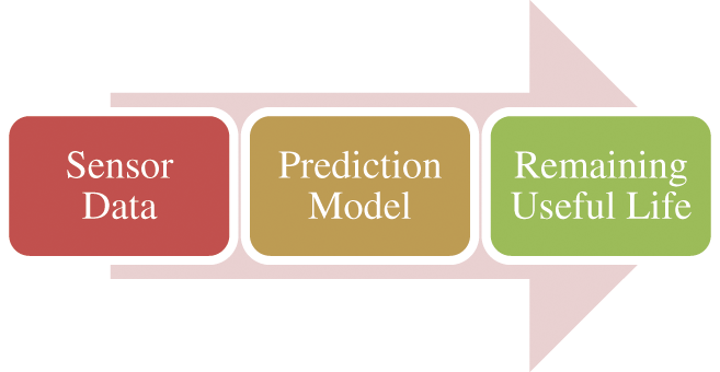
Figure 1: Conceptual representation of prediction model

This study uses NASA Prognostics Center of Excellence-Data Repository, (PCoE) dataset [22,23]. Prognostics Data Repository is a collection of datasets donated by many universities or companies. This study uses the bearing dataset provided by FEMTO-Science & Technologies (FEMTO-ST), Besançon, France. The data come from the test platform, which uses AC Motor to drive the spindle and simulate the rotation of the spindle that causes bearing wear. Accelerometers, force sensors and temperature sensors are used to measure vibration signals, temperature and forces exerted on the bearings. The test platform is shown in Fig. 2.

Figure 2: Conceptual representation of the test platform

The acting force in this paper is defined as the radial force exerted on the bearings. The instantaneous value of acting force is measured. The data of the bearing, the axis that the bearing rotates around and the rotation speed of the torque applied to the bearing are all collected at the frequency of 100 Hz. However, the bearing RUL is defined by the bearing wear, which is determined based on the vibration signals measured by the accelerometers. The bearing vibration signals are measured with two accelerometers positioned perpendicular to each other. One is placed vertically and the other is placed along the horizontal axis. Both accelerometers are placed on the outer ring of the bearing. The sampling rate of the accelerometers is set to 25.6 kHz.

The dataset consists of 17 sets of complete bearing life data. Fig. 3 shows the vibration signals from a part of the bearing data. To simplify the matter, the data in the dataset are divided into three groups depending on the force exerted on the bearings, namely 4000 N, 4200 N and 5000 N. They are shown in Figs. 3–5. The lengths of vibration signals are so different, which poses a huge challenge for training. Data variation and integrity have a great impact on the training process of a neural network and the results. To achieve better results of training, one of the three bearing datasets is chosen as training data and the rest as test data. The goal is to test if the trained model is capable of accurately predicting the bearing RUL. The dataset is divided into groups, as shown in Table 1.

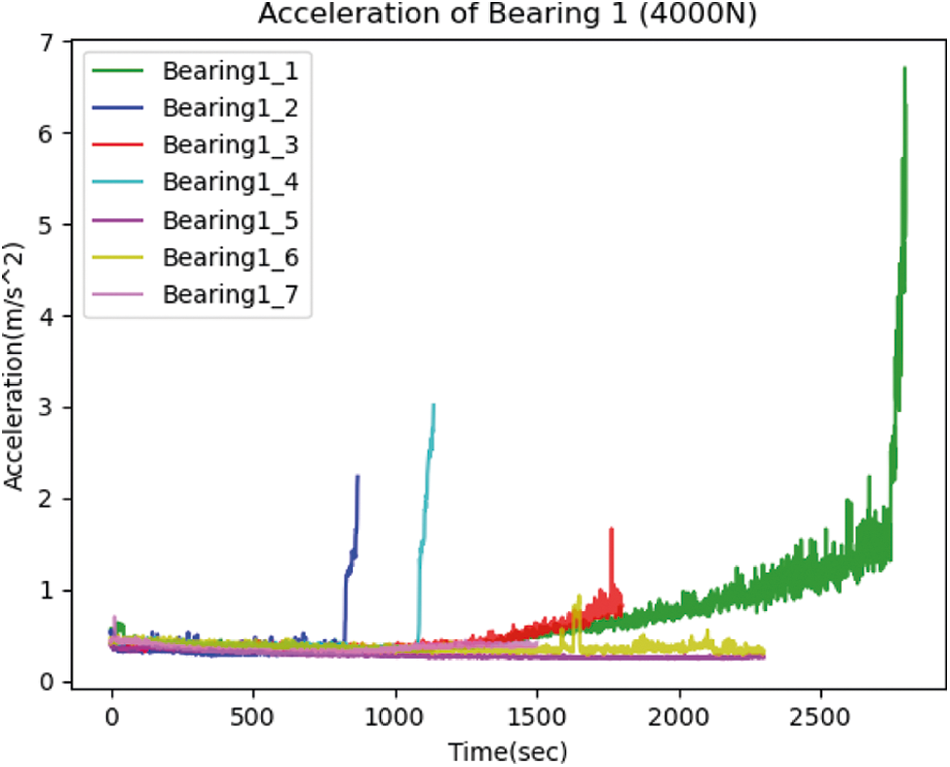
Figure 3: The vibration signals with 4000 N of force acting on the bearing

Figure 4: The vibration signals with 4200 N of force acting on the bearing

Figure 5: The vibration signals with 5000 N of force acting on the bearing

Due to the complicated structure and large size, the sensor data need to be pre-processed. There are at most seven million sensor data entries for one entire bearing life data. The large size of data may have adverse effects on modeling. In addition, the data collected for each bearing are not exactly the same. The bearing data that are too different may cause problems for modeling. A simple pre-processing of sensor data of bearings is hence necessary. The goal is to ensure the data integrity for modeling.

Therefore, the data need to be pre-processed before modeling. Bearing vibration signals are dynamic and complicated. Many approaches for feature extraction for bearing vibration signals have been used [4,24]. Not a single approach has an advantage over the others. This paper introduces three steps for data pre-processing, i.e., data selection and splitting, standard deviation, and normalization.

2.1 Data Selection and Splitting

The most important variable of the data in the dataset is the force exerted on the bearing. However, a clear distinction still exists among the sensor data measured with the same condition of force. The largest difference between bearing RULs with the same variable is as high as 19,310 s, which may lead to deviant behavior of the model. The first 15,000 s of that data of the bearing with greater than 25,000 s of RUL are discarded. Also, the first 10,000 s of that data of the bearing with greater than 20,000 s of RUL are discarded. There are only 1,720 and 3,520 s of sensor data collected from Bearing3_3 and Bearing2_7, respectively. Due to the significant difference in data size, the Bearing2_7 data are not used for RUL prediction model training. The detailed information is shown in Table 2.

2.2 Standard Deviation

The bearing data sizes differ greatly from each other. The bearing RUL prediction is based on the variation trend of vibration signals. In this study, a mean is calculated for every 10 s of data. Two different methods, i.e., Standard Deviation (SD) and mean deviation (Root Mean Square, RMS) [25] are often used for data processing. Mean deviation reflects the averaged difference between tag value and arithmetic mean within an interval. It is best used on normally distributed data. Standard deviation measures the spread of a set of data. The features of vibration signals are represented as the degree of the spread. This study chooses standard deviation other than mean deviation as a data processing method because it produces better model training results. The standard deviation and mean deviation are calculated as shown in Eqs. (1) and (2).

RMS=∑i=1Nxi2N(1)

SD=1N∑i=1N(xi−μ)2(2)

where N denotes the total amount of data; xi denotes the value of i-th item; μ denotes the mean. The feature extraction is performed on every 2,560 sets of vibration signals. The vibration signals are added with other parameters and normalized to form the final training dataset.

2.3 Characteristic Normalization

Feature normalization [26] is a scaling technique in which feature data are rescaled so that they end up falling within a specified range. If the feature data spread over a larger range, the predicted values tend to be higher and the prediction accuracy drops, which can be seen in Table 2. The difference in individual bearing RULs may have influences on the weights. Feature normalization has many advantages, such as making the weights more evenly distributed, avoiding overtraining caused by using the same type of data and improving the bearing RUL prediction accuracy of the model. In this study, the feature data are normalized between 0 and 1. The goal is to make calculating the errors easier. Data normalization is performed as shown below:

xnormalize=x−xminxmax−xmin∈[0,1](3)

where xnormalize denotes the target value and x, xmin, xmax denote original value, minimum value and maximum value of the data, respectively.

3  The Proposed Method

This section introduces the architecture of neural networks. Neural networks are programs designed to mimic the operations of biological neural systems. The goal is to give computers human intelligence so that they are able to behave like humans. In the experiments of this study, a neural network is used as the prediction model. The Multilayer Perceptron (MLP) [27] architecture is shown in Fig. 6 below. The basic architecture is modified and further improved, as shown in Fig. 7. For the architecture proposed in this study, the tensors are connected to more layers. This improvement drastically alleviates the gradient vanishing issue. This architecture is similar to the algorithm in the literature [28]. In this paper, the DenseNets uses skip-connections to complete its computing process [29]. The addition of layers makes shortcut pathways possible for two reasons. This method can improve training stability and alleviate the Yadav et al. [30] indicated: “Vanishing gradient problem. In such methods, each of the neural network’s weights receives an update proportional to the partial derivative of the error function with respect to the current weight in each iteration of training.” This study uses this method to build a Dense-Structured Network (DSN) model. The sensor data are fed into this neural network model and build a bearing RUL prediction model. Cross-validation is also used to evaluate the performance of the neural network as follows. All datasets are categorized into three groups based on the forces exerted in the bearings (i.e., 4000 N, 4200 N, and 5000 N). One dataset from each group is randomly chosen as training data and the rest are used as output parameters. Repeat this process until all combinations of datasets are used, as shown in Fig. 8. The goal of using this approach is to build a neural network model capable of accurate prediction with a limited amount of data. Cross-validation is also used to verify the accuracy of the model. This approach is used to build a neural network model capable of accurate prediction with a limited amount of data. Cross-validation is also used to verify the prediction accuracy of the model. In the first three layers, Rectified Linear Units (ReLU) [31] are used.

Figure 6: Multilayer perceptron architecture

Figure 7: Dense-structured network architecture

Figure 8: Conceptual representation of cross-validation

The DSN model proposed in this study has four fully connected layers in the first half. Each layer is composed of multiple neurons. The effectiveness of training can be improved by adding more neurons. In this study, each of the first three layers contains 50 neurons and the fourth one has 10. After many times of training, this model is found to have the best prediction performance. Each layer has 50, 50, 50 and 10 nodes, respectively. The results are fed into the Sigmoid function as output.

The model proposed in this study uses fully connected layers of neural network to train the model parameters. The goal is to model the complex bearing wear phenomenon through training. However, the gradient vanishing problem often occurs when training with the model that consists of fully connected layers. The weights in the front layers of the neural networks sometimes do not get updated and the weights near the input layer are updated at a very small rate. However, this paper emphasizes that the proposed prediction model can deal with multiple acting forces, which means large variation of data to the input layer. This model takes a shortcut by skipping the neural network layer and using the data to train the next layer in order to avoid the vanishing gradient problem. Therefore, the model proposed in this study is particularly useful in the bearing RUL prediction when there are multiple acting forces. This architecture improves the effectiveness of the model training when a large variation exists in the training data.

The activation function of each layer in the proposed DSN model are listed in the Table 3. Mean square error is chosen as the loss function of DSN to minimize error between prediction and true values. We adopt Adam optimizer as the optimizer due to its self-adaptive characteristic. The training batch size is set to 50, and the total epochs are 500 to guarantee convergence.

Decision Tree (DT) [32] is machine learning algorithm used to solve classification problems. The decision for which node to branch into is made based on the attribute. The decisions are made repeatedly until an outcome is obtained, as shown in Fig. 9. The method is an extended supervised learning algorithm based on the binary branching theory. The rules of the decision trees are obtained through the training process. Decision tree is a quite simple machine learning algorithm. The method is extremely intuitive and is widely used. The model proposed in this paper keeps adding new nodes during the training process until the classification results of the final node contain less than two sample parameters.

Figure 9: Conceptual representation of decision tree

Random Forest, as shown in Fig. 10, is basically a collection of decision trees. A more powerful model is built by integrating multiple learners (i.e., decision trees) and randomly distributed training data. Like a decision tree, Random Forest is a machine learning algorithm suitable for solving classification problems. They share similar decision models for solving regression and classification problems. Random Forest classifies samples by taking a majority vote on the outcomes of a collection of decision trees and solves regression problems by calculating the mean of all decision tree outputs. Therefore, Random Forest is capable of analyzing nonlinear data effectively and outperforms the multiple linear regression method. No assumption of the type of a given model is needed. Compared with decision trees, Random Forest has better prediction accuracy and prevents overfitting. More nodes are added continuously to the model during the training process until the classification result of the final node has fewer than two sample parameters. In general, it achieves a better regression effect than the regression tree does.

Figure 10: Conceptual representation of random forest

Support Vector Regression (SVR) is an important branch of application of Support Vector Machine (SVM), as shown in Fig. 11. SVM model aims to construct a hyperplane that distinctly classifies the data points for prediction or classification purposes. The model in this paper uses SVR, which is conceptually similar to SVM. It is capable of solving continuous regression prediction problems by minimizing the distances between data points to the regression line. This model has outstanding performance in classifying nonlinear data and images. SVR gains its robustness by adopting ε-insensitive function, penalty factor C and variables ξi,ξi∗. It is often used to solve nonlinear regression prediction and time series prediction problems. The prediction parameter C in this paper is set to 5. The higher the penalty factor, the bigger the penalty from incorrect classification, and vice versa. Radial Basis Function (RBF) kernel is a popular kernel function used in various kernelized learning algorithms. ϵ is 0.1.

Figure 11: Conceptual representation of support vector machine

4  The Experimental Results

In this study, the results from different algorithms are verified with the Cross-validation method. Cross-validation is a statistical verification method used to evaluate the prediction performance of a model. The performance and accuracy of a model are evaluated by the use of mathematical equations. The validation method uses the relationships between predicted values and actual values to assess the predicted errors. In this study, three indicators are used to evaluate the model's prediction accuracy and matching ability.

4.1 Performance Indicators

Mean Absolute Error (MAE) is the ratio of predicted value to the actual value, which is calculated as follows;

MAE=∑i=1n|yi−y^i|n(4)

where n denotes the total amount of data; yi denotes the actual remaining life; y^i denotes the actual remaining life. The reason for using MAE as the indicator of prediction performance is to find the difference between actual data and predicted data and compare them. The evaluation is performed on each set of data.

As shown below, root-mean-square error (RMSE) is mainly used to test the variation between actual and predicted values.

RMSE=1n∑i=1n(yi−y^i)2(5)

In (5), n denotes the total amount of data; yi denotes actual remaining life; y^i denotes predicted remaining life. This method is mainly used to evaluate the model’s prediction performance and represent it in numerical form.

Coefficient of determination (R2 Score) is a statistical measurement that represents the proportion of the variation in the dependent variable. It is a convenient, intuitive measurement used to test the goodness of fit between actual and model-predicted values.

R2=1−∑in(yi−y^i)2∑in(yi−y¯)2(6)

where n denotes the total amount of data; yi denotes actual remaining life; y^i denotes predicted remaining life; y¯ denotes the mean of remaining life. The goal of this method is to evaluate how well-fitting a regression model is.

4.2 Prediction Results

The experiment results show that the DSN machine learning model proposed in this paper achieves the performance of MAE of 252.98, RMSE of 410 and R2 Score of 0.99, as shown in Fig. 12. The largest difference of MAEs is as high as 1297.91. Compared with other machine learning methods, such as support vector machine (SVM), Random Forest (RF), Decision Tree (DT), Adaptive boosting learning (Adaboost) and Multilayer perceptron (MLP), the model has better prediction capabilities, as shown in Figs. 13–15. The figures show that, compared with other models, DSN prediction results have the bluest dots (i.e., low prediction error) and the least orange dots (i.e., large prediction error). SVR is the model with the second-best prediction results. The prediction errors of the models are shown in Table 4.

Figure 12: DSN prediction results: (a) comparison of actual and predicted values, (b) residual plot

Figure 13: DT prediction results: (a) comparison of actual and predicted values, (b) residual plot

Figure 14: RF prediction results: (a) comparison of actual and predicted values, (b) residual plot

Figure 15: SVR prediction results: (a) comparison of actual and predicted values, (b) residual plot

In this study, a comparison is made between the models based on Decision Tree, Random Forest and Support Vector Regression. These algorithms are not new but still commonly used. They are relative iconic algorithms in the field of machine learning, so that the comparison results are credible.

The experiment results show that the DT model delivers relatively fairly good prediction performance in the early stage. However, it produces high prediction discrepancies and even makes erroneous predictions occasionally in the middle stage of RUL. Compared to the DT model, the RF model delivers similar prediction performance. Both perform better in the early stage of RUL. However, the prediction accuracy drops in certain cases, in which the predicted RUL cannot be obtained. The results show that the SVR model is not suitable for training in this study. Although the DSN training model proposed in this study produces a certain degree of RUL prediction discrepancies in a couple of cases, it, of all models, delivers the best prediction results. The curve of predicted values has the best match with actual values. Therefore, it is known that the DSN prediction model is very suitable for bearing RUL prediction.

In this paper, a comparison of the training time of several algorithms is also made. It takes less than 0.5 s to train the RF model, and about 0.005 s to train the DT and SVR models. The DSN model proposed in this study requires about 3.5 s for training. The model proposed in this study requires a longer time for training but achieves much higher training accuracy than other algorithms. This study aims to develop a machine learning model that can be used on smaller amounts but various types of data and still achieves better bearing RUL prediction accuracy in different conditions.

5  Conclusion

In this study, the bearing vibration signals and RUL data are pre-processed. Then the DSN neural network model proposed in this study is used to predict the bearing RUL. A training method different from a traditional MLP is used this time to solve the gradient vanishing problem, improve the training stability and increase the robustness of the neural network model. A comparison is also made with the aforementioned neural network models to demonstrate that the model matches this dataset. Although built with a small amount of data, the model proposed in this study still matches most of the other datasets. The model is built fast and achieves the goal of high accuracy of predicting bearing RUL. Subsequent actions can be determined immediately and taken based on the prediction results to ensure the safety of machinery and humans and further improve production efficiency and safety.

Funding Statement: This work was supported by the Ministry of Science and Technology, Taiwan, under Grant MOST 110-2218-E-194-010.

Conflicts of Interest: The authors declare that they have no conflicts of interest to report regarding the present study.

References

1. Fallah, M., & Nozari, H. (2021). Neutrosophic mathematical programming for optimization of multi-objective sustainable biomass supply chain network design. Computer Modeling in Engineering & Sciences, 129(2), 927-951. [Google Scholar] [CrossRef]
2. Yu, L., Qin, Z., Ding, Y., & Qin, Z. (2021). MIA-UNet: Multi-scale iterative aggregation U-network for retinal vessel segmentation. Computer Modeling in Engineering & Sciences, 129(2), 805-828. [Google Scholar] [CrossRef]
3. Zuo, F., Jia, M., Wen, G., Zhang, H., & Liu, P. (2021). Reliability modeling and evaluation of complex multi-state system based on Bayesian networks considering fuzzy dynamic of faults. Computer Modeling in Engineering & Sciences, 129(2), 993-1012. [Google Scholar] [CrossRef]
4. Jardine, A. K., Lin, D., & Banjevic, D. (2006). A review on machinery diagnostics and prognostics implementing condition-based maintenance. Mechanical Systems and Signal Processing, 20(7), 1483-1510. [Google Scholar] [CrossRef]
5. Gao, J., & Altintas, Y. (2019). Development of a three-degree-of-freedom ultrasonic vibration tool holder for milling and drilling. IEEE/ASME Transactions on Mechatronics, 24(3), 1238-1247. [Google Scholar] [CrossRef]
6. Nandi, S., Toliyat, H. A., & Li, X. (2005). Condition monitoring and fault diagnosis of electrical motors-A review. IEEE Transactions on Energy Conversion, 20(4), 719-729. [Google Scholar] [CrossRef]
7. Auchet, S., Chevrier, P., Lacour, M., & Lipinski, P. (2004). A new method of cutting force measurement based on command voltages of active electro-magnetic bearings. International Journal of Machine Tools and Manufacture, 44(14), 1441-1449. [Google Scholar] [CrossRef]
8. Medjaher, K., Zerhouni, N., Baklouti, J. (2013). Data-driven prognostics based on health indicator construction: Application to PRONOSTIA's data. 2013 European Control Conference (ECC), pp. 1451–1456. Piscataway, IEEE. DOI 10.23919/ECC.2013.6669223. [CrossRef]
9. Lee, J. E., Jiang, J. R. (2019). Time series multi-channel convolutional neural network for bearing remaining useful life estimation. 2019 IEEE Eurasia Conference on IoT, Communication and Engineering (ECICE), pp. 408–410. Piscataway, IEEE. DOI 10.1109/ECICE47484.2019.8942782. [CrossRef]
10. Ren, L., Lv, W. (2016). Remaining useful life estimation of rolling bearings based on sparse representation. 2016 7th International Conference on Mechanical and Aerospace Engineering (ICMAE), pp. 209–213. Piscataway, IEEE. DOI 10.1109/ICMAE.2016.7549536. [CrossRef]
11. Carino, J. A., Zurita, D., Delgado, M., Ortega, J. A., Romero-Troncoso, R. J. (2015). Remaining useful life estimation of ball bearings by means of monotonic score calibration. 2015 IEEE International Conference on Industrial Technology (ICIT), pp. 1752–1758. Piscataway, IEEE. DOI 10.1109/ICIT.2015.7125351. [CrossRef]
12. Chen, L., Xu, G., Tao, T., & Wu, Q. (2020). Deep residual network for identifying bearing fault location and fault severity concurrently. IEEE Access, 8, 168026-168035. [Google Scholar] [CrossRef]
13. Akuruyejo, M., Kowontan, S., Ali, J. B. (2017). A data-driven approach based health indicator for remaining useful life estimation of bearings. 18th International Conference on Sciences and Techniques of Automatic Control and Computer Engineering (STA), pp. 284–289. Piscataway, IEEE. DOI 10.1109/STA.2017.8314889. [CrossRef]
14. Lei, Y., Li, N., Gontarz, S., Lin, J., & Radkowski, S. (2016). A model-based method for remaining useful life prediction of machinery. IEEE Transactions on Reliability, 65(3), 1314-1326. [Google Scholar] [CrossRef]
15. Singleton, R. K., Strangas, E. G., & Aviyente, S. (2016). The use of bearing currents and vibrations in lifetime estimation of bearings. IEEE Transactions on Industrial Informatics, 13(3), 1301-1309. [Google Scholar] [CrossRef]
16. Kumar, G., & Alqahtani, H. (2022). Deep learning-based cancer detection-recent developments, trend and challenges. Computer Modeling in Engineering & Sciences, 130(3), 1271-1307. [Google Scholar] [CrossRef]
17. Gong, L. J., Zhang, X. X., Zhang, L., & Gao, Z. H. (2021). Predicting genotype information related to COVID-19 for molecular mechanism based on computational methods. Computer Modeling in Engineering & Sciences, 129(1), 31-45. [Google Scholar] [CrossRef]
18. Sundararajan, K., Garg, L., Srinivasan, K., Bashir, A. K., & Kaliappan, J. (2021). A contemporary review on drought modeling using machine learning approaches. Computer Modeling in Engineering and Sciences, 128(2), 447-487. [Google Scholar] [CrossRef]
19. Zheng, Y. (2019). Predicting remaining useful life using continuous wavelet transform integrated discrete teager energy operator with degradation model. 2019 IEEE 5th International Conference on Computer and Communications (ICCC), pp. 240–244. Piscataway, IEEE. DOI 10.1109/ICCC47050.2019.9064232. [CrossRef]
20. Nair, S., Verma, T., Khatri, R. (2019). A hybrid model to predict remaining useful life for a ball bearing. 2019 IEEE Symposium Series on Computational Intelligence (SSCI), pp. 2119–2123. Piscataway, IEEE. DOI 10.1109/SSCI44817.2019.9002688. [CrossRef]
21. Wang, B., Lei, Y., Li, N., & Li, N. (2018). A hybrid prognostics approach for estimating remaining useful life of rolling element bearings. IEEE Transactions on Reliability, 69(1), 401-412. [Google Scholar] [CrossRef]
22. Prognostics Center of Excellence (2021). PCoE: Prognostic data repository. https://ti.arc.nasa.gov/tech/dash/groups/pcoe/prognostic-data-repository/.
23. FEMTO Bearing Data Set (2021). Prognostic data repository. http://ti.arc.nasa.gov/project/prognostic-data-repository.
24. Wang, Y., Tang, B., Qin, Y., & Huang, T. (2019). Rolling bearing fault detection of civil aircraft engine based on adaptive estimation of instantaneous angular speed. IEEE Transactions on Industrial Informatics, 16(7), 4938-4948. [Google Scholar] [CrossRef]
25. Seryasat, O. R., Honarvar, F., Rahmani, A. (2010). Multi-fault diagnosis of ball bearing using FFT, wavelet energy entropy mean and root mean square (RMS). 2010 IEEE International Conference on Systems, Man and Cybernetics, pp. 4295–4299. Piscataway, IEEE. DOI 10.1109/ICSMC.2010.5642389. [CrossRef]
26. Kolarik, M., Burget, R., Riha, K. (2020). Comparing normalization methods for limited batch size segmentation neural networks. 2020 43rd International Conference on Telecommunications and Signal Processing (TSP), pp. 677–680. Piscataway, IEEE. DOI 10.1109/TSP49548.2020.9163397. [CrossRef]
27. Liao, T. W. (1996). Modelling process mean and variation with MLP neural networks. International Journal of Machine Tools and Manufacture, 36(12), 1307-1319. [Google Scholar] [CrossRef]
28. He, K., Zhang, X., Ren, S., Sun, J. (2016). Deep residual learning for image recognition. Proceedings of the IEEE Conference on Computer Vision and Pattern recognition, pp. 770–778. Piscataway, IEEE. DOI 10.1109/CVPR.2016.90. [CrossRef]
29. Huang, G., Liu, Z., van der Maaten, L., Weinberger, K. Q. (2017). Densely connected convolutional networks. Proceedings of the IEEE Conference on Computer Vision and Pattern Recognition, pp. 4700–4708. Piscataway, IEEE. DOI 10.1109/CVPR.2017.243. [CrossRef]
30. Yadav, O., Passi, K., Jain, C. K. (2018). Using deep learning to classify X-ray images of potential tuberculosis patients. IEEE International Conference on Bioinformatics and Biomedicine (BIBM), pp. 2368–2375. Piscataway, IEEE.
31. Maas, A. L., Hannun, A. Y., Ng, A. Y. (2013). Rectifier nonlinearities improve neural network acoustic models. Proceedings of the 30th International Conference on Machine Learning, vol. 30, pp. 1. Atlanta, Georgia, USA.
32. Patil, S., Kulkarni, U. (2019). Accuracy prediction for distributed decision tree using machine learning approach. 2019 3rd International Conference on Trends in Electronics and Informatics (ICOEI), pp. 1365–1371. Piscataway, IEEE. DOI 10.1109/icoei.2019.8862580. [CrossRef]

Appendix

The comparison of prediction results of bearing remaining life using various algorithms is shown in Fig. A1, where the green line represents the prediction results of DSN. The green line matches the red line (i.e., actual values) better. The model always has higher prediction accuracy in different conditions of acting forces and bearing RULs. Of all algorithms, DSN has the best performance based on R2 score. Therefore, DSN is more efficient in predicting the bearing RUL. Most of the prediction results are omitted because of space limitations. Only the RUL prediction results with the training data that combine Bearing1_1, Bearing2_1 and Bearing3_1 data (the rest is test data) are included.

Figure A1: Prediction results of bearing remaining life using various algorithms

This work is licensed under a Creative Commons Attribution 4.0 International License, which permits unrestricted use, distribution, and reproduction in any medium, provided the original work is properly cited.