Computer Modeling in Engineering & Sciences

---

DOI: 10.32604/cmes.2022.020781

ARTICLE

An Efficient Computational Method for Differential Equations of Fractional Type

Mustafa Turkyilmazoglu1,2,*

1Department of Mathematics, Hacettepe University, Ankara, 06532, Turkey
2Department of Medical Research, China Medical University Hospital, China Medical University, Taichung, 40447, Taiwan
*Corresponding Author: Mustafa Turkyilmazoglu. Email: turkyilm@hacettepe.edu.tr
Received: 11 December 2021; Accepted: 22 February 2022

1  Introduction

Fractional differential equations play a significant role in the recent literature in modeling many physical and chemical problems, whose limiting cases of integer-order derivatives are well-studied equations which are transformed into the fractional-order derivatives via certain definitions, such as the Riesz fractional derivative, the Caputo fractional derivative and the Riemann-Liouville fractional integral [1], among many others. The current research is also concerned with the ordinary and partial differential equations of fractional order by means of the approximate series solutions through the Adomian decomposition method accounting for a modified framework.

New trend in the recent literature is to generalize the standard mathematical models to incorporate fractional derivative in place of the integer-valued derivative in time and space. This is necessary to explain various physical phenomena in view of experimental evidences. Much effort was spent to derive and analyze certain realistic models in this respect. From physical point of view, for instance, the time-fractional diffusion equation was solved in [2] by means of the rational approximation of the Mittag-Leffler function. Some oscillation results were given in [3] regarding the fractional-order delay differential equations. Su [4] presented mass-time fractional partial differential equations for shrinking soils. A cancer tumor model with the help of fractional diffusion equation was given in the article [5]. The Navier-Stokes equations involving time fractional differential operator were analyzed in the publication [6]. Fractional Schrödinger equations with bounded potentials were analyzed in the article [7]. Recent applications of newly defined fractional derivatives can be found in [8].

Due to the importance of the fractional differential equations in practical applications, some of which were as mathematically analyzed from the aforementioned bibliography, new computational efforts are needed, since traditional methods may not be suitable in fractional domains. Among several suggested techniques in this direction, we mention the Adomian decomposition method [9–11], the variational iteration method [12], the homotopy analysis method [13,14], and the predictor-corrector methods [15]. More plausible methods developed for the fractional equations based on several variations of finite element and finite difference treatments can be found in [16]. Several numerical methods, including the implicit quadrature, the predictor-corrector, the approximate Mittag-Leffler, the collocation, and the finite differences were compared and discussed in [17] in order for revealing their relative merits in solving the ordinary fractional differential equations, and the recommendation was in favor of the predictor-corrector method. Exponential convergence of the collocation method based on the Mn¨z polynomials was reported in [18]. Fractional order logistic equations were treated by a novel iterative scheme in [19]. The accuracy of the reproducing kernel method for solving fractional order Lane-Emden differential equations was explored in [20] and it was argued that the accuracy was better than that of the collocation approach. The goal of [21] was to construct and efficient fractional finite difference method for linear fractional differential equations of special fractional order. Daraghmeh et al. [22] illustrated that the matrix approach method is better as compared with the homotopy perturbation method. Alchikh et al. [23] introduced a Laplace decomposition method to implement numerical solutions of nonlinear fractional ray equations in optics. Fuzzy fractional differential equations in one or higher dimensions were thoroughly integrated with Spectral collocation method based on Chebyshev polynomials in [24–26]. The time-fractional advection-reaction-diffusion equation was approximated numerically by means of Mittag-Leffler kernel in [27]. The non-singular fractional derivative approach was used in [28] to numerically simulate a mosquito-borne virus. More recent attempts on solutions of fractional order differential equations with various developed methods can be found in the publications [29 –36].

The motivation here is to introduce an accurate and user friendly version of the Adomian Decomposition Technique to particularly approximate the solutions of fractional ordinary and partial differential equations. For this purpose, the classical Adomian decomposition method is modified to incorporate a functional term involving both variable and a parameter. A similar concept was also adopted in the reference [37] from a different perspective without specifying the minimal error. To identify the optimized embedded parameter value, the L2 residual is later employed in the current research. The selected problems from the open literature prove that the offered ADM is superior to the classical ADM and emphasize the accuracy of the proposed version of the Adomian Decomposition Technique as compared to some recently developed numerical means of solving the fractional differential equations.

2  Mathematical Preliminaries

2.1 Fractional Calculus

The traditional Riemann-Liouville’s fractional integral operator and the Caputo’s fractional derivative are used in the following analysis, whose definitions are shortly given below.

Definition 1. The fractional integral operator of order α in the Riemann-Liouville sense, for a function f in the space L1 is defined by

(Iαf)(t)=1Γ(α)∫0t(t−τ)α−1f(τ)dτ,t>0,α>0, (1)

in which Γ stands for the standard Gamma function in Eq. (1).

Definition 2. The fractional derivative in the Caputo sense, for a function f whose nth derivative belongs to L1 is defined by

Dα(f(t))=(In−αDnf)(t)=1Γ(n−α)∫0t(t−τ)n−α−1f(n)(τ)dτ,t>0, (2)

where n−1<α≤n, n∈N in Eq. (2).

2.2 Description of the ADM Method

To briefly outline the Adomian decomposition method, we consider the operational equation

Lu+Nu=f, (3)

where L is an easily invertible linear operator of integer or fractional order such as Caputo’s derivative D(α) in Eq. (2), N is an analytic nonlinear operator, u and f are sufficiently well-behaved functions depending on space variable x and time variable t. We note that Eq. (3) is complemented with suitable initial and boundary constraints depending on the physical problem. To find the unknown u, Eq. (3) is inverted via L−1 (in the sense of Riemann-Liouville operator I(α) in case of fractional order) to yield

u=g+L−1f−L−1Nu, (4)

where g in Eq. (4) is as a result of integration to be determined from the supplemented initial and boundary conditions.

Adomian decomposition method is based on the formulations of the solution and the nonlinearity as

u=∑n=0∞un,Nu=∑n=0∞An, (5)

where An’s in Eq. (5) are the well-documented classical Adomian polynomials [38], obtained from

An=1n![dndλn∑i=0∞λiui]λ=0.

An iterative formula is then obtained by substituting Eq. (5) into Eq. (4) in the format

u0=g+L−1f,un+1=−L−1An,n≥0,(6)

which can be used to approximate the solution to Eq. (3) iteratively up to any level of approximation M

uM=∑n=0Mun. (7)

2.3 Convergence of the ADM Method and Error Bound

In the general case without fractional-order derivative, the ADM technique in Eq. (6) is known to converge to generate an accurate approximate solution Eq. (7), see for instance the article [39]. In the case involving fractional order differentiations, we provide the following Lemma whose proof can be found in the recent publication [15]:

Lemma 1. If the approximation u0 is bounded in the sense of sup absolute value norm, the series in Eq. (7) converges in the limit M→∞ producing exact solution to Eq. (3) given by Eq. (8)

u=∑n=0∞un. (8)

Lemma 2. The error with respect to the maximum absolute truncation of the ADM method is given by

||u−uM||≤rM1−r||u0||, (9)

where 0 < r < 1.

Proof. Subtracting the sequence of partial sums of ADM series solution in Eq. (7) from the full solution u of Eq. (3) and taking into account the boundedness of u0, we obtain Eq. (9)

||u−uM||≤rM1−r||u0||, (10)

refer to [15] for more details regarding Eq. (10). This completes the proof.

2.4 Convergence Acceleration of the ADM Method

In order to accelerate the convergence property of the usual iterative ADM scheme Eq. (6), we propose a modified version by embedding a functional term F(x, t, h) possessing a convergence accelerating parameter h and decomposing Eq. (6) in the form

u0=g+L−1f−F(x,t,h),u1=F(x,t,h)−L−1A0,un+1=−L−1An,n≥1. (11)

Introducing a functional embedding into the classical ADM inEq. (11) was already shown to boost the convergence in [11]. Therefore, in the subsequent examples, the traditional ADM is substituted by the modified ADMEq. (11), which cover the traditional ADM in the absence of embedding function F.

Remark 1. As compared to the traditional ADM given in the previous section, the above presented ADM is more advantageous, since u0 involving an extra term is more controllable and also the parameter r depending on the convergence parameter h can be made adequately small by proper choices.

We note that F(x, t, h) should be an integrable function in terms of either x or t (or both in the case of a partial differential equation), up to an order of n. In this manner, the approximate solution Eq. (7) will be a function of h whose optimum value for the fastest convergence towards the solution Eq. (8) can be assured by means of minimizing the global error from the subsequent residual at the truncation level M by means of

Res(h)=(∫C(Lu+Nu−f)2dA)1/2, (12)

where D is the domain of physical interest with the area element dA and the integration is performed in the space L2.

3  Numerical Experiments

We apply the accelerated ADM method introduced in Eqs. (11) and (12) to several ordinary and partial differential equations of fractional order in this section. Whenever the exact solution ue is known, the pointwise error at the approximation order M having the approximate solution uM is defined via Eq. (13)

|ue−uM|. (13)

3.1 Ordinary Fractional Differential Equations

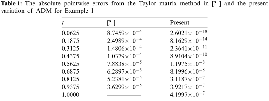
Example 1. To demonstrate the practical applicability of the proposed variation of ADM, we initially take into account the following one-third order fractional differential equation as studied recently in [29] by means of a matrix formulation based on Taylor polynomials

u(1/3)+t1/3u=32Γ(2/3)t2/3+t4/3,u(0)=0,0≤t≤1. (14)

As given in [29], exact solution to Eq. (14) is simply ue(t) = t. Our functional embedding into ADM inEq. (11) for the current problem is represented by the iteration procedure

u0=I(1/3)(32Γ(2/3)t2/3+t4/3)−ht2,u1=−I(1/3)(u0(t))+ht2,un+1=−I(1/3)(un(t)),n≥1. (15)

In Figs. 1a and 1b, the corresponding squared residual error from Eq. (12) as well as the pointwise absolute errors from Eq. (13) are depicted. The classical ADM with h = 0 yields a residual error Res=3.9×10−5. However, the functional embedding ht2 in Eq. (15) gives rise to a much improved residual error Res=5.3×10−7 with the optimal h computed as 1.0409 from the present ADM scheme, see also Fig. 1. Table 1 tabulates the pointwise absolute errors at selected points evaluated from this optimum h, which also includes the pointwise errors from the technique in [29] calculated the same number of Taylor polynomials. It is realized from a direct comparison that the proposed method here works perfectly for the whole physical domain of the considered one-third order fractional differential equation Eq. (14), with a much higher accuracy than the matrix method in [29].

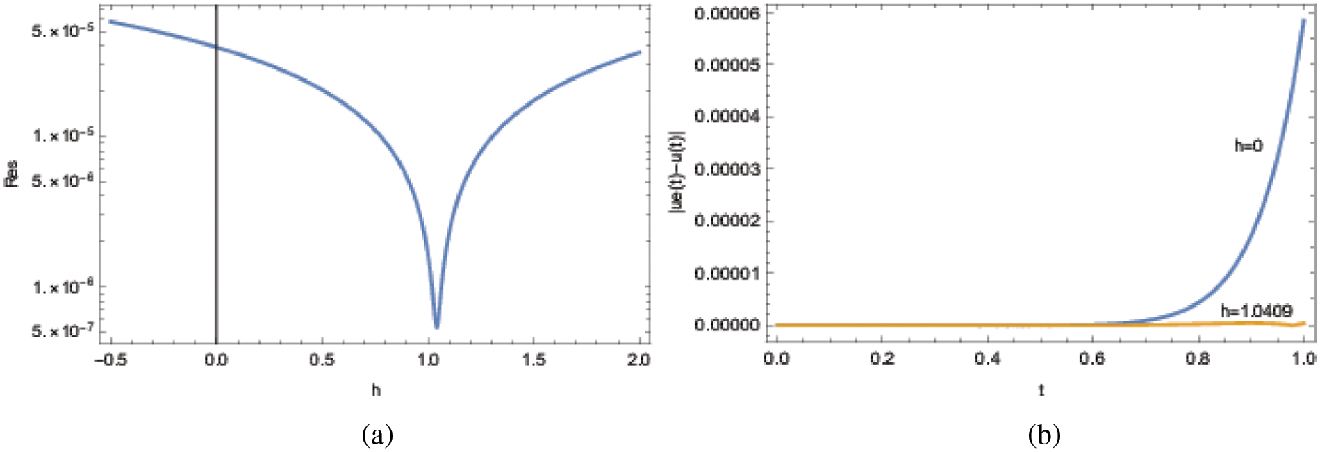
Figure 1: ADM solutions for Example 1 at the approximation level 15. (a) Residual error and (b) pointwise errors

For future reference, the approximate analytical solution from the 15th order modified ADM method used to generate the above results is given by the formula in Eq. (16):

u(t)=t(1−1.11022×10−16t2/3−2.22045×10−16t4/3+1.11022×10−16t5/3+1.11022×10−16t7/3+2.498×10−16t8/3+5.55112×10−17t10/3−1.66533×10−16t11/3−4.16334×10−17t4+5.55112×10−17t13/3−1.38778×10−17t14/3+1.38778×10−17t5−3.46945×10−18t16/3−3.46945×10−18t17/3+1.73472×10−18t6+6.93889×10−18t19/3+1.73472×10−17t20/3+3.46945×10−18t7−3.90313×10−18t22/3−1.73472×10−18t23/3+2.1684×10−19t8+1.30104×10−18t25/3−9.75782×10−19t26/3−7.58942×10−19t9+3.25261×10−19t28/3+4.33681×10−19t29/3−1.0842×10−19t10+4.06576×10−19t31/3−0.0000584367t32/3+0.0000588567t11) (16)

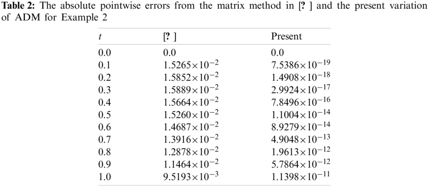
Example 2. The feasibility of proposed ADM for a high-order (α=1.9) fractional differential is next measured by application to the test problem (refer to [17,22])

u(α)+u=2Γ(3−α)t2−α+t2,u(0)=u′(0)=0,0≤t≤1. (17)

The exact solution to Eq. (17) can be worked out as ue(t) = t2. As for the ADMEq. (11) with functional embedding, it is given by

u0=I(α)(2Γ(3−α)t2−α+t2)−ht3,u1=−I(α)(u0(t))+ht3,un+1=−I(α)(un(t)),n≥1. (18)

In Figs. 2a and 2b, the presented are the squared residual error from Eq. (12) together with the pointwise absolute error from Eq. (13) and ADM in Eq. (18). The optimal h computed as 0.0354 from the present ADM scheme leads to a squared residual error Res=1.1679×10−10 in the entire physical domain, which is quite satisfactory compared to the traditional ADM, as inferred from Figs. 2a and 2b. Table 2 lists the selected pointwise absolute errors evaluated from this optimum h, which are compared with those obtained via a matrix method in [22]. A highly feasible performance in terms of accuracy is anticipated, also against the numerical methods surveyed in [17]. Thus, the reliability of the current ADM for high order fractional differential equations is indisputably fulfilled.

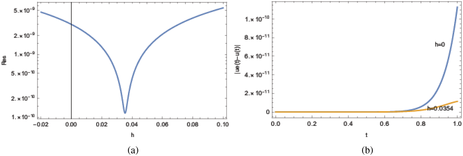
Figure 2: ADM solutions for Example 2 at the approximation level 6. (a) Residual error and (b) pointwise errors

For future reference, the approximate analytical solution from the 6th order modified ADM method used to generate the above results is given by Eq. (19):

u(t)=t2+1.38778×10−17t39/10+4.33681×10−19t49/10+2.60209×10−18t29/5−1.35525×10−19t34/5−5.42101×10−20t77/10−1.69407×10−21t87/10+8.47033×10−22t48/5−9.92617×10−24t53/5−6.61744×10−24t23/2+1.24125×10−10t25/2−1.12727×10−10t67/5. (19)

Example 3. The nonlinear logistic growth fractional differential equation studied in [19,40] is next accounted in the form

u(α)(t)=14u(t)(1−u(t)),u(0)=1/3,0≤t≤17. (20)

For comparison purposes with the literature, the exact solution to Eq. (20) with α=1, which is ue(t)=et/42+et/4, is analyzed in detail in what follows. The resulting ADM iterationsEq. (11) for the problem Eq. (20) are now in the format

u0=13−ht,u1=I(α)(14u0(t)(1−u0(t)))+ht,un+1=I(α)(14(un(t)−An(t))),n≥1. (21)

With 6 number of terms in the ADM series, the ADM method Eq. (21) produces the optimum h value −0.0509 and the resulting squared residual error with the larger interval of integration domain in Eq. (20) is Res = 0.00719. The same is Res = 0.4594 in the case of classical ADM with h = 0, refer to Fig. 3a. The absolute pointwise error in Fig. 3b and the full approximate solutions against the exact one in Fig. 3c also justify the power the new ADM. Notice in Fig. 3c that the classical ADM will fail to be convergent to the physical solution in the domain of definition. Hence, a great improvement with embedding functional into the traditional ADM is achieved here.

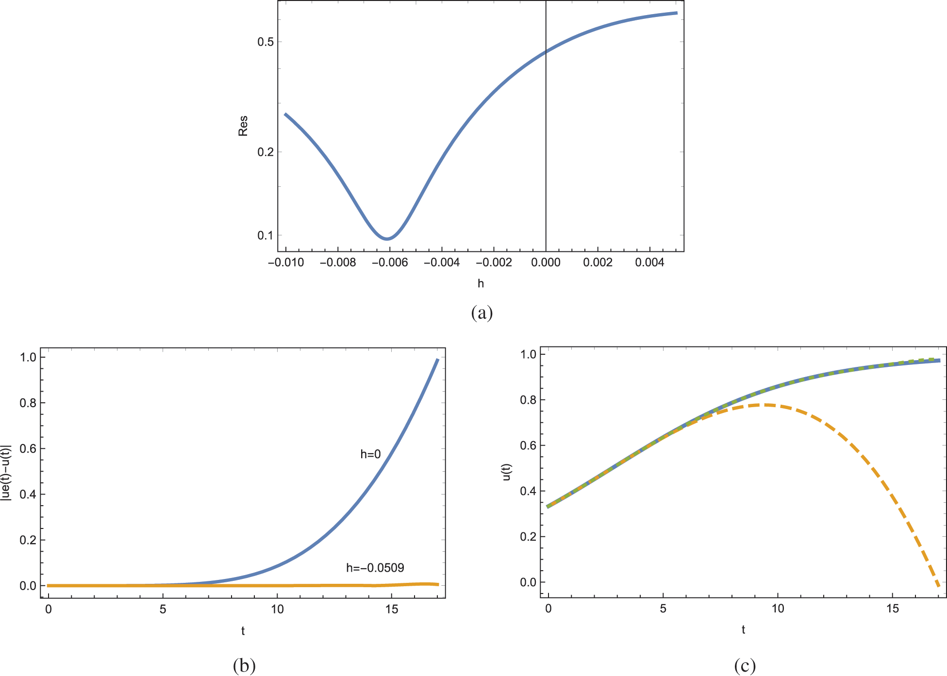
Figure 3: ADM solutions for Example 3 at the approximation level 6. (a) Residual error, (b) pointwise errors and (c) solutions; unbroken is exact, dashed is the traditional ADM and dotted is the present ADM

Actually, doubling the number of terms gives an improved optimal h value −0.0508, which yields a smaller residual error Res = 0.00023, hence reducing the error by an order of magnitude ten. The corresponding data is eventually exhibited through Figs. 4a–4c for further visualization. It is remarked that, even taking twice as large number of terms in the ADM series will not save the classical ADM diverting from the full physical solution, as inferred from Fig. 4c. Indeed, the corresponding residual error increases to Res = 29.49. However, a smooth convergence of the improved ADM solution is guaranteed as seen from the non distinguishable dotted curve in Fig. 4c.

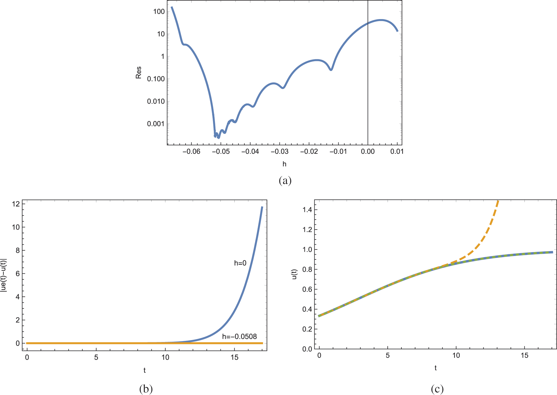
Figure 4: ADM solutions for Example 3 at the approximation level 12. (a) Residual error, (b) pointwise errors and (c) solutions; unbroken is exact, dashed is the traditional ADM and dotted is the present ADM

Example 4. We consider now the ordinary fractional half-order nonlinear differential equation given in [15]

u′+u(1/2)−u2=1+2πt1/2−t2,u(0)=0,0≤t≤2, (22)

with the exact solution ue(t) = t. The proposed accelerated ADM inEq. (11) for the present problem in Eq. (22) turns out to be

u0=(1−h)∫0t(1+2πt1/2−t2)dt,u1=h∫0t(1+2πt1/2−t2)dt−(I1/2u0)(t)+∫0tA0(t)dt,un+1=−(I(1/2)un)(t)+∫0tAn(t)dt,n≥1, (23)

for which the Adomian polynomials An′s are for the nonlinearity u2.

The residual error is displayed in Fig. 5a and the pointwise errors are revealed in Fig. 5b. At the approximation level M = 3, the classical ADM in [15] with h = 0 in Eq. (23) gives a residual error from Eq. (12) as Res = 0.98, whereas it is lowered to Res = 0.047 with the optimal h as 0.218 obtained from the present approach. So, an advantage of 10−2 in the error is reached by the parameter embedding into the classical ADM, as observed from Fig. 5b. For instance, the error |u(2) − ue(2)| = 0.230932 obtained from the traditional ADM in [15] with h = 0 is reduced to |u(2) − ue(2)| = 0.001019 within the present ADM. This advantage will certainly be much improved as the order of Adomian polynomials is increased.

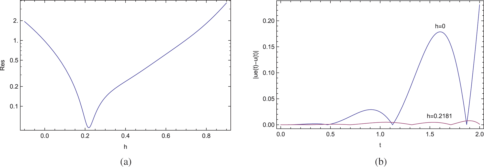
Figure 5: ADM solutions for Example 4 at the approximation level 3. (a) Residual error and (b) pointwise errors

Example 5. In this example, it is accounted for the ordinary fractional order nonlinear differential equation version of the classical free-fall mechanical problem (when m = 1) often studied in the open literature such as [12]

u(α)+u2=1,0≤t≤1,u(0)=⋯=u(kα)(0)=0,(k=0,1⋯,m−1),m−1<α≤m,m∈N. (24)

The proposed accelerated ADM inEq. (11) for the present problem in Eq. (24) becomes

u0=Iα(1)−htα,u1=htα−(IαA0)(t),un+1=−(IαAn)(t),n≥1, (25)

for which the Adomian polynomials An′s are for the nonlinearity u2. Some of the iterations from Eq. (25) are presented below in Eq. (26)

u0=tα(−h+1Γ(1+α)),u1=htα−t3α(−1+hΓ(1+α))2Γ(1+2α)Γ(1+α)2Γ(1+3α),u2=2t3α(−1+hΓ(1+α))Γ(1+2α)(−t2α(−1+hΓ(1+α))2Γ(1+4α)+hΓ(1+α)2Γ(1+5α))Γ(1+α)3Γ(1+3α)Γ(1+5α),u3=t3αΓ(1+2α)Γ(1+3α)2(−h2Γ(1+3α)+6ht2α(−1+hΓ(1+α))2Γ(1+3α)Γ(1+4α)Γ(1+α)2Γ(1+5α)−t4α(−1+hΓ(1+α))4(4Γ(1+3α)Γ(1+4α)+Γ(1+2α)Γ(1+5α))Γ(1+6α)Γ(1+α)4Γ(1+5α)Γ(1+7α)). (26)

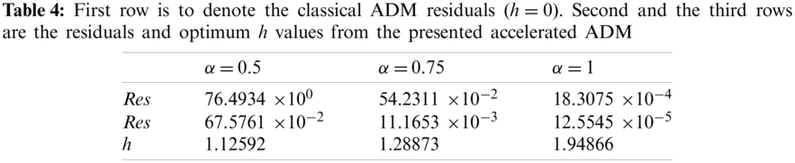
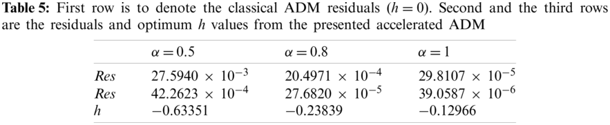
Minimizing the residuals as shown in Fig. 6a for three distinct values of the exponent α at the approximation level M = 8, the corresponding optimal values of h are listed in Table 3. The present technique clearly enhances the accuracy over the classical ADM method.

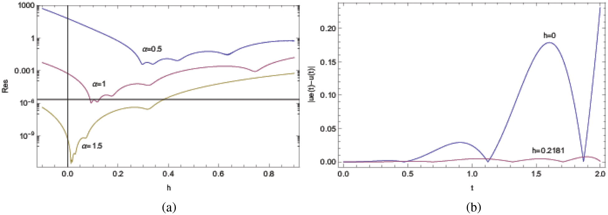
Figure 6: ADM solutions for Example 5 at the approximation level 8. (a) Residual error and (b) Approximate solutions

The approximate solutions are further demonstrated in Fig. 6b, for which α=1 leads to the exact solution u=tanh⁡t.

3.2 Partial Fractional Differential Equations

Example 1. Consider the single nonlinear fractional reaction-diffusion equation as presented in [10]

Dt(α)u=(u2ux)x−u−u3,0≤t≤2,0≤x≤5,0<α≤1u(x,0)=ex3. (27)

The system in Eq. (27) has exact traveling-wave solution when α=1 expressed by u(x,t)=e−t+x3. In this case we have the iterative procedure due to the improved ADM inEq. (11)

u0=(1−ht)ex3,u1=htex3+∫0tA0(x,t)dt,un+1=∫0tAn(x,t)dt,n≥1, (28)

for which the Adomian polynomials An′s are representing the right-hand side of Eq. (27). The tenth-order ADM approximation from Eq. (28) yields the approximate solution Eq. (29)

u(x,t)=ex3(1−t+t22−t36+t424−t5120+t6720−t75040+t840320−t9362880+t103628800−ht1139916800). (29)

At this level of ADM series, minimizing the squared residual error over the domain x∈[0,5] and t∈[0,2] using Eq. (12), we obtain an optimum value of h = 0.85207 leading to the residual error 9.76516×10−6 vs. the classical ADM residual 1.45122×10−3 with h = 0. This can be better visualized from Fig. 7. Indeed, the values of u(5, 2) from the classical ADM, from the present ADM and from the exact formula result in 2.428019036, 2.427234972, 2.427231593, respectively.

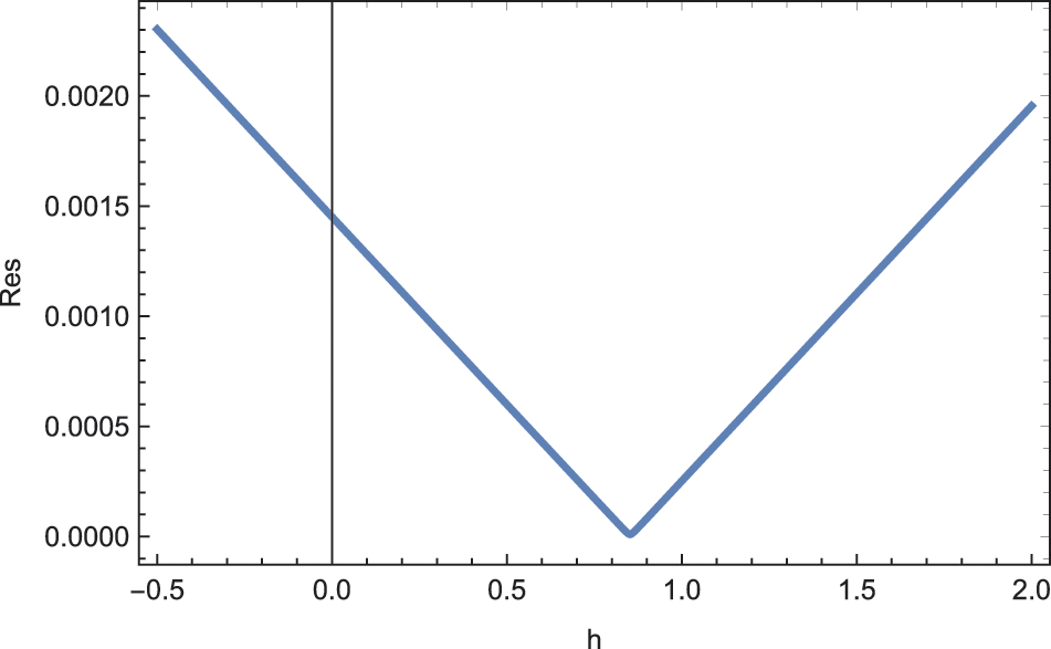
Figure 7: ADM solutions for Example 1 at the approximation level 10 displaying the residual error

Example 2. We now deal with the time-fractional Fornberg-Whitham partial differential equation as presented in [13]

Dt(α)u+Lu+Nu=0,0≤t≤6,0≤x≤4,0<α≤1u(x,0)=e12x, (30)

where Lu = − uxxt + ux is the linear and Nu=12(u2−uxx2)x is the nonlinear components. We have the present ADM iterative process for Eq. (30) generating Eq. (31)

u0=(1−ht)e12x,u1=hte12x−Iα(Lu0(x,t)+A0(x,t)),un+1=−Iα(Lun(x,t)+An(x,t)),n≥1, (31)

where An′s are the Adomian polynomials representing the nonlinearity N in Eq. (30).

The fifth-order ADM series approximation generates an optimum value of h = 0.41681 for the derivative-order α=1 and of h = 0.34137 for the fractional derivative-order α=0.9, whose residuals can be observed in Fig. 8. With the advantage of reduction of the error by the order of magnitude 10−1, the present ADM will receive the error of the Homotopy Analysis method given in [13].

Example 3. We now consider the following time-fractional Navier-Stokes equation for the diffusion model given in [9]

Dt(α)u=urr+1rur,0≤t≤1,4≤r≤∞,0<α≤1u(r,0)=r. (32)

The iterative ADM adopted for Eq. (32) is

u0=(1−h)r,u1=hr+(IαLu0)(r,t),un+1=(IαLun)(r,t),n≥1, (33)

with Lu=urr+1rur. Eq. (33) produces at the tenth-order of approximation Eq. (34)

u(r,t)=1r19(r20+r18tαΓ(1+α]+r16t2αΓ(1+2α)+9t3α(r14Γ(1+3α)+25tα(r12Γ(1+4α)+49tα(r10Γ(1+5α)+81tα(r8Γ(1+6α)+121tα(r6Γ(1+7α)+169tα(r4Γ(1+8α)+225tα(r2Γ(1+9α)−289(−1+h)tαΓ(1+10α))))))))). (34)

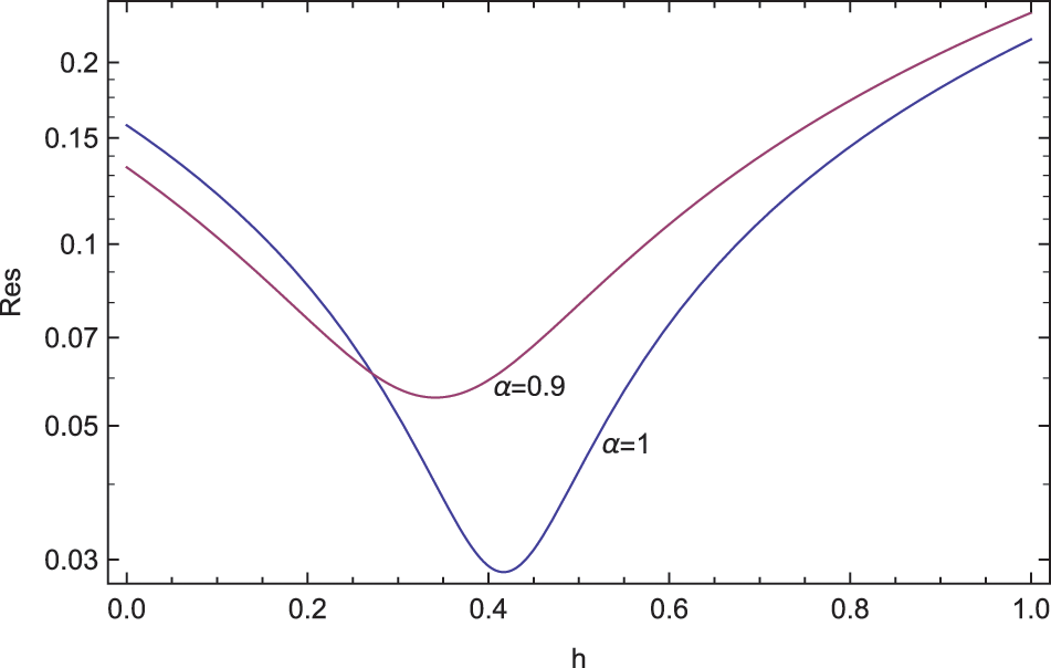
Figure 8: ADM solutions for Example 2 at the approximation level 5 displaying the residual error

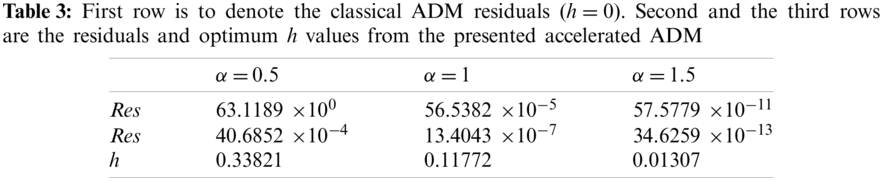
Fig. 9 reveals the residuals, respectively for α=0.5, 0.75 and 1. The optimal values of h are also summarized in Table 4. The advantage of the present ADM is anticipated.

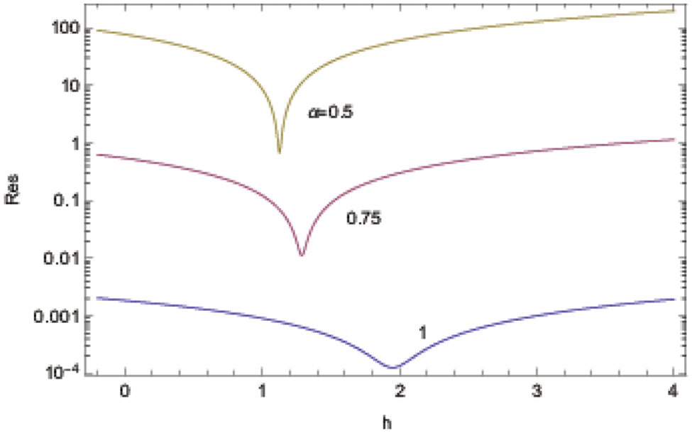
Figure 9: ADM solutions for Example 3 at the approximation level 10 displaying the residual error

Example 4. We finally consider the following cancer tumor model given in [5]

Dt(α)u=urr−t2u,0≤t≤1,0≤r≤∞,0<α≤1u(r,0)=e−r. (35)

Model in Eq. (35) is treated with the present ADM procedure in Eq. (36)

u0=(1−h)e−r,u1=he−r+(IαLu0)(r,t),un+1=(IαLun)(r,t),n≥1, (36)

with Lu = urr − t2u.

Fig. 10 reveals the residuals, respectively for α=0.5, 0.8 and 1. The corresponding optimal values of h are further summarized in Table 5. We observe the contribution of the proposed technique to the accuracy via the addition of h.

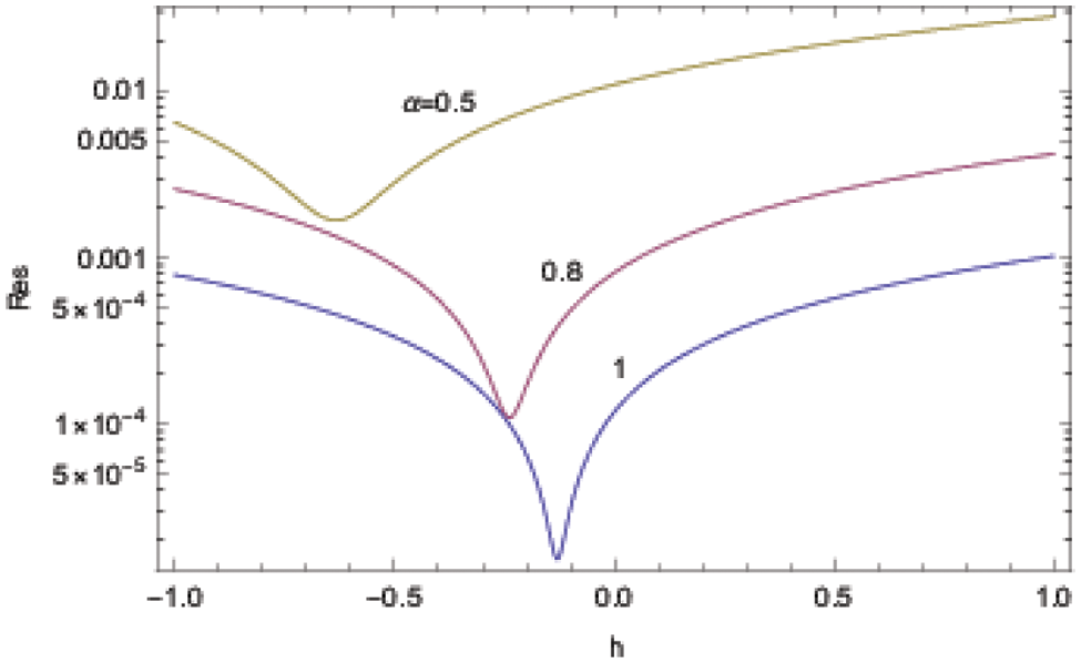
Figure 10: ADM solutions for Example 4 at the approximation level 5 displaying the residual error

Remark 2. For numerical examples ofr fractional partial differential equations, only initial problems are given due to the fact that the fractional derivatives are assigned to the time derivative. However, the modified ADM procedure is also equally applicable when fractional partial differential equations are considered with initial and boundary conditions.

4  Conclusions

The motivation of the present work is to provide an effective solution method for the fractional ordinary and partial differential equations of the hot topic of the recent literature. A considerable performance the present approach over the standard ADM is obtained by means of plugging a functional term involving both a variable and a parameter. L2 norm is then adopted in order for capturing the optimal embedded parameter value by means of the global error from the squared residual. The advantage of the proposed method is tested over well-studied ordinary and partial fractional differential equations involving a variety of fractional order derivatives. Results prove that the presented algorithm is fairly accurate, more advantageous over the traditional ADM as well as over some recent numerical approaches and also more straightforward to implement for the fractional differential equations. Indeed, the functional term embedding adopted here is shown to greatly accelerate the convergence of the conventional ADM series in the problems involving both fractional ordinary and partial differential equations analyzed here.

As a future research, the current proposal can be extended to variable order fractional differential equations. This will obviously require more mathematical rigor. Other functional embeddings from the considered here can be searched for improving the accuracy of the Adomian decomposition method as well. Moreover, the linear/nonlinear PDEs considered within the present research involve (1+1) (time+space) dimensional equations. Application of the present ADM modification to (1+2) and higher-dimensional equations would warrant further work.

Funding Statement: The author received no specific funding for this study.

Conflicts of Interest: The author declares that he has no conflicts of interest to report regarding the present study.

References

 1.  Podlubny, I. (1999). Fractional differential equations: An introduction to fractional derivatives. New York: Academic Press. [Google Scholar]

 2.  Atkinson, C., Osseiran, A. (2011). Rational solutions for the time-fractional diffusion equation. SIAM Journal of Applied Mathematics, 71(1), 92–106. DOI 10.1137/100799307. [Google Scholar] [CrossRef]

 3.  Bolat, Y. (2014). On the oscillation of fractional-order delay differential equations with constant coefficients. Communications in Nonlinear Science and Numerical Simulation, 19(11), 3988–3993. DOI 10.1016/j.cnsns.2014.01.005. [Google Scholar] [CrossRef]

 4.  Su, N. (2014). Mass-time and space-time fractional partial differential equations of water movement in soils: Theoretical framework and application to infiltration. Journal of Hydrology, 519, 1792–1803. DOI 10.1016/j.jhydrol.2014.09.021. [Google Scholar] [CrossRef]

 5.  Iyiola, O. S., Zaman, F. D. (2014). A fractional diffusion equation model for cancer tumor. AIP Advances, 4(10), 107121. DOI 10.1063/1.4898331. [Google Scholar] [CrossRef]

 6.  Carvalho-Neto, P. M., Planas, G. (2015). Mild solutions to the time fractional Navier-Stokes equations in RN. Journal of Differential Equations, 259(7), 2948–2980. DOI 10.1016/j.jde.2015.04.008. [Google Scholar] [CrossRef]

 7.  Zhang, X., Zhang, B., Repovs, D. (2016). Existence and symmetry of solutions for critical fractional schrödinger equations with bounded potentials. Nonlinear Analysis: Theory, Methods & Applications, 142, 48–68. DOI 10.1016/j.na.2016.04.012. [Google Scholar] [CrossRef]

 8.  Abro, K. A., Khan, I., Tassaddiq, A. (2018). Application of Atangana-Baleanu fractional derivative to convection flow of MHD Maxwell fluid in a porous medium over a vertical plate. Mathematical Modelling of Natural Phenomena, 13, 1. DOI 10.1051/mmnp/2018007. [Google Scholar] [CrossRef]

 9.  Momani, S., Odibat, Z. (2006). Analytical solution of a time-fractional Navier-Stokes equation by Adomian decomposition method. Applied Mathematics and Computation, 177(2), 488–494. DOI 10.1016/j.amc.2005.11.025. [Google Scholar] [CrossRef]

10. Song, L., Wang, W. (2013). A new improved Adomian decomposition method and its application to fractional differential equations. Applied Mathematical Modelling, 37(3), 1590–1598. DOI 10.1016/j.apm.2012.03.016. [Google Scholar] [CrossRef]

11. Turkyilmazoglu, M. (2021). Nonlinear problems via a convergence accelerated Decomposition Method of Adomian. Computer Modeling in Engineering & Sciences, 127(1), 1–22. DOI 10.32604/cmes.2021.012595. [Google Scholar] [CrossRef]

12. Ji, J., Zhang, J., Donga, Y. (2012). The fractional variational iteration method improved with the Adomian series. Applied Mathematics Letters, 25(12), 2223–2226. DOI 10.1016/j.aml.2012.06.007. [Google Scholar] [CrossRef]

13. Sakar, M. G., Erdogan, F. (2013). The homotopy analysis method for solving the time-fractional Fornberg-Whitham equation and comparison with adomian’s decomposition method. Applied Mathematical Modelling, 37(20–21), 8876–8885. DOI 10.1016/j.apm.2013.03.074. [Google Scholar] [CrossRef]

14. Turkyilmazoglu, M. (2019). Equivalence of ratio and residual approaches in the homotopy analysis method and some applications in nonlinear science and engineering. Computer Modeling in Engineering & Sciences, 120(1), 63–81. DOI 10.32604/cmes.2019.06858. [Google Scholar] [CrossRef]

15. Mohamed, A. S., Mahmoud, R. A. (2016). Picard, Adomian and predictor-corrector methods for an initial value problem of arbitrary (fractional) orders differential equation. Journal of the Egyptian Mathematical Society, 28(2), 165–170. DOI 10.1016/J.JOEMS.2015.01.001. [Google Scholar] [CrossRef]

16. Li, M., Gu, X. M., Huang, C., Fei, M., Zhang, G., (2018). A fast linearized conservative finite element method for the strongly coupled nonlinear fractional equations. Journal of Computational Physics, 358, 256–282. DOI 10.1016/j.jcp.2017.12.044. [Google Scholar] [CrossRef]

17. Ford, N. J., Connolly, J. A. (2006). Comparison of numerical methods for fractional differential equation. Communications on Pure and Applied Analysis, 5(2), 289–307. DOI 10.3934/cpaa.2006.5.289. [Google Scholar] [CrossRef]

18. Esmaeili, S., Shamsi, M., Luchko, Y. (2011). Numerical solution of fractional differential equations with a collocation method based on Mn¨z polynomials. Computers and Mathematics with Applications, 62(3), 918–929. DOI 10.1016/j.camwa.2011.04.023. [Google Scholar] [CrossRef]

19. Bhalekar, A., Daftardar-Geji, V. (2012). Solving fractional-order logistic equation using a new iterative method. International Journal of Differential Equations, 2012, 975829. DOI 10.1155/2012/975829. [Google Scholar] [CrossRef]

20. Akgul, A., Inc, M., Karatas, E., Baleanu, D. (2015). Numerical solutions of fractional differential equations of Lane-Emden type by an accurate technique. Advances in Difference Equations, 2015(1), 220. DOI 10.1186/s13662-015-0558-8. [Google Scholar] [CrossRef]

21. Albadarneh, R. B., Batiha, I. M., Zurigat, M. (2016). Numerical solutions for linear fractional differential equations of order 1<α<2 using finite difference method (FFDM). Journal of Mathematics and Computer Science, 16(1), 103–111. [Google Scholar]

22. Daraghmeh, A., Qatanani, M., Saadeh, A. (2020). Numerical solution of fractional differential equations. Applied Mathematics, 11(11), 1100–1115. DOI 10.4236/am.2020.1111074. [Google Scholar] [CrossRef]

23. Alchikh, R., Khuri, S. A. (2020). Numerical solution of a fractional differential equation arising in optics. Optik–International Journal for Light and Electron Optics, 208, 163911. DOI 10.1016/j.ijleo.2019.163911. [Google Scholar] [CrossRef]

24. Kumar, S. (2021). Fractional fuzzy model of advection-reaction-diffusion equation with application in porous media. Journal of Porous Media (in Press). DOI 10.1615/JPorMedia.2021034897. [Google Scholar] [CrossRef]

25. Kumar, S. (2020). Numerical solution of fuzzy fractional diffusion equation by Chebyshev spectral method. Numerical Methods for Partial Differential Equations, 1–19. DOI 10.1002/num.22650. [Google Scholar] [CrossRef]

26. Kumar, S., Nieto, J. J., Ahmad, B. (2022). Chebyshev spectral method for solving fuzzy fractional Fredholm-Volterra integro-differential equation. Mathematics and Computers in Simulation, 192(6), 501–513. DOI 10.1016/j.matcom.2021.09.017. [Google Scholar] [CrossRef]

27. Kumar, S., Zeidan, D. (2021). An efficient Mittag-Leffler kernel approach for time-fractional advection-reaction-diffusion equation. Applied Numerical Mathematics, 170, 190–207. DOI 10.1016/j.apnum.2021.07.025. [Google Scholar] [CrossRef]

28. Kumar, S., Zeidan, D. (2022). Numerical study of Zika model as a mosquito-borne virus with non-singular fractional derivative. International Journal of Biomathematics (in Press). DOI 10.1142/S1793524522500188. [Google Scholar] [CrossRef]

29. Kammanee, A. (2021). Numerical solutions of fractional differential equations with variable coeffcients by taylor basis functions. Kyungpook Mathematical Journal, 61, 383–393. DOI 10.5666/KMJ.2021.61.2.383. [Google Scholar] [CrossRef]

30. Ahsan, S., Nawaz, R., Akbar, M., Nisar, K. S., Abualnaja, K. M. et al. (2021). Numerical solution of two-dimensional fractional order volterra integro-differential equations. AIP Advances, 11(3), 035232. DOI 10.1063/5.0032636. [Google Scholar] [CrossRef]

31. Hammad, H. A., Aydi, H., Sen, M. D. l. (2021). Solutions of fractional differential type equations by fixed point techniques for multivalued contractions. Complexity, 2021, 5730853. DOI 10.1155/2021/5730853. [Google Scholar] [CrossRef]

32. Asl, M. S., Javidi, M., Yan, Y. (2021). High order algorithms for numerical solution of fractional differential equations. Advances in Difference Equations, 2021, 111. DOI 10.1186/s13662-021-03273-4. [Google Scholar] [CrossRef]

33. Gande, N. R., Madduri, H. (2022). Higher order numerical schemes for the solution of fractional delay differential equations. Journal of Computational and Applied Mathematics, 402, 113810. DOI 10.1016/j.cam.2021.113810. [Google Scholar] [CrossRef]

34. Chouhan, D., Mishra, V., Srivastava, H. M. (2021). Bernoulli wavelet method for numerical solution of anomalous infiltration and diffusion modeling by nonlinear fractional differential equations of variable order. Results in Applied Mathematics, 10, 100146. DOI 10.1016/j.rinam.2021.100146. [Google Scholar] [CrossRef]

35. Postavaru, O., Toma, A. (2021). Numerical solution of two-dimensional fractional-order partial differential equations using hybrid functions. Partial Differential Equations in Applied Mathematics, 4, 100099. DOI 10.1016/j.padiff.2021.100099. [Google Scholar] [CrossRef]

36. Amin, R., Shah, K., Asif, M., Khan, I. (2021). A computational algorithm for the numerical solution of fractional order delay differential equations. Applied Mathematics and Computation, 402, 125863. DOI 10.1016/j.amc.2020.125863. [Google Scholar] [CrossRef]

37. Duan, J. S., Chaolu, T., Rach, R., Lu, L. (2013). The Adomian decomposition method with convergence acceleration techniques for nonlinear fractional differential equations. Computers and Mathematics with Applications, 66(5), 728–736. DOI 10.1016/j.camwa.2013.01.019. [Google Scholar] [CrossRef]

38. Adomian, G. (1994). Solving frontier problems of physics: The decomposition method. Dordrecht: Kluwer Academic Publishers. [Google Scholar]

39. Cherruault, Y., Adomian, G. (1993). Decomposition methods: A new proof of convergence. Mathematical and Computer Modelling, 18(12), 103–106. DOI 10.1016/0895-7177(93)90233-O. [Google Scholar] [CrossRef]

40. Gunerhan, H., Yigider, M., Manafian, J., Ilhan, O. A. (2021). Numerical solution of fractional order logistic equations via conformable fractional differential transform method. Journal of Interdisciplinary Mathematics, 24(5), 1207–1220. DOI 10.1080/09720502.2021.1918319. [Google Scholar] [CrossRef]

This work is licensed under a Creative Commons Attribution 4.0 International License, which permits unrestricted use, distribution, and reproduction in any medium, provided the original work is properly cited.