| Computer Modeling in Engineering & Sciences |
DOI: 10.32604/cmes.2022.021299
ARTICLE
Cotangent Similarity Measure of Consistent Neutrosophic Sets and Application to Multiple Attribute Decision-Making Problems in Neutrosophic Multi-Valued Setting
1School of Mechatronic Engineering and Automation, Shanghai University, Shanghai, 200444, China
2Department of Computer Science and Engineering, Shaoxing University, Shaoxing, 312000, China
3Zhejiang Industry Polytechnic College, Shaoxing, 312000, China
*Corresponding Author: Bing Wang. Email: susanbwang@shu.edu.cn
Received: 06 January 2022; Accepted: 10 March 2022
Abstract: A neutrosophic multi-valued set (NMVS) is a crucial representation for true, false, and indeterminate multi-valued information. Then, a consistent single-valued neutrosophic set (CSVNS) can effectively reflect the mean and consistency degree of true, false, and indeterminate multi-valued sequences and solve the operational issues between different multi-valued sequence lengths in NMVS. However, there has been no research on consistent single-valued neutrosophic similarity measures in the existing literature. This paper proposes cotangent similarity measures and weighted cotangent similarity measures between CSVNSs based on cotangent function in the neutrosophic multi-valued setting. The cosine similarity measures show the cosine of the angle between two vectors projected into a multidimensional space, rather than their distance. The cotangent similarity measures in this study can alleviate several shortcomings of cosine similarity measures in vector space to a certain extent. Then, a decision-making approach is presented in view of the established cotangent similarity measures in the case of NMVSs. Finally, the developed decision-making approach is applied to selection problems of potential cars. The proposed approach has obtained two different results, which have the same sort sequence as the compared literature. The decision results prove its validity and effectiveness. Meantime, it also provides a new manner for neutrosophic multi-valued decision-making issues.
Keywords: Neutrosophic multi-valued set; consistency single-valued neutrosophic sets; cotangent similarity measure; multiple attribute decision-making
Zadeh [1] proposed fuzzy sets for the first time to deal with fuzzy information in uncertain problems. Atanassow [2] further extended the fuzzy set and proposed the intuitionistic fuzzy set, which is described by a membership degree and a nonmembership degree. Smarandache [3] proposed the concept of a neutrosophic set (NS) considering the truth, falsity, and determinacy membership degrees. NS shows its main merit in dealing with indeterminate and inconsistent information. Hence, NSs have been widely used in image segmentation [4,5], decision making [6], clustering analysis [7], and so on. Wang et al. [8] introduced the concept of a single-valued neutrosophic set (SVNS) within the real interval [0,1] to more effectively solve practical problems. For example, some similarity measures of SVNSs were applied in multiple attribute decision-making (MADM) [9,10] and clustering analysis [11]. Then, the cross entropy of SVNSs was utilized for MADM [12] and object tracking [13]. Some aggregation operators of SVNSs and correlation coefficients of SVNSs were used for MADM [14,15]. As the subclass of NS, some aggregation operators of simplified NSs (containing SVNSs and interval NSs) [16–18] and similarity measures of simplified NSs [19] were presented and used for MADM.
When considering neutrosophic multi-valued/hesitant information, some similarity measures of single-valued neutrosophic multisets (SVNMs) were proposed and used for medical diagnosis [20] and MADM [21]. Multi-valued/hesitant NSs were introduced and applied in decision-making [22–29]. However, MVNS loses some identical neutrosophic values due to hesitant characteristics, thus the information aggregation of MVNSs may produce the union of multiple aggregated values in MADM problems, which may lead to computational complexity [24]. Furthermore, converting single-valued neutrosophic sequences in SVNM into SVNS [21] only contains the average value in the transformation process, which may lead to the loss of useful information (e.g., standard deviation). To solve these issues, Ye et al. [30] proposed a neutrosophic multi-valued set (NMVS), which contains identical and/or different true, false and indeterminate values, and defined a new method that converts NMVS into consistent single-valued neutrosophic sets (CSVNSs) in view of the mean and consistent degree of the true, false and indeterminate sequences. They also introduced the correlation coefficients of CSVNSs and applied them to MADM.
However, a similarity measure for CSVNSs was studied in the literature [30] as it is a key mathematical tool for MADM problems in the setting of NMVSs. Therefore, we should propose new similarity measures of CSVNSs to perform MADM in the case of NMVSs. In this paper, two cotangent similarity measures of NMVSs are proposed and applied to the purchase decision issue of potential cars. The rest of the paper consists of the following sections. Section 2 introduces some concepts of NMVSs and CSVNSs. The cotangent similarity measures of the CSVNSs are established from the cotangent function, and the properties of the cotangent similarity measures are demonstrated in Section 3. Section 4 introduces the MADM algorithm with respect to the established cotangent similarity measures of CSVNSs. Section 5 presents an example of purchase decision issues of potential cars and the comparative results of the related approach to prove the effectiveness and rationality of the new approach. Finally, conclusions and further works are put forward in Section 6.
2 Some Concepts of NMVSs and CSVNSs
This section introduces some concepts of NMVSs and CSVNSs presented by Ye et al. [30].
Definition 2.1 [30]. Let D = {d1, d2, …, ds} be a finite set. A NMVS Y defined on D is given by
where NFY (dj), NIY (dj) and NTY (dj) are the falsity-membership function, the indeterminacy membership function, and the truth membership function, respectively, which are described by three multi-valued sequences
The basic element <dj, NTY(dj), NIY(dj), NFY(dj)> (j = 1, 2, …, s) in Y is simply denoted as
Definition 2.2 [30]. Set Y = {y1, y2, …, ys} as NMVS, where
where δNTj, δNIj, δNFj
For two CSVNEs gj = <(nNTj, bNTj), (nNIj, bNIj), (nNFj, bNFj)> (j = 1, 2), both contain the following relationships:
(1) If g1 ⊆ g2, there are nNT1 ≤ nNT2, nNI1 ≥ nNI2, nNF1 ≥ nNF2, bNT1 ≤ bNT2, bNI1 ≥ bNI2, and bNF1 ≥ bNF2;
(2) If g1 ⊆ g2 and g2 ⊆ g1, there are nNT1 = nNT2, nNI1 = nNI2, nNF1 = nNF2, bNT1 = bNT2, bNI1 = bNI2, and bNF1 = bNF2.
By means of the average values of NTj, NIj and NFj and the consistent degrees of NTj, NIj, and NFj, weighted correlation coefficients between CSVNSs are introduced below [30].
Definition 2.3 [30]. Set Y1 = {y11, y12, …, y1s} and Y2 = {y21, y22, …, y2s} as two NMVSs, where
where bNTij, bNIij, bNFij, nNTij, nNIij, and nNFij are the consistent degrees and average values of NTij, NIij, and NFij (i = 1, 2; j = 1, 2, …, s), which are produced by Eqs. (2)–(7).
3 Cotangent Similarity Measures of CSVNSs
This section introduces cotangent similarity measures and weighted cotangent similarity measures between CSVNSs and their properties.
Definition 3.1. Let Y1 = {y11, y12, …, y1s} and Y2 = {y21, y22, …, y2s} be two NMVSs, where
where bNTj, bNIj, bNFj, nNTj, nNIj, and nNFj are the consistent degrees and average values of NTij, NIij, and NFij, which are produced by Eqs. (2)–(7).
Proposition 3.1. The cotangent similarity measures Cot1(G1, G2) and Cot2(G1, G2) in CSVNSs have the following properties:
(Z1) Cot1(G1, G2) = Cot1(G2, G1) and Cot2(G1, G2) = Cot2(G2, G1);
(Z2) 0 ≤ Cot1(G1, G2), Cot2(G1, G2) ≤ 1;
(Z3) Cot1(G1, G2) = 1 if only if G1 = G2;
(Z4) For any CSVNS G3 and G1 ⊆ G2 ⊆ G3, Cot1(G1, G2) ≥ Cot1(G1, G3) and Cot2(G2, G3) ≥ Cot2(G1, G3).
Proof: (Z1) It is obvious that the proof of the property (Z1) is straightforward.
(Z2) Since the values of |nNT1j − nNT2j|, |nNI1j − nNI2j|, |nNF1j − nNF2j|, |bNT1j − bNT2j|, |bNI1j − bNI2j| and |bNF1j − bNF2j| for j = 1, 2, …, s are between 0 and 1 and the value of cotangent function falls in the interval [π/4, π/2], the cotangent values in Eqs. (10) and (11) are also located between 0 and 1. Hence, there is 0 ≤ Coti(G1, G2) ≤ 1 for i = 1, 2.
(Z3) For the two CSVNSs G1 and G2, if G1 = G2, this implies nNT1j = nNT2j, nNI1j = nNI2j, nNF1j = nNF2j, bNT1j = bNT2j, bNI1j = bNI2j and bNF1j = bNF2j for j = 1, 2, …, s. Hence |nNT1j − nNT2j| = 0, |nNI1j − nNI2j| = 0, |nNF1j − nNF2j| = 0, |bNT1j − bNT2j| = 0, |bNI1j − bNI2j| = 0, and |bNF1j − bNF2j| = 0. Thus Coti(G1, G2) = 1 for i = 1, 2.
If Coti(G1, G2) = 1 for i = 1, 2, this implies cot(π/4) = 1 and |nNT1j - nNT2j| = 0, |nNI1j - nNI2j| = 0, |nNF1j − nNF2j| = 0, |bNT1j − bNT2j| = 0, |bNI1j − bNI2j| = 0, and |bNF1j − bNF2j| = 0 for j = 1, 2, …, s. Then, there are nNT1j = nNT2j, nNI1j = nNI2j, nNF1j = nNF2j, bNT1j = bNT2j, bNI1j = bNI2j and bNF1j = bNF2j for j = 1, 2, …, s. Therefore, there is G1 = G2.
(Z4) Since there exists G1 ⊆ G2 ⊆ G3, there are |nNT1j − nNT3j| ≥ |nNT1j − nNT2j|, |nNT1j − nNT3j| ≥ |nNT2j − nNT3j|, |nNI1j − nNI3j| ≥ |nNI1j − nNI2j|, |nNI1j − nNI3j| ≥ |nNI2j − nNI3j|, |nNF1j − nNF3j| ≥ |nNF1j − nNF2j|, |nNF1j − nNF3j| ≥ |nNF2j − nNF3j|, |bNT1j − bNT3j| ≥ |bNT1j − bNT2j|, |bNT1j − bNT3j| ≥ |bNT2j − bNT3j|, |bNI1j − bNI3j| ≥ |bNI1j −bNI2j|, |bNI1j − bNI3j| ≥ |bNI2j − bNI3j|, |bNF1j − bNF3j| ≥ |bNF1j − bNF2j|, and |bNF1j − bNF3j| ≥ |bNF2j − bNF3j|. Since the cotangent function is a decreasing function within the interval [π/4, π/2], there are Cot1(G1, G2) ≥ Cot1(G1, G3) and Cot2(G2, G3) ≥ Cot2(G1, G3).
When the importance of each yij is different, the weight of yij (i = 1, 2; j = 1, 2, …, s) is specified as wj with wj ∈ [0,1] and
When wj =1/s (j = 1, 2, …, s), Eqs. (12) and (13) are reduced to Eqs. (10) and (11), which are special cases of Eqs. (12) and (13).
4 MADM Approach Regarding the Proposed Cotangent Similarity Measures of CSVNSs
This part introduces a MADM approach corresponding to the proposed cotangent similarity measures in the setting of NMVSs. When dealing with a MADM problem, there is often a set of multiple alternatives T = {T1, T2, …, Tq}, evaluated by a group of multiple attributes E = {e1, e2, …, es}. The weight vector of E is specified as w = (w1, w2, …, ws). Each alternative Ti (i = 1, 2, …, q) is evaluated over the attributes ej by a NMVE
Step 1: Using Eqs. (2)–(7), the NMVS Yi = {yi1, yi2, …, yis} and the decision matrix Y = (yij)q.s are transformed into the CSVNS Gi = {gi1, gi2, …, gis} and the decision matrix of CSVNSs G = (gij)q.s, respectively.
Step 2: The ideal solution
Step 3: The weighted cotangent similarity measures of the CSVNSs Gi and G * for Ti are obtained by the following equations:
or
Step 4: According to the values of the weighted cotangent similarity measure, the alternatives are arranged in descending order, and the best one is selected.
Step 5: End.
To easily compare the proposed MADM approach with existing relevant MADM methods, this section presents an illustrative example on the selection purchase of potential cars in [21] to illustrate the effectiveness and rationality of the proposed MADM approach.
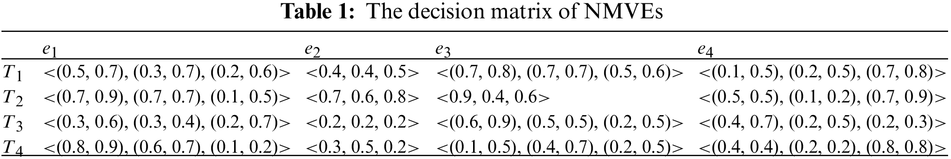
Customers want to choose a suitable car according to their own living needs and driving habits. There are four types of potential cars, represented by the set of alternatives T = {T1, T2, T3, T4}. They must satisfy the requirements of four indexes/attributes: (1) e1 is the fuel economy; (2) e2 is the price; (3) e3 is the amenity; (4) e4 is the safety. The weight vector of E = {e1, e2, …, es} is expressed as w = (0.5, 0.25, 0.125, 0.125). The evaluation values of the four attributes for each alternative are expressed by the NMVE
5.1 The Proposed MADM Approach for the Illustrative Example
In the environment of NMVSs, we apply the proposed MADM approach to the MADM problem of the illustrative example and present the following algorithmic steps.
Step 1: Using Eqs. (2)–(7), all NMVSs in Table 1 are transformed into the decision matrix of CSVNSs:
For example, using Eq. (2), calculating equation (0.5 + 0.7)/2, we get 0.6, which is the value of the variable
Step 2: By Eq. (14), the ideal solution
Step 3: Using Eqs. (15) or (16), the values of WCot1(Gi, G*) or WCot2(Gi, G*) (i = 1, 2, 3, 4) are obtained below:
WCot1(G1, G*) = 0.6157, WCot1(G2, G*) = 0.4909, WCot1(G3, G*) = 0.5363, and WCot1(G4, G*) = 0.5205.
Or WCot2(G1, G*) = 0.6171, WCot2(G2, G*) = 0.6086, WCot2(G3, G*) = 0.6552, and WCot2(G4, G*) = 0.6359.
Step 4: The ranking of all alternatives is T1 > T3 > T4 > T2 or T3 > T4 > T1 > T2, then the best one is T1 or T3.
To investigate sensitivity to the weights of the four attributes, we select four weight vectors and give the decision results of the potential cars, as shown in Table 2. It is obvious that different weight vectors can affect the ranking of the four alternatives, and shows some sensitivity to the weights of the four attributes in the example, as shown in Figs. 1 and 2.
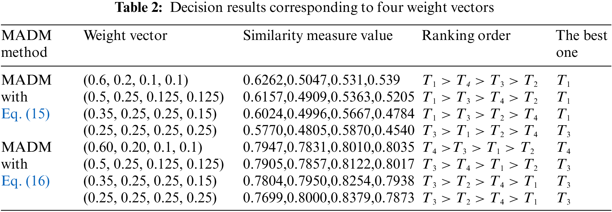
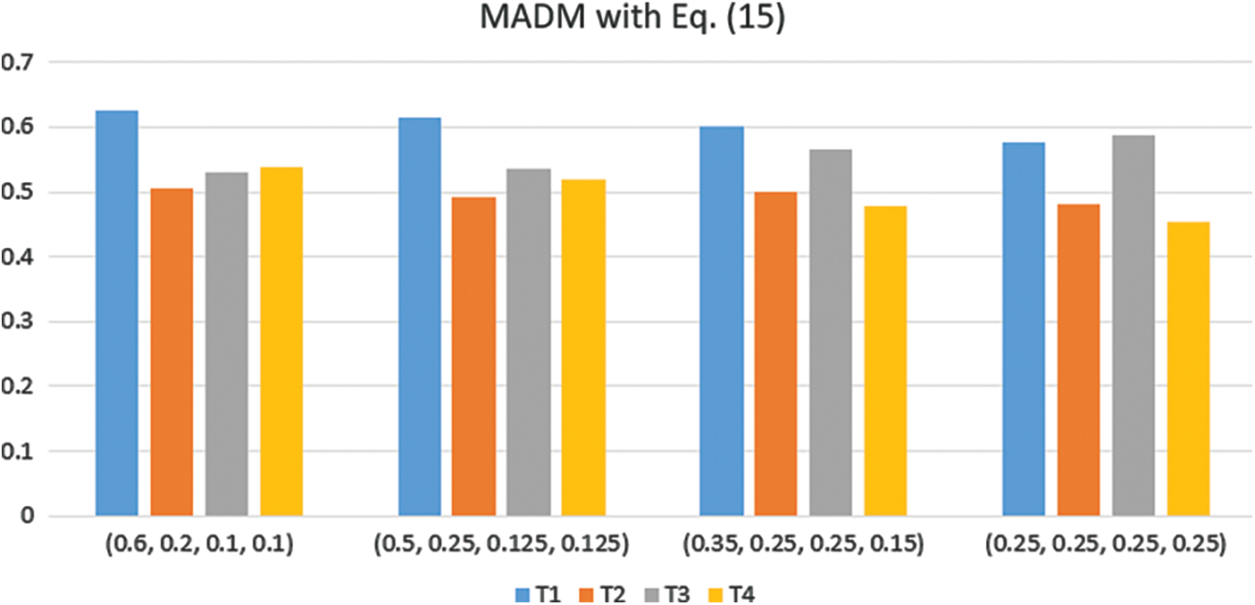
Figure 1: MADM with Eq. (15)
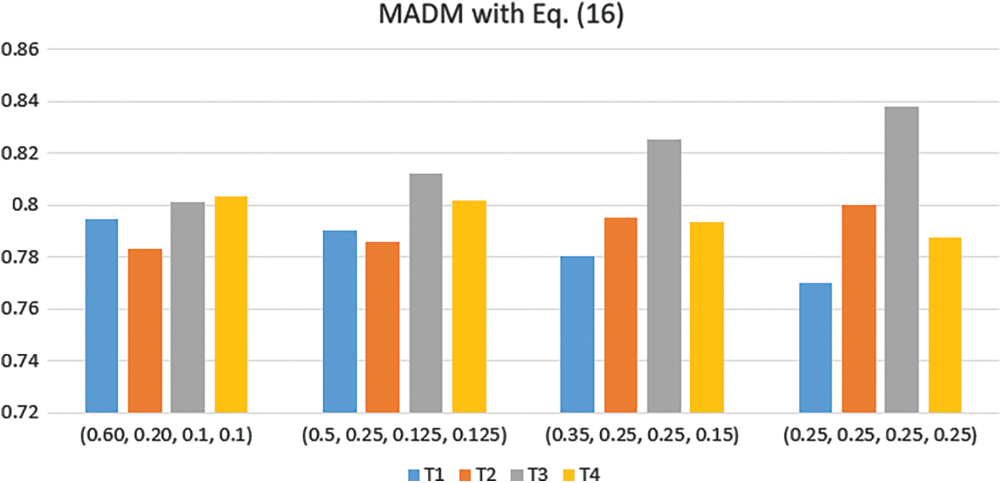
Figure 2: MADM with Eq. (16)
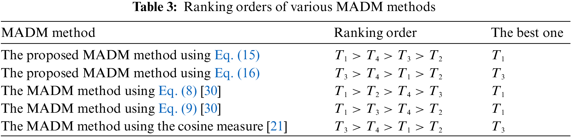
In this section, the proposed MADM approach based on the cotangent similarity measures is compared with the MADM method in [21,30] to prove the feasibility and effectiveness of the proposed MADM method.
To enhance the comparability, we use the same weight vector w = (0.5, 0.25, 0.125, 0.125) for various MADM methods and present their decision results in Table 3. In Table 3, the ranking order of the proposed MADM approach using Eq. (15) is mostly consistent with the MADM method using Eq. (9) [30]. Two Eqs. (15) and (9) [30] using the parameter ‘max’, which has the same result. It shows that the results are reasonable. Then, the ranking order of the MADM method proposed by Eq. (16) is calculated with the average, which is the same as the MADM method using the cosine measure [21]. The comparison results show the efficiency of the proposed MADM approach. However, the MADM method using the cosine measure [21] does not consider the consistent degree in the MADM process, which may lead to the loss of some useful information and the difference in sorting results. Furthermore, the consistent degree of multi-valued sequences can affect the sorting results of alternatives, revealing the importance of the consistent information in MADM problems, and making the decision results more credible and reasonable.
The advantages of the cotangent similarity measure in this study can make up for some deficiencies of the cosine similarity measure in the vector space to a certain extent. Using two different methods of cotangent similarity measures, different ranking results can be obtained. It shows that the results have excellent plasticity and rationality. At the same time, the method also provides a new way of thinking about the multi-valued decision-making problem.
Based on the concepts of NMVS and CSVNSs, the cotangent similarity measures of CSVNSs are proposed by the cotangent function. The proposed MADM method using the cotangent similarity measures of CSVNSs is applied to perform the MADM problem with NMVSs. Then, the proposed MADM method is applied to the selection problem of potential cars to verify the effectiveness of the proposed MADM method. Compared with other MADM methods, the proposed MADM method shows its high efficiency and rationality. In future research, we will further develop other new similarity measures of CSVNSs and apply them in the fields of medical diagnosis/ assessment and image processing in the setting of NMVSs.
Funding Statement: The authors received no specific funding for this study.
Conflicts of Interest: The authors declare that they have no conflicts of interest to report on the present study.
References
1. Zadeh, L. A. (1965). Fuzzy sets. Information and Control, 8(3), 338–353. DOI 10.1016/S0019-9958(65)90241-X. [Google Scholar] [CrossRef]
2. Atanassow, K. (1986). Intuitionistic fuzzy sets. Fuzzy Sets and Systems, 20(1), 87–96. DOI 10.1016/S0165-0114(86)80034-3. [Google Scholar] [CrossRef]
3. Smarandache, F. (1998). Neutrosophy: Neutrosophic probability, set, and logic. Rehoboth, DE, USA: American Research Press. [Google Scholar]
4. Anter, A. M., Hassanien, A. E., Elsoud, M. A. A., Tolba, M. F. (2014). Neutrosophic sets and fuzzy c-means clustering for improving CT liver image segmentation. Advances in Intelligent Systems and Computing, 303, 193–203. DOI 10.1007/978-3-319-08156-4. [Google Scholar] [CrossRef]
5. Guo, Y., Xia, R., Şengür, A., Polat, K. (2017). A novel image segmentation approach based on neutrosophic c-means clustering and indeterminacy filtering. Neural Computing and Applications, 28(10), 3009–3019. DOI 10.1007/s00521-016-2441-2. [Google Scholar] [CrossRef]
6. Ma, Y. X., Wang, J. Q., Wang, J., Wu, X. H. (2017). An interval neutrosophic linguistic multi-criteria group decision-making method and its application in selecting medical treatment options. Neural Computing and Applications, 28(9), 2745–2765. DOI 10.1007/s00521-016-2203-1. [Google Scholar] [CrossRef]
7. Guo, Y., Sengur, A. (2015). NECM: Neutrosophic evidential c-means clustering algorithm. Neural Computing and Applications, 26(3), 561–571. DOI 10.1007/s00521-014-1648-3. [Google Scholar] [CrossRef]
8. Wang, H., Smarandache, F., Sunderraman, R. (2010). Single valued neutrosophic sets. Multispace and Multistructure, 4, 410–413. [Google Scholar]
9. Ye, J., Zhang, Q. S. (2014). Single valued neutrosophic similarity measures for multiple attribute decision making. Neutrosophic Sets and Systems, 2, 48–54. [Google Scholar]
10. Rahman, A. U., Saeed, M., Alodhaibi, S. S., Khalifa, H. A. E. (2021). Decision making algorithmic approaches based on parameterization of neutrosophic set under hypersoft set environment with fuzzy, intuitionistic fuzzy and neutrosophic settings. Computer Modeling in Engineering & Sciences, 128(2), 743–777. DOI 10.32604/cmes.2021.016736. [Google Scholar] [CrossRef]
11. Ye, J. (2014). Clustering methods using distance-based similarity measures of single-valued neutrosophic sets. Journal of Intelligent Systems, 23(4), 379–389. DOI 10.1515/jisys-2013-0091. [Google Scholar] [CrossRef]
12. Ye, J. (2014). Single valued neutrosophic cross-entropy for multicriteria decision making problems. Applied Mathematical Modelling, 38(3), 1170–1175. DOI 10.1016/j.apm.2013.07.020. [Google Scholar] [CrossRef]
13. Hu, K., Ye, J., Fan, E., Pi, J. (2017). A novel object tracking algorithm by fusing color and depth information based on single-valued neutrosophic cross-entropy. Journal of Intelligent & Fuzzy Systems, 32(3), 1775–1786. DOI 10.3233/JIFS-152381. [Google Scholar] [CrossRef]
14. Liu, P. D. (2016). The aggregation operators based on Archimedean t-conorm and t-norm for single-valued neutrosophic numbers and their application to decision making. Journal of Intelligent & Fuzzy Systems, 18(5), 1–15. DOI 10.1007/s40815-016-0195-8. [Google Scholar] [CrossRef]
15. Zeng, S., Luo, D., Zhang, C., Li, X. (2020). A correlation-based TOPSIS method for multiple attribute decision making with single-valued neutrosophic information. International Journal of Information Technology & Decision Making, 19(1), 343–358. DOI 10.1142/S0219622019500512. [Google Scholar] [CrossRef]
16. Ye, J. (2014). A multicriteria decision-making method using aggregation operators for simplified neutrosophic sets. Journal of Intelligent & Fuzzy Systems, 26(5), 2459–2466. DOI 10.3233/IFS-130916. [Google Scholar] [CrossRef]
17. Wu, X. H., Wang, J. Q., Peng, J. J., Chen, X. H. (2016). Cross-entropy and prioritized aggregation operators with simplified neutrosophic sets and their application in multi-criteria decision-making problems. International Journal of Fuzzy Systems, 18(6), 1104–1116. DOI 10.1007/s40815-016-0180-2. [Google Scholar] [CrossRef]
18. Zhou, L. P., Dong, J. Y., Wan, S. P. (2019). Two new approaches for multi-attribute group decision-making with interval-valued neutrosophic frank aggregation operators and incomplete weights. IEEE Access, 7(1), 102727–102750. DOI 10.1109/ACCESS.2019.2927133. [Google Scholar] [CrossRef]
19. Tu, A., Ye, J., Wang, B. (2018). Symmetry measures of simplified neutrosophic sets for multiple attribute decision-making problems. Symmetry, 10(5), 144. DOI 10.3390/sym10050144. [Google Scholar] [CrossRef]
20. Ye, S., Ye, J. (2014). Dice similarity measure between single valued neutrosophic multisets and its application in medical diagnosis. Neutrosophic Sets and Systems, 6, 49–54. [Google Scholar]
21. Fan, C., Fan, E., Ye, J. (2018). The cosine measure of single-valued neutrosophic multisets for multiple attribute decision-making. Symmetry, 10(5), 154. DOI 10.3390/sym10050154. [Google Scholar] [CrossRef]
22. Ye, J. (2015). Multiple-attribute decision-making method under a single-valued neutrosophic hesitant fuzzy environment. Journal of Intelligent Systems, 24(1), 23–36. DOI 10.1515/jisys-2014-0001. [Google Scholar] [CrossRef]
23. Wang, J. Q., Li, X. (2015). TODIM method on multi-valued neutrosophic sets. Control and Decision, 30(6), 1139–1142. [Google Scholar]
24. Peng, J. J., Wang, J. Q., Wu, X. H., Chen, X. H. (2015). Multi-valued neutrosophic sets and power aggregation operators with their applications in multi-criteria group decision-making problems. International Journal of Computing Intelligent Systems, 8(2), 345–363. DOI 10.1080/18756891.2015.1001957. [Google Scholar] [CrossRef]
25. Peng, J. J., Wang, J. Q., Yang, W. E. (2017). A multi-valued neutrosophic qualitative flexible approach based on likelihood for multi-criteria decision-making problems. International Journal of Systems Science, 48(2), 425–435. DOI 10.1080/00207721.2016.1218975. [Google Scholar] [CrossRef]
26. Peng, J. J., Wang, J. Q., Wu, X. H. (2017). An extension of the electre approach with multi-valued neutrosophic information. Neural Computing and Applications, 28(S1), 1011–1022. DOI 10.1007/s00521-016-2411-8. [Google Scholar] [CrossRef]
27. Ji, P., Zhang, H. Y., Wang, J. Q. (2018). A projection-based TODIM method under multi-valued neutrosophic environments and its application in personnel selection. Neural Computing and Applications, 29(1), 221–234. DOI 10.1007/s00521-016-2436-z. [Google Scholar] [CrossRef]
28. Peng, J. J., Tian, C. (2018). Multi-valued neutrosophic distance-based QUALIFLEX method for treatment selection. Information, 9(12), 327. DOI 10.3390/info9120327. [Google Scholar] [CrossRef]
29. Xu, D., Peng, L. (2021). An improved method based on TODIM and TOPSIS for multi-attribute decision-making with multi-valued neutrosophic sets. Computer Modeling in Engineering & Sciences, 129(2), 907–926. DOI 10.32604/cmes.2021.016720. [Google Scholar] [CrossRef]
30. Ye, J., Song, J., Du, S. (2021). Correlation coefficients of consistency neutrosophic sets regarding neutrosophic multi-valued sets and their multi-attribute decision-making method. International Journal of Fuzzy Systems, 24(2), 925–932. DOI 10.1007/s40815-020-00983-x. [Google Scholar] [CrossRef]
 | This work is licensed under a Creative Commons Attribution 4.0 International License, which permits unrestricted use, distribution, and reproduction in any medium, provided the original work is properly cited. |