| Computer Modeling in Engineering & Sciences |
DOI: 10.32604/cmes.2022.020738
ARTICLE
A CFD-DEM-Wear Coupling Method for Stone Chip Resistance of Automotive Coatings with a Rigid Connection Particle Method for Non-Spherical Particles
1School of Mechanical & Automotive Engineering, South China University of Technology, Guangzhou, 510641, China
2School of Marine Engineering and Technology, Sun Yat-sen University, Zhuhai, 510275, China
3Southern Marine Science and Engineering Guangdong Laboratory (Zhuhai), Zhuhai, 528315, China
4RIKEN Center for Computational Science, Kobe, 650-0047, Japan
*Corresponding Authors: Mengyan Zang. Email: myzang@scut.edu.cn; Shunhua Chen. Email: chenshh73@mail.sysu.edu.cn
Received: 09 December 2021; Accepted: 22 February 2022
Abstract: The stone chip resistance performance of automotive coatings has attracted increasing attention in academic and industrial communities. Even though traditional gravelometer tests can be used to evaluate stone chip resistance of automotive coatings, such experiment-based methods suffer from poor repeatability and high cost. The main purpose of this work is to develop a CFD-DEM-wear coupling method to accurately and efficiently simulate stone chip behavior of automotive coatings in a gravelometer test. To achieve this end, an approach coupling an unresolved computational fluid dynamics (CFD) method and a discrete element method (DEM) are employed to account for interactions between fluids and large particles. In order to accurately describe large particles, a rigid connection particle method is proposed. In doing so, each actual non-spherical particle can be approximately described by rigidly connecting a group of non-overlapping spheres, and particle-fluid interactions are simulated based on each component sphere. An erosion wear model is used to calculate the impact damage of coatings based on particle-coating interactions. Single spherical particle tests are performed to demonstrate the feasibility of the proposed rigid connection particle method under various air pressure conditions. Then, the developed CFD-DEM-wear model is applied to reproduce the stone chip behavior of two standard tests, i.e., DIN 55996-1 and SAE-J400-2002 tests. Numerical results are found to be in good agreement with experimental data, which demonstrates the capacity of our developed method in stone chip resistance evaluation. Finally, parametric studies are conducted to numerically investigate the influences of initial velocity and test panel orientation on impact damage of automotive coatings.
Keywords: Automotive coating; stone chip resistance; gravelometer; non-spherical particle; composite particle; CFD-DEM
Nomenclature
| Particle impact angle | |
| Volume fraction occupied by the fluid | |
| Position vector from the particle's center to the contact point | |
| Drag force coefficient | |
| Diameter of the component sphere | |
| Volume-equivalent diameter of the original particle | |
| Overlap distance of two particles in contact | |
| Tangential displacement vector between the two particles in contact | |
| Coefficient of restitution | |
| Eroded mass | |
| Particle-wall contact force | |
| Particle-particle and particle-wall contact forces | |
| Particle-wall contact forces | |
| Fluid-particle interaction force | |
| Bonding force | |
| Resultant force of rigid composite particle | |
| Resultant force of component sphere i | |
| Normal contact force between particle i and particle j | |
| Tangential contact force between particle i and particle j | |
| Drag force | |
| Buoyancy force | |
| Resultant force after bonded | |
| Acceleration of gravity | |
| Equivalent shear modulus | |
| Moment of inertia of the composite particle | |
| Normal elastic constant | |
| Tangential elastic constant | |
| Equivalent mass | |
| Mass of the component sphere i | |
| Mass of the composite particle | |
| Resultant moment on the mass center of rigid composite particle | |
| Number of component sphere in the composite particle | |
| Fluid density | |
| Particle density | |
| Air flow rate | |
| Position vector from the center of mass of the composite particle to the component sphere i | |
| Particle Reynolds number | |
| Momentum exchange with the particulate phase | |
| Radius of particle i | |
| Equivalent radius | |
| Impingement angle | |
| Normal viscoelastic damping constant | |
| Tangential viscoelastic damping constant | |
| Normal stiffness | |
| Tangential stiffness | |
| Contact time | |
| Stress tensor for the fluid phase | |
| Fluid velocity | |
| Particle velocity | |
| Fluid dynamic viscosity | |
| Poisson's ratio of particle i | |
| Initial velocity of particles | |
| Relative velocity of the particle i and particle j in contact | |
| Particle impact velocity | |
| Stable gas velocity | |
| Inlet velocity | |
| Fluid kinematic viscosity | |
| Young's Modulus of particle i | |
| Equivalent Young's Modulus |
Automotive coating plays an important role in providing resistance to corrosion, rusting, stone impact and aging for vehicle surface. However, the possible damage of coating caused by flying debris during high-speed driving could do harm to a vehicle in terms of appearance and safety. Since the anti-impact capability of automotive coating has always been highly concerned by vehicle companies and users, it is of great significance to find an effective and accurate method to evaluate the stone chip resistance of the surface coating. At present, automobile companies usually adopt tests according to standards, e.g., DIN 55996-1 and SAE J400-2002, to evaluate the stone chipping resistance of the coating. Although test evaluation has the advantages of intuition and reliability, it is of high cost, low efficiency and poor repeatability. Evaluation by computer simulation can parameterize the research and overcome the deficiency of experiment. Besides, the simulation results can also serve to guide the test, which significantly shortens the development cycle.
The standardized tests are often performed on a gravel projecting test apparatus, which is named gravelometer in standard SAE J400-2002. In order to accurately and efficiently reproduce the movement of particles in the experiment and obtain reliable impact velocity and impact position for wear model by simulation, the widely accepted coupled CFD-DEM method (unresolved CFD-DEM) is employed in this study. Attributed to its excellent computational efficiency and the capability to trace the particle motion, the unresolved CFD-DEM method is widely used in particulate flow simulations such as pneumatic conveying, fluidized bed and blast furnace [1]. Related researches have proven that this method has the capability to reproduce complicated flow regimes and particle motions in pipelines [2,3]. In addition, combined with a wear model, the unresolved CFD-DEM method has been confirmed to have the capability to predict the particle-induced erosion [2], which is promising for the application on the automotive coating. For instance, Zhao et al. [4] and Tang et al. [5] studied the erosion in a centrifugal pump during non-spherical particle transportation. By similar means, Nguyen et al. [6] investigated the effect of impinging angle, sand particle flux and impinging velocity on the erosion rate and erosion pattern of a specimen surface.
Nevertheless, the conventional unresolved CFD-DEM method has its limitations. The first limitation is the difficulty of non-spherical particle representation, which is of great necessity in this study as is demanded in the corresponding standardized tests. However, the models implemented in the conventional unresolved CFD-DEM method are mostly developed for spherical particles, which means both DEM approaches and CFD-DEM coupling strategies need to be further redeveloped for non-spherical particles [7]. So far, a number of researchers have been devoted to developing proper presentation method for non-spherical particles to reproduce non-spherical granular flows. For cases where the particle's shape representation and contact do not play a major role in its movement, the non-spherical particles can be substituted by spherical particles that have equivalent diameters and shape factors [8–10]. Factors such as sphericity [11,12], roundness [13], circularity [14] are used as an implementation of the drag coefficient. Relevant experimental researches are needed to determine the particle's movement pattern under different circumstances, and a drag coefficient correlation can be formulated considering the effect of the particle shape and possibly the particle moving orientation [15,16]. This method is easy to implement and has the capability to accurately simulate particle translation such as particle settlement, but the particle rotation is predicted with lower accuracy. For other cases where the particle shape representation is considered necessary, analytical models, e.g., ellipsoids, cylinders, super-quadrics and polyhedrons, were developed to present complex shapes within discrete element method [17]. In addition to the drag coefficient correlation mentioned above, new particle representation model and contact model are required for the particle-particle and particle-wall contact detection as well as contact force computation [18]. This method can be quite detailed and realistic in describing particle motion of a specific shape, and has higher computational efficiency compared with methods of the same precision [19], which is more suitable for industrial applications. Podlozhnyuk et al. [20] modeled several particle shapes by super-quadric model and applied them to cases such as angle of repose measurement and hopper/silo discharge, which showed promising results qualitatively and quantitatively. But this method also has high development difficulty in handling contact detection and it is hard to deal with the occasions where there exist a variety of non-spherical particles.
The most popular approach to define non-spherical particle is the composite particle method, in which several component spheres are bonded together for shape approximation. The composite spheres method is excellent in its simplicity and unrestricted shape representation [17]. It is easy to implement because the established framework of spherical DEM can be directly applied to component spheres of the composite particles. The accuracy of particle shape representation and inter-particle contact computation increases with the component sphere number in an individual composite particle [21], but so does the computational cost. As a result, most researches on composite particle try to use as few spheres as possible to create non-spherical particle considering computational efficiency [22].
The composite particle model with component spheres overlapping is broadly used to form non-spherical particles in granular flows. Li et al. [23] studied the particulate flow in the air-blowing seed metering device adopting overlapping composite particles to represent the shape of the soybean seed. Ren et al. [24] investigated the spouting action of corn-shaped particles in a cylindrical spouted bed. The corn-shaped particles are composed of overlapping spheres and the contact pattern was further illustrated. Nevertheless, when coupled with fluid, the large overlapping between spheres increases the difficulty of the computation of void fraction and affects the accuracy of inter-phase interaction force calculation. The non-overlapping composite particles are mainly used in CFD-DEM simulations to address the issue described above. By using the bonded particle method (BPM), Jensen et al. [25] arranged the particles into a line without overlapping to approximate the shape of the flexible fiber. The flexibility of particles was well presented by the BPM method, and the predicted drag coefficient was in good agreement with the experimental one. Guo et al. [26] adopted glued-sphere particles and true cylinder particles to study the influence of particle shape on the granular flow behavior. Similarly, Sun et al. [22] bonded a few particles without overlapping together to represent a series of sediment grain shapes in simulation. The fluid-particle interaction force is computed and applied on every component sphere, which shows better performance in representing the fluid-exerted torque on the composite particles. Therefore, for the complex situations in this study where multiple non-spherical particles are involved, the composite particle method has high application value.
The second limitation is the mesh-particle size ratio. For the unresolved CFD-DEM method, by solving the locally averaged Navier-Stokes equation, the flow around each particle is volume-averaged in the local domain [27]. To ensure the accuracy and astringency of the computation, the size of the mesh should at least be 3 times as large as the size of particles [28,29]. But in stone chip resistance tests, in order to obtain a stable and sufficient acceleration effect, the size of selected projectiles is often not much smaller than the diameter of accelerating pipe. In this case, if the requirement of mesh-particle size ratio is met, the fluid mesh will be too coarse to get convergent results. To overcome this “large particle” limitation, there are basically two approaches. One is to use the resolved CFD-DEM method (DNS-DEM) as a substitute to handle the coupling. The difference between the “resolved” and “unresolved” CFD-DEM method is whether the particles and the flow around them are resolved in the fluid field. Different from the unresolved CFD-DEM method where the detailed flow around each individual particle is locally averaged, the resolved CFD-DEM method has the capability to capture particle boundaries and the fluid flow around each particle precisely [30]. A semi-resolved CFD-DEM method proposed by Cheng et al. [31] combines the unresolved and the resolved CFD-DEM method to deal with situations where coarse particles and fine particles coexist. It overcomes the contradiction between the requirements of different particle sizes for the mesh size and the computational difficulty of large particle motion in the flow field. However, to keep the results accurate and precise, the resolved CFD-DEM method requires the particle diameter to be 10 times more than the mesh size, which leads to a large-scale model and heavy computational burden [29,32]. Moreover, in high Reynolds number conditions, the mesh around particles should be finer in order to resolve the boundary layer, which further increases computational cost [33].
The other method is to improve the void fraction model on the basis of the unresolved CFD-DEM method. At present, the most broadly used void fraction models in the unresolved CFD-DEM method are the particle centroid method (PCM) and the divided particle volume method (DVPM) [34]. The PCM simply attributes the entire volume of a particle to the cell where the ball center is located, while The DVPM searches for all the particles overlap with the targeted cell, calculates and sums up the overlap volume to compute the void fraction. These two methods are considered accurate when the mesh size is much larger than the particle size, but error increases when the mesh size is close to or smaller than the particle size. In extreme cases, the local extremes of void fraction of the cells around particle centroid may reach or exceed 100%, which means the cell is fully occupied by particles. Continuity equation are very likely to diverge in this situation. And that is the essence of “large particle” limitation. Related researches have been conducted by many researchers. Link et al. [35] proposed a porous cube method to calculate the void fraction. In this method, the volume of every single sphere is evenly distributed to a cubic space, which is several times larger than the particle and centered on the ball center, to smooth void fraction and avoid local extremes of void fraction in the cells around particle centroid. Then the void fraction of several cubic spaces will be mapped to actual void fraction field. Similarly, Jing et al. [36] replaced the cubic space in the porous cube method with a spherical space and put forward a porous sphere void fraction model to simulate particle sedimentation. Xiao et al. [37] introduced a distance-dependent weighting function into the porous sphere method, further optimizing the calculation from particle volume distribution. Volume of a certain particle is distributed to all the cells within a specified cutoff distance, which is based on a Gaussian function and the distance from the cell center to the particle centroid. It shows better performance in reproducing the influence of particles upon flow field than the volume averaging strategy. Likewise, Yang et al. [38], Zhu et al. [39] introduced respectively a Gaussian function and a double cosine kernel function (SCKF) into the semi-resolved method as the void fraction distribution function to handle the coarse particles.
Taking the aforementioned limitations into account, Xiong et al. [40] bonded quantities of particles together to form a large particle of irregular shape based on the bonded particle method (BPM). The particles do not overlap, giving rise to a physically-porous composite particle. The fluid forces are calculated on each small particle. The method was compared with the immersed boundary method (IBM) through single particle sedimentation simulation. The computation results showed that with a similar accuracy, the BPM has obvious advantages over the IBM in terms of computational efficiency, especially when large quantities of particles are situated in the computational domain. However, after collision, the bonded particles are likely to deform or even break down due to bond breakage, making the simulation unstable. Moreover, the additional degrees of freedom of the component spheres which belongs to the same composite particle unnecessarily increases computational cost.
In this work, the rigid connection particle method is proposed to address the issues of the bonded particle method mentioned above. While the unresolved CFD-DEM method is still adopted to describe the gas-particle two-phase flow field, the adhesive bond connections between particles in the bonded particle method is replaced by rigid connections to form composite particles. This method uses hundreds of and possibly thousands of non-overlapping spheres to approximately represent the shape of the original particle. The sphere cluster is treated as a rigid body. According to the resultant external force and position of each component sphere, the resultant force and moment of the rigid composite particle is computed, which is then used to solve the motion of the rigid composite particle. The proposed method combines the composite sphere method with the idea of the porous sphere method. It replaces the original particles with non-overlapping composite particles to realize the porous structure. On the one hand, particles of any shape can be represented using the composite particle method. On the other hand, the local extremes of void fraction around particle centroid can also be avoided, attributed to the porous structure. Moreover, by controlling the diameter of component spheres, the requirement of mesh-particle size ratio can be met to keep the numerical results accurate and convergent. As a consequence, it can cope well with the simulations of DIN and SAE tests. Moreover, as an optimization of the BPM, the proposed method has better performance in reproducing the particle rotation and is free from the concerns of bond breakage.
This paper is organized as follows. In Section 2, the governing equations of the unresolved CFD-DEM method and the newly proposed method for handling large particles are introduced. In Section 3, we perform single spherical particle motion simulations with the rigid connection particle method. The competence of the method under high-Reynolds number conditions is demonstrated by comparing the numerical results with the experimental outcomes as well as that predicted by using the bonded particle method. In Section 4, coupled with wear model originally proposed by Finnie [41], the proposed method is applied to DIN standard and SAE standard multi-particle simulation, and the results are compared with experiments in terms of particle impact velocity and impact damage distribution. The influences of average impact velocity and test panel orientation on coating damage are then numerically studied, which proves the validity and accuracy of the proposed method in evaluating the coating resistance towards the stone chipping. Finally, Conclusion of this study is drawn in Section 5.
The unresolved CFD-DEM method employed in this study is founded on the Euler-Lagrangian framework [42]. The fluid, which is air in this study, is regarded as a continuous phase based on the Euler method, and the locally averaged characteristics of fluid are accounted for by using the finite volume method. The standard k-ε model is applied to the simulations in this study. Solid particles are regarded as a discrete phase based on the Lagrangian method. The translational and rotational motions for each composite particle are updated based on the discrete element method. The interaction of fluid and particle is realized in the form of momentum exchange. In this section, the equations for the rigid connection particle method are at first introduced, and the equations describing the fluid flows, the fluid-particle interaction as well as the particle-induced wear are then presented. At last, the structure of the unresolved CFD-DEM method is briefly introduced.
2.1 Rigid Connection Particle Method Based on DEM
In this study, a novel method called rigid connection particle method is proposed to handle large particles in a narrow channel. A group of spheres are rigidly connected to form a rigid composite particle of arbitrary shape, and some instances are shown in Fig. 1. In this way, the actual particle size is reduced and flow field mesh's restrictions on particle size are relaxed.

Figure 1: Some instances of rigid composite particle
A rigid composite particle usually consists of hundreds of component spheres which do not overlap and fit tightly. It was pointed out in previous studies that the size of the mesh should at least be 3 times as large as the size of particles to ensure the accuracy and astringency of the computation [28,29]. In order to minimize the number of component sphere contained in a large particle and improve computational efficiency, the radii of component spheres are all set to be 1/3 of the minimum cell size. Derived from the DEM, the translational and rotational movements of rigid composite particles are calculated based on Newton's second law of motion [43,44]:
where
Although the appearance of the rigid composite particle is similar to that of the bonded composite particle proposed by Xiong et al. [40], there is a big difference between these two methods in numerical implementation. The principles of these two methods are displayed and compared in Fig. 2. The bonded particle method assumes that the particles are connected via spring-dashpot systems in the tangential and normal directions. The bonding force between particles keeps the component particles moving as a whole, and the movement of each sphere is computed individually. Since this method does not calculate the moment of composite particle, the representation of the particle rotation will be much less accurate. Also, the additional degrees of freedom of the component spheres which belongs to the same composite particle increases the force and speed fluctuations.

Figure 2: The comparison of numerical implementation between the two methods (F1, F2: original resultant force before connected; Fb: bonding force; Ft: resultant force after bonded; Fc, Mc: resultant force and moment on the mass center of rigid composite particle)
In comparison, the rigid connection particle method fixes the relative position of the two spheres and treats them as a whole, transforming the forces on sphere to the forces and moments on the center of mass of the composite particle, which has better performance in describing particle movement. As shown in Fig. 3, two non-spherical composite particles, which are identical except for the connection method, collides with a wall and bounces under the same conditions. Usually, when a particle collides with a wall, the tangential contact force will produce a torque which rotates the particle. The rigid composite particle can reproduce the rotation while the bonded particle almost keeps its orientation unchanged. Besides, the proposed method can use longer time step without the occurrence of bond breakage and unphysical oscillations, which is conducive to improving computational efficiency.

Figure 3: Particle trajectory after collision (a) the bonded particle method (b) the rigid connection particle method
2.2 Locally Averaged Navier–Stokes Equations for Fluid Flows
The fluid phase is assumed to be incompressible in order to simplify the simulation model. It is governed by the corresponding locally averaged Navier-Stokes equations [27]:
where
2.3 Contact Model for Solid Phase
The particle-wall contact and particle-particle contact are computed based on the Hertz-Mindlin no-slip contact model [45,46] and a soft-sphere model proposed by Cundall et al. [43]. This model treats component spheres as soft spheres, and allows small overlap between particles and between particles and walls. An example of particle-particle contact is shown in Fig. 4a. When two composite particles get close enough, a component sphere on composite particle A will overlap with a component sphere on composite particle B. The normal and tangential contact forces are computed based on a non-linear spring-dashpot contact model, as shown in Figs. 4b, 4c. The equations of the normal contact force
where

Figure 4: The spring-dashpot contact model (a) The definition of the overlap distance (b) normal contact force (c) tangential contact force
Further, the normal and tangential elastic constant as well as viscoelastic damping constant are computed as [47]:
where
The equivalent Young's Modulus, equivalent shear modulus, equivalent radius, equivalent mass are defined as:
where
2.4 Fluid-Particle Interaction
In the unresolved CFD-DEM method, the interaction force between the fluid and particle is generally calculated by an empirical formula determined via experiments. In this study, the drag force
where
where
Moreover, Kodam et al. [50] concluded that although the use of more component spheres in a composite particle could improve the accuracy of geometrical shape representation, it can lead to a reduced accuracy in force modeling. Because of the porousness of the composite particle in this work, part of the flow which should have gone around the particle travels through it instead, which causes errors in the computation of drag force. To reproduce the particle movement, the averaged fluid velocity of all the girds overlapped with the certain composite particle is calculated as the background velocity. A new coordinate system is created with the direction of the background velocity as the X’ axis and the Y’ axis parallel to the original XY plane, as shown in Fig. 5.

Figure 5: Definition of the background fluid velocity
Subsequently, a parameter K dependent on the composite particle characteristics is used as a multiplier to scale the drag force component
where D is the volume-equivalent diameter of the original spherical or non-spherical particle; dp is the diameter of component sphere; Ns is the number of spheres in a single composite particle.
The coating damage is predicted by using the erosion wear model proposed by Finnie [41] in simulation. The rate of wear is calculated on the basis of the rate of kinetic energy:
where k is a constant;
The eroded mass (EM) during contact time can be computed as:
where
2.6 The Unresolved CFD-DEM Algorithm
In this paper, the proposed method and the unresolved CFD-DEM method are implemented in CFDEM®coupling framework [51]. As shown in Fig. 6, the two-way coupling of the open source CFD solver, i.e., OpenFOAM [52], and DEM solver, i.e., LIGGGHTS [53], is realized via the CFDEM coupling interface. Generally, the CFD time step is set to be an integer multiple of the DEM time step to save computational cost, and the integer is chosen as 10 in this paper. The coupling computation in a CFD time step is performed in the following way. At first, the flow field data calculated in the last time step is transferred to the coupling interface. Combined with all the particle information fetched by the coupling interface, the void fraction field and the interaction force for each sphere are computed. After that, the interaction force is transferred to the DEM part as an external force acting on component sphere. The DEM solver is then triggered and the translation and rotational motions of composite particles are computed on the basis of the rigid connection particle method. Next, the positions of the component spheres are updated. The panel erosion caused by particle-wall contact is also computed. Another 9 DEM time steps will then be computed before the interaction force and void fraction field being transferred to the CFD part. Finally, the Navier-Stokes equations are solved for the next CFD time step.

Figure 6: Structure of the unresolved CFD-DEM algorithm
Currently, most researches on large particles focus on low Reynolds number conditions. In order to verify the feasibility of the proposed method under the situations of high Reynolds number, single particle motion tests were carried out on the stone chip resistance gravelometer, and the corresponding simulation is performed in our study. The structure of the gravelometer used in this research is shown schematically in Fig. 7. In order to adapt to different standards and research needs, the output air pressure, the orientation of test panel, as well as the size of the accelerating pipe can be adjusted. For multi-particle test, a certain amount of gravel is thrown into the feed inlet, falls uniformly under vibration, moves through the pipe driven by high-speed air flow and impacts the test panel. But in order to ensure the repeatability of single particle motion tests, instead of being put in through the vibrating feeder during test, a 5 mm diameter steel ball is placed in the DIN standard accelerating pipe in advance with its initial position determined. When the test begins, the steel ball moves through the pipe under the drive of high-speed air flow with its trajectory captured by a high-speed camera. The particle velocity can be calculated from the displacement between two consecutive frames in the video.

Figure 7: Schematic of the structure of gravelometer (Decompression components and measurement components are omitted)
Five single particle tests S1 to S5, with air pressures setting ranging from 0.05 MPa to 0.25 MPa, were used to verify the applicability of the proposed approach in a variety of high Reynolds number conditions. Simulations are conducted in both the rigid connection particle method and the bonded particle method according to the experimental conditions to compare their computational efficiency and accuracy. The simulations focus on the motion of particle inside the DIN accelerating pipe, and the computational domain is set to be a horizontal circular pipe with a length of 290 mm and an inner diameter of 30 mm. Its schematic diagram and related dimensions and parameters are shown in Fig. 8. Parameters for different cases are displayed in Table 1.

Figure 8: Schematic diagram of the single particle simulation

Simulation parameters are set according to experimental conditions, with the stable gas velocity
The outlet is set as a pressure outlet, with the fixed pressure value set as 0. No-slip boundary condition is applied on the wall of the pipe. The 5 mm diameter spherical composite particle is made up of 615 component spheres with a diameter of 0.5 mm, and is placed in the corresponding position of the steel ball in the experiment. The composite particle used in the rigid connection particle method and the bonded particle method are identical except for the way the component spheres are connected. Other parameters for fluid and particles are displayed in Table 2. Parameters for the bonded particles are set to be the same with Xiong et al. [40]. For brevity, they are not presented in this paper.

Fig. 9 compares the predicted histories of horizontal particle displacement with the experimental outcomes. The solid line and the dashed line represent the simulated results using the rigid connection particle method and bonded particle method respectively, and the scattered point represents the experimental results. As shown in the graph, along the horizontal direction of the computational domain, the particle starts to move from rest driven by high-speed airflow, with its horizontal velocity increasing continuously until the particle leaves the computational domain. The particle horizontal velocity at the outlet increases with the increase of set air pressure. The simulation results of the both methods are in great agreement with the experimental results, but the results of the rigid connection particle method have smaller discrepancy in higher air pressure conditions.

Figure 9: The particle displacement in x direction (R and B represent the simulation results of the rigid connection particle method and bonded particle method, E represent the experimental results)
In the vertical direction, it is hard to capture the particle movement accurately since the movement amplitude is not large enough for the high-speed camera and corresponding post-processing software. Given the above, the results are described with the maximum height the particle reaches and the number of particle collisions against the pipe wall. The data is displayed in Table 3. The particles are at first lifted by the high-speed air flow, and fall under the influence of gravity, back and forth, colliding with the pipe wall several times. The experimental and numerical results show similar trend that the higher the air pressure is set, the greater the amplitude of particle uplift and the fewer collisions with the pipe wall.
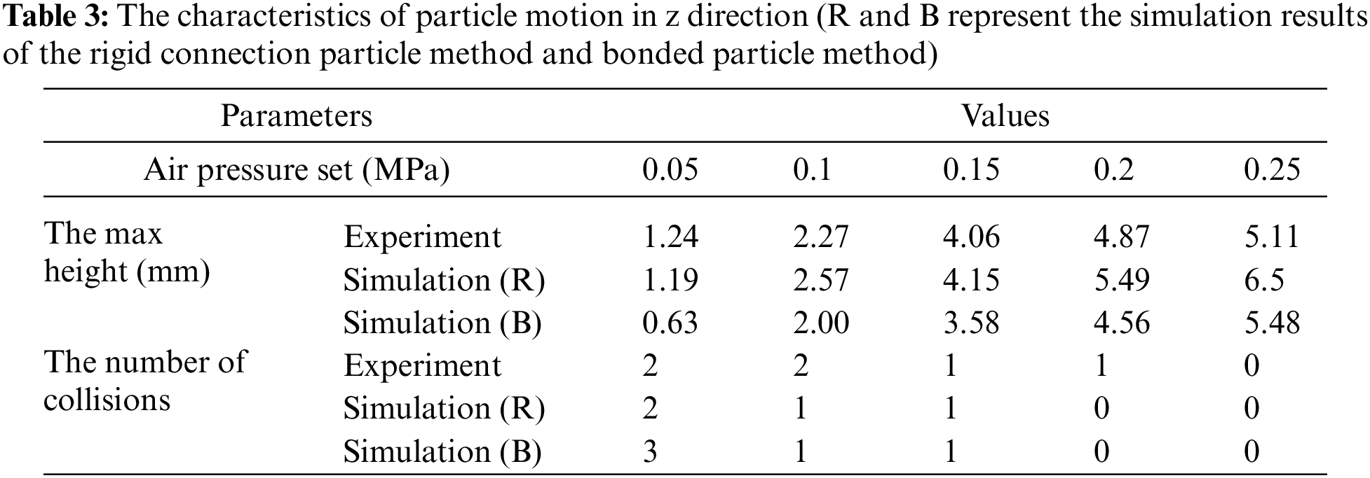
Therefore, for the several conditions involved in the standardized multi-particle experiment in this study, it can be considered that the proposed rigid connection particle method shows higher accuracy and greater applicability in describing large particle motion.
Simulations presented in this paper can be divided into three parts: in Sections 4.1 and 4.2, the rigid connection particle method is applied to simulations under DIN and SAE stone chip resistance standard test conditions. Simulated coating damage presented by wear model are compared with the experimental damage on the coating panel to prove the application value of this method. In Section 4.3, simulations are conducted to assess the performance of the proposed method to reproduce the difference of the coating damage under different impact velocity and test panel orientation conditions.
4.1 Multi-particle Simulation—DIN Standard
This simulation is established according to the DIN55996-1 standard experiment. Its schematic diagram and some relevant parameters are shown in Fig. 10. According to the experimental conditions, a circular pipe with a diameter of 30 mm is used as the acceleration pipe. 500 g chilled cast iron particles with edges and corners are uniformly injected into the pipeline within 10 s. The test panel with the size of 100 × 200 mm is obliquely placed at an angle of 54° to the horizontal plane and serves as a no-slip fixed wall. There are meshes on the coating panel used for region partition in the wear computation.

Figure 10: Schematic diagram of the simulation based on DIN standard experiment
In the experiment, flow conditions at the three-way pipe which connects the nozzle, the accelerating pipe, and the feeding tube are complicated. For the purpose of minimizing the computational cost, the model is simplified. The horizontal particle velocity at the inlet of accelerating pipe is measured through experiment, and it is set to be the initial velocity of particles once they generate in simulation. It can be concluded from experiments that the horizontal initial velocity is approximately proportional to the nozzle flow velocity, and negatively related to the equivalent diameter and density of the particles. It can be simply estimated by an empirical formula:
where
Simulation is then performed by using the simplified model, with the inlet of accelerating pipe being velocity-inlet, outlet of the protection box being pressure-outlet, and the wall being no slip boundary condition. A one-third sphere-shaped composite particle made up of 809 component spheres is used to approximately represent the chilled cast iron particle in experiment, and its shape is shown in Fig. 11. For the initial velocity of particle, the horizontal component is determined by Eq. (11), the vertical component is determined by the particle falling height and restitution coefficient. Furthermore, the air pressure is set to 0.1 MPa, and other parameters of DIN standard simulation is set to be the same with the single particle motion simulation in Section 3. The simulation time is set to be 1 s, for it is enough to show the distribution of particle impact.

Figure 11: The shape of particles used in DIN test and simulation (a) Chilled iron cast particle (b) Composite particle used in DIN simulation
The evaluation of the simulation results will be carried out from two aspects: particle impact velocity and particle impact damage distribution. For the assess of particle impact velocity, 30 particles in a continuous period are selected from experiment and simulation respectively, whose impact velocities as well as impact angles are compared in Fig. 12 and Table 4. The each scatter on Fig. 12 represents a certain particle impact in the experiment or in the simulation, with its coordinates indicating the impact velocity and impact angle of this particle impact. It is worth mentioning that the y direction component of impact velocity is often less than 1/25 of the x direction component, and is thus ignored in the calculation of impact angle. Generally, with respect to the average value, impact velocity and impact angle of the simulation agree well with that in experiment. Nevertheless, because the particle injection velocity is used as a replacement of the initial acceleration effect at the three-way pipe, the particle movement in simulation appears to be more regular and uniform, resulting in a smaller standard deviation and a narrower range of entrance angle, i.e., the direction of particle velocity at the outlet of accelerating pipe, as shown in Fig. 13. Also, the simulated impact velocity has a smaller span than that in experiment.

Figure 12: Comparison of simulated particle impact velocity and impact angle with DIN experimental results (Definition of the parameter α and v described in the right)


Figure 13: The difference in the range of entrance angle between DIN simulation and experiment (black solid line for experiment and red for simulation)
In terms of impact damage distribution, the picture of the coating panel after DIN standard test and the simulated coating damage presented by wear model are displayed in Fig. 14. The coating panel is evenly divided into five parts from top to bottom for the convenience of comparison and analysis. Impact damage distribution is defined as the proportion of impact damage on each part to the total impact damage, which is displayed in Fig. 15. As can be obtained from the experimental test panel, due to the projectiles’ numerousness as well as their sharp edges and corners, almost the entire panel is subjected to minor scratches and small area damage. Although the impact damage on the simulated test panel is less than that on the experimental one limited by the simulation time, the impact damage distribution can be clearly obtained. As shown in Fig. 15, the distribution in simulation is in consistence with experimental results, except that the overall impact position in simulation is lower than the experimental results due to the difference in entrance angle aforementioned. In addition, the simulation and experimental outcomes are in good agreement in showing that the impact on the middle part of the coating causes severer wear.

Figure 14: Damaged DIN coating panel of experiment (left) and simulation (right)

Figure 15: The impact damage distribution over different parts of DIN coating panel
4.2 Multi-Particle Simulation—SAE Standard
The simulation established according to the SAE J400-2002 standard experiment is shown in Fig. 16. According to the experimental conditions, a circular pipe with a diameter of 52 mm is used as the acceleration pipe, and 1pt pebbles are uniformly injected into the pipeline within 7 s. The coating panel with a size of 100 × 300 mm is placed vertically to the airflow direction and serves as a no-slip fixed wall. Meshes are divided on the coating panel used for region partition in the wear computation. The simulation is simplified based on the same principle in Section 4.1. Likewise, the gas inlet of the accelerating pipe is set as fixed value velocity inlet. The inlet velocity is set to be 31.1 m/s as is obtained from the flowmeter under the condition of 0.48 MPa air pressure setting. The outlet in the protection box is treated as fixed value pressure outlet with the value being 0. For brevity, other parameters are listed in Table 5.
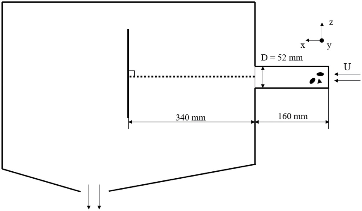
Figure 16: Schematic diagram of the simulation based on SAE standard experiment

By sorting and categorizing the pebbles used in the experiment, two ellipsoidal composite particles of different sizes, two rounded quadrangular pyramid composite particles of different sizes, i.e., a total of four kinds of composite particles are used to approximate the shape of the pebbles during the experiment. The shapes of the composite particles as well as the pebbles are shown in Fig. 17. The simulation time is set to be 2 s, for it is adequate to obtain the pattern of particle impact.

Figure 17: The shape of particles used in SAE test and simulation (a) instances of pebble particles (b) composite particle used in SAE simulation
In the experiment and simulation respectively, 30 particles are selected in succession with their trajectories recorded. The results are compared through a scatter diagram with the particle impact velocity v being the x coordinate and the impact angle α being the y coordinate, as shown in Fig. 18. The corresponding data is also analyzed in Table 6. Similar to Section 4.1, the y direction component of impact velocity is ignored. With respect to impact velocity, the simulated average particle velocity is in good agreement with that in the experiment. However, compared with the simulation results, the particle velocity in the experiment has a larger span. Apart from the influence of the injection velocity, the simplification of particle shape and density may also play an important role. The simulation and experiment are in accord in terms of impact angle from the aspects of average value and the standard deviation. Generally, the number of particles with an impact angle greater than 90° is more than those with an impact angle less than 90°, under the influence of gravity. The comparison of entrance angle between simulation and experiment is displayed in Fig. 19. Because of the high particle velocity and the short accelerating pipe in SAE simulation, the uniformly set initial velocity has little effect on the z direction velocity component and entrance angle.

Figure 18: Comparison of simulated particle impact with SAE experimental results (The definition of the parameter α and v described in the figure)


Figure 19: The difference in the range of entrance angle between SAE simulation and experiment (black solid line for experiment and red for simulation)
The picture of the coating panel after test and the coating damage presented by wear model in simulation is displayed in Fig. 20. To facilitate comparison and analysis, the coating panel is evenly divided into 6 parts from top to bottom. The impact damage distribution of experiment and simulation is displayed and compared in Fig. 21. The distribution is presented by the percentage of impact damage on each part to the total impact damage. It can be known that the particle impact is mostly concentrated in the lower middle position of the sample, with a small part of the damage located at the upper and lower parts of the coating. In addition, the simulated test panel shows similar pattern with the experimental one that the particle impacts in Part 4 and Part 5 cause larger damage area or more eroded mass.

Figure 20: Damaged SAE coating panel of experiment (left) and simulation (right)

Figure 21: The impact damage distribution over different parts of SAE coating panel
Also, compared with the DIN simulation in Section 4.1, the projectiles in the SAE simulation have greater mass and impact velocity, which means they have higher kinetic energy when impact. Therefore, the simulated eroded mass in the SAE standard simulation is much larger than that in the DIN standard simulation, and the deformation of the substrate of the SAE sample in test is much more pronounced than that of the DIN sample. However, the overall experimental damage area appears to be smaller than that on the DIN sample in test. Apart from the factor of projectile quantity, the sharp cast iron may have a greater ability to damage the surface of coating than rounded pebbles. This phenomenon also implies although the wear model can be served as a useful tool to predict impact damage distribution and relative damage area, it is not suitable for predicting damage area for experiments which use different coatings or different projectiles.
4.3 Multi-Particle Simulation–Parametric Studies
To further study the influence of impact velocity as well as impact angle on the impact damage, simulations with different test panel orientations and initial particle velocity are carried out. The parameter differences in each case are shown in Table 7. Four additional multi-particle simulations, M1 to M4, are conducted. Their results are compared with that of the case M0 which represents the original SAE simulation in Section 4.2. The wear state of panels after 40 particle impacts are compared and analyzed (The particle impact here also counts particles that hit the clamp or flying over the test panel). Fig. 22 shows the comparison of the eroded mass between the simulations of different initial velocity.


Figure 22: Simulated coating panel with different initial velocity (from left to right: M3, M0, M4)
Likewise, the sample is divided into six parts for analysis. The eroded mass and the impact damage distribution among different cases are showed in Fig. 23. It can be concluded from the figure that the eroded mass increases with the particle velocity, which is reasonable for that the impact wear is closely related to the kinetic energy of particles. It is also in accord with the conclusion of Nguyen et al. [6]. In terms of the impact position distribution, the overall impacted area appears to move down as the particle velocity goes up. This is possibly related to the decrease of the collisions between the particle and the accelerating pipe wall. More particles move out of the pipe without collision and impact the lower part of the test panel under the action of gravity. The upper and bottom parts of coating panel, which is defined as Part 1, Part 2 and Part 6, is rarely impacted by particles directly. Wear in these parts is basically caused by the secondary impact of the flying particle and thus varies a lot in different cases.

Figure 23: Coating damage under different initial velocity conditions (a) Eroded mass, (b) Impact damage distribution over 6 parts of coating panel
The comparison of the simulated eroded mass between the simulations of different panel orientations is presented in Fig. 24. Similarly, divided into 6 segments, the simulated coating panel is analyzed in Fig. 25. With the angle between the coating panel and the vertical plane increases, the particle impact is spreading to a larger part of the coating panel, which is due to the reduction of the projected area of the test panel on the YZ plane. Besides, as the impingement angle decreases from 90° to 54°, the eroded mass increases significantly, which is in good agreement with the conclusion made by Nguyen et al. [6,54].

Figure 24: Simulated coating panel with different panel orientation (from left to right: M0, M1, M2)

Figure 25: Coating damage under different panel orientation conditions (a) Eroded mass, (b) Impact damage distribution over 6 parts of coating panel
The above simulation results indicate that the simulation implemented with the rigid connection particle method and the Finnie wear model is able to reproduce the influence of particle velocity and impact angle on the impact damage of the test panel, further demonstrating the reliability of this method in predicting the impact damage on the test panel.
This work develops a CFD-DEM-wear model for stone chip resistance analysis of automotive coatings in a gravelometer test. Such complex physical phenomena normally involve fluid-particle interactions and impact wear of automotive coatings. In the developed method, the unresolved CFD-DEM method is employed to account for interactions between fluids and large particles, and a rigid connection particle method is proposed to facilitate the description of large particles using a number of non-overlapping rigidly connected spheres. The fluid-particle forces are initially calculated on each component sphere, and then converted to the resultant force and moment of larger particles based on the rigid connection. The proposed rigid connection particle method neatly avoids the local extreme of void fraction around particle centroid by making large particles physically porous, and the translation and rotation of non-spherical particles can be better represented. A Finnie wear model is used to calculate the impact damage of automotive coatings subjected to non-spherical particles.
Single- and multi-particle tests are performed to demonstrate the accuracy of the CFD-DEM coupling method in simulating spherical and non-spherical large particle movement in terms of motion trajectory. The developed CFD-DEM-wear coupling method is applied to evaluate stone chip resistance performance of automotive coatings in two standard gravelometer tests, i.e., DIN 55996-1 and SAE-J400-2002 tests. Numerical results are found in consistent with experimental data in terms of impact velocity and damage distribution, which validates the capacity of our developed method in stone chip resistance evaluation of automotive coatings. Finally, parametric studies are conducted to numerically investigate the effects of initial particle velocity and test panel orientation. Results show that when the initial velocity increases, the eroded mass increases as well, and the impacted area appears to be located in a lower position. In addition, from 90° to 54°, the increase of the angle between the test panel and the vertical plane will lead to the increase in the eroded mass and expansion of the area being impacted.
In the current study, the movement of particles near the high-pressure air nozzle is circumvented, so as to dramatically improve computational efficiency. Instead, an initial velocity obtained from the preliminary experiment is set for each particle to replace the acceleration effect. However, this numerical treatment will lead to mismatch of inlet boundary conditions for the stone chip resistance analysis, which contributes to the large differences between some experimental and numerical results. Our future works have scheduled to develop numerical methods to better describe the inlet boundary conditions for stone chip simulations.
Funding Statement: This work is supported by the National Key R&D Program of China (No. 2017YFE0117300), the Science and Technology Planning Project of Guangzhou (No. 201804020065), and the Innovation Group Project of Southern Marine Science and Engineering Guangdong Laboratory (Zhuhai) (No. 311021013).
Conflicts of Interest: The authors declare that they have no conflicts of interest to report regarding the present study.
Reference
1. Zhu, H. P., Zhou, Z. Y., Yang, R. Y., Yu, A. B. (2008). Discrete particle simulation of particulate systems: A review of major applications and findings. Chemical Engineering Science, 63(23), 5728–5770. DOI 10.1016/j.ces.2008.08.006. [Google Scholar] [CrossRef]
2. Kuang, S., Zhou, M., Yu, A. (2020). CFD-DEM modelling and simulation of pneumatic conveying: A review. Powder Technology, 365, 186–207. DOI 10.1016/j.powtec.2019.02.011. [Google Scholar] [CrossRef]
3. Ding, D., Liang, Y., Li, Y., Sun, J., Han, D.et al. (2019). Numerical study of trapped solid particles displacement from the elbow of an inclined oil pipeline. Computer Modeling in Engineering & Sciences, 121(1), 273–290. DOI 10.32604/cmes.2019.07228. [Google Scholar] [CrossRef]
4. Zhao, R. J., Zhao, Y. L., Zhang, D. S., Li, Y., Geng, L. L. (2021). Numerical investigation of the characteristics of erosion in a centrifugal pump for transporting dilute particle-laden flows. Journal of Marine Science and Engineering, 9(9), 961. DOI 10.3390/jmse9090961. [Google Scholar] [CrossRef]
5. Tang, C., Yang, Y. C., Liu, P. Z., Kim, Y. J. (2021). Prediction of abrasive and impact wear due to multi-shaped particles in a centrifugal pump via CFD-DEM coupling method. Energies, 14(9), 2391. DOI 10.3390/en14092391. [Google Scholar] [CrossRef]
6. Nguyen, V. B., Nguyen, Q. B., Lim, C. Y. H., Zhang, Y. W., Khoo, B. C. (2015). Effect of air-borne particle–particle interaction on materials erosion. Wear, 322–323, 17–31. DOI 10.1016/j.wear.2014.10.014. [Google Scholar] [CrossRef]
7. Zhong, W., Yu, A., Liu, X., Tong, Z., Zhang, H. (2016). DEM/CFD-DEM modelling of non-spherical particulate systems: Theoretical developments and applications. Powder Technology, 302, 108–152. DOI 10.1016/j.powtec.2016.07.010. [Google Scholar] [CrossRef]
8. Loth, E. (2008). Drag of non-spherical solid particles of regular and irregular shape. Powder Technology, 182(3), 342–353. DOI 10.1016/j.powtec.2007.06.001. [Google Scholar] [CrossRef]
9. Mandø, M., Rosendahl, L. (2010). On the motion of non-spherical particles at high reynolds number. Powder Technology, 202(1–3), 1–13. DOI 10.1016/j.powtec.2010.05.001. [Google Scholar] [CrossRef]
10. Mandø, M., Yin, C., Sørensen, H., Rosendahl, L. (2007). On the modelling of motion of non-spherical particles in two-phase flow. Proceedings of the 6th International Conference on Multiphase Flow, pp. 9–13. Leipzig, Germany. [Google Scholar]
11. Ganser, G. H. (1993). A rational approach to drag prediction of spherical and nonspherical particles. Powder Technology, 77(2), 143–152. DOI 10.1016/0032-5910(93)80051-B. [Google Scholar] [CrossRef]
12. Petit, H. A., Irassar, E. F., Barbosa, M. R. (2018). Evaluation of the performance of the cross-flow air classifier in manufactured sand processing via CFD–DEM simulations. Computational Particle Mechanics, 5(1), 87–102. DOI 10.1007/s40571-017-0155-6. [Google Scholar] [CrossRef]
13. Krumbein, W. C., (1941). Measurement and geological significance of shape and roundness of sedimentary particles. Journal of Sedimentary Research, 11(2), 64–72. DOI 10.1306/D42690F3-2B26-11D7-8648000102C1865D. [Google Scholar] [CrossRef]
14. Tran-Cong, S., Gay, M., Michaelides, E. E. (2004). Drag coefficients of irregularly shaped particles. Powder Technology, 139(1), 21–32. DOI 10.1016/j.powtec.2003.10.002. [Google Scholar] [CrossRef]
15. Wang, Y., Zhou, L., Yang, Q. (2019). Hydro-mechanical analysis of calcareous sand with a new shape-dependent fluid-particle drag model integrated into CFD-DEM coupling program. Powder Technology, 344, 108–120. DOI 10.1016/j.powtec.2018.12.008. [Google Scholar] [CrossRef]
16. Song, X., Xu, Z., Li, G., Pang, Z., Zhu, Z. (2017). A new model for predicting drag coefficient and settling velocity of spherical and non-spherical particle in newtonian fluid. Powder Technology, 321, 242–250. DOI 10.1016/j.powtec.2017.08.017. [Google Scholar] [CrossRef]
17. Lu, G., Third, J. R., Müller, C. R. (2015). Discrete element models for non-spherical particle systems: From theoretical developments to applications. Chemical Engineering Science, 127, 425–465. DOI 10.1016/j.ces.2014.11.050. [Google Scholar] [CrossRef]
18. Madhav, G. V., Chhabra, R. P. (1995). Drag on non-spherical particles in viscous fluids. International Journal of Mineral Processing, 43(1–2), 15–29. DOI 10.1016/0301-7516(94)00038-2. [Google Scholar] [CrossRef]
19. You, Y., Zhao, Y. (2018). Discrete element modelling of ellipsoidal particles using super-ellipsoids and multi-spheres: A comparative study. Powder Technology, 331, 179–191. DOI 10.1016/j.powtec.2018.03.017. [Google Scholar] [CrossRef]
20. Podlozhnyuk, A., Pirker, S., Kloss, C. (2017). Efficient implementation of superquadric particles in discrete element method within an open-source framework. Computational Particle Mechanics, 4(1), 101–118. DOI 10.1007/s40571-016-0131-6. [Google Scholar] [CrossRef]
21. Kruggel-Emden, H., Rickelt, S., Wirtz, S., Scherer, V. (2008). A study on the validity of the multi-sphere discrete element method. Powder Technology, 188(2), 153–165. DOI 10.1016/j.powtec.2008.04.037. [Google Scholar] [CrossRef]
22. Sun, R., Xiao, H., Sun, H. (2017). Realistic representation of grain shapes in CFD–DEM simulations of sediment transport with a bonded-sphere approach. Advances in Water Resources, 107, 421–438. DOI 10.1016/j.advwatres.2017.04.015. [Google Scholar] [CrossRef]
23. Li, Z., Zhang, P., Sun, Y., Zheng, C., Xu, L. (2021). Discrete particle simulation of Gas-solid flow in Air-blowing seed metering device. Computer Modeling in Engineering & Sciences, 127(3), 1119–1132. DOI 10.32604/cmes.2021.016019. [Google Scholar] [CrossRef]
24. Ren, B., Zhong, W., Chen, Y., Chen, X., Jin, B. et al. (2012). CFD-DEM simulation of spouting of corn-shaped particles. Particuology, 10(5), 562–572. DOI 10.1016/j.partic.2012.03.011. [Google Scholar] [CrossRef]
25. Jensen, A. L., Sørensen, H., Rosendahl, L., Adamsen, P., Lykholt-Ustrup, F. (2016). Investigation of drag force on fibres of bonded spherical elements using a coupled CFD-DEM approach. 9th International Conference on Multiphase Flow, Firenze, Italy. [Google Scholar]
26. Guo, Y., Wassgren, C., Ketterhagen, W., Hancock, B., James, B. et al. (2012). A numerical study of granular shear flows of rod-like particles using the discrete element method. Journal of Fluid Mechanics, 713, 1–26. DOI 10.1017/jfm.2012.423. [Google Scholar] [CrossRef]
27. Anderson, T. B., Jackson, R. (1967). Fluid mechanical description of fluidized beds. Equations of motion. Industrial & Engineering Chemistry Fundamentals, 6(4), 527–539. DOI 10.1021/i160024a007. [Google Scholar] [CrossRef]
28. Peng, Z., Doroodchi, E., Luo, C., Moghtaderi, B. (2014). Influence of void fraction calculation on fidelity of CFD-DEM simulation of gas-solid bubbling fluidized beds. AIChE Journal, 60(6), 2000–2018. DOI 10.1002/aic.14421. [Google Scholar] [CrossRef]
29. Wang, Z., Liu, M. (2020). Semi-resolved CFD–DEM for thermal particulate flows with applications to fluidized beds. International Journal of Heat and Mass Transfer, 159, 120150. DOI 10.1016/j.ijheatmasstransfer.2020.120150. [Google Scholar] [CrossRef]
30. Hager, A. (2014). CFD-DEM on multiple scales--An extensive investigation of particle-fluid interactions (Ph.D. Thesis). Johannes Kepler University Linz, Linz. [Google Scholar]
31. Cheng, K., Wang, Y., Yang, Q. (2018). A Semi-resolved CFD-DEM model for seepage-induced fine particle migration in gap-graded soils. Computers and Geotechnics, 100, 30–51. DOI 10.1016/j.compgeo.2018.04.004. [Google Scholar] [CrossRef]
32. Hager, A., Kloss, C., Pirker, S., Goniva, C. (2012). Parallel open source CFD-DEM for resolved particle-fluid interaction. Proceedings of 9th International Conference on Computational Fluid Dynamics in Minerals and Process Industries, Melbourne, Australia. [Google Scholar]
33. Huang, W. X., Tian, F. B. (2019). Recent trends and progress in the immersed boundary method. Proceedings of the Institution of Mechanical Engineers, Part C: Journal of Mechanical Engineering Science, 233(23–24), 7617–7636. DOI 10.1177/0954406219842606. [Google Scholar] [CrossRef]
34. Hoomans, B. P. B., Kuipers, J. A. M., Briels, W. J., van Swaaij, W. P. M. (1996). Discrete particle simulation of bubble and slug formation in a two-dimensional gas-fluidised bed: A hard-sphere approach. Chemical Engineering Science, 51(1), 99–118. DOI 10.1016/0009-2509(95)00271-5. [Google Scholar] [CrossRef]
35. Link, J. M., Cuypers, L. A., Deen, N. G., Kuipers, J. A. M. (2005). Flow regimes in a spout–fluid bed: A combined experimental and simulation study. Chemical Engineering Science, 60(13), 3425–3442. DOI 10.1016/j.ces.2005.01.027. [Google Scholar] [CrossRef]
36. Jing, L., Kwok, C. Y., Leung, Y. F., Sobral, Y. D. (2016). Extended CFD-DEM for free-surface flow with multi-size granules: CFD-DEM for free-surface flow. International Journal for Numerical and Analytical Methods in Geomechanics, 40(1), 62–79. DOI 10.1002/nag.2387. [Google Scholar] [CrossRef]
37. Xiao, H., Sun, J. (2011). Algorithms in a robust hybrid CFD-DEM solver for particle-laden flows. Communications in Computational Physics, 9(2), 297–323. DOI 10.4208/cicp.260509.230210a. [Google Scholar] [CrossRef]
38. Yang, Q., Cheng, K., Wang, Y., Ahmad, M. (2019). Improvement of semi-resolved CFD-DEM model for seepage-induced fine-particle migration: Eliminate limitation on mesh refinement. Computers and Geotechnics, 110, 1–18. DOI 10.1016/j.compgeo.2019.02.002. [Google Scholar] [CrossRef]
39. Zhu, G., Li, H., Wang, Z., Zhang, T., Liu, M. (2021). Semi-resolved CFD-DEM modeling of gas-particle two-phase flow in the micro-abrasive air jet machining. Powder Technology, 381, 585–600. DOI 10.1016/j.powtec.2020.12.042. [Google Scholar] [CrossRef]
40. Xiong, S., Chen, S., Zang, M., Makoto, T. (2021). Development of an unresolved CFD-DEM method for interaction simulations between large particles and fluids. International Journal of Computational Methods, 18(10), 2150047. DOI 10.1142/S021987622150047X. [Google Scholar] [CrossRef]
41. Finnie, I. (1960). Erosion of surfaces by solid particles. Wear, 3(2), 87–103. DOI 10.1016/0043-1648(60)90055-7. [Google Scholar] [CrossRef]
42. Tsuji, Y., Kawaguchi, T., Tanaka, T. (1993). Discrete particle simulation of two-dimensional fluidized bed. Powder Technology, 77(1), 79–87. DOI 10.1016/0032-5910(93)85010-7. [Google Scholar] [CrossRef]
43. Cundall, P. A., Strack, O. D. L. (1979). A discrete numerical model for granular assemblies. Géotechnique, 29(1), 47–65. DOI 10.1680/geot.1979.29.1.47. [Google Scholar] [CrossRef]
44. Ball, R. C., Melrose, J. R. (1997). A simulation technique for many spheres in quasi-static motion under frame-invariant pair drag and brownian forces. Physica A: Statistical Mechanics and its Applications, 247(1), 444–472. DOI 10.1016/S0378-4371(97)00412-3. [Google Scholar] [CrossRef]
Hertz, H. (1881). On the contact of elastic solids. Journal of für die Reine und Angewandte Mathematik, 92, 156–171. DOI 10.1515/9783112342404-004. [Google Scholar] [CrossRef]
46. Mindlin, R. D. (1949). Compliance of elastic bodies in contact. Journal of Applied Mechanics, 16, 259–268. DOI 10.1115/1.4009973. [Google Scholar] [CrossRef]
47. di Renzo, A., di Maio, F. P. (2005). An improved integral non-linear model for the contact of particles in distinct element simulations. Chemical Engineering Science, 60(5), 1303–1312. DOI 10.1016/j.ces.2004.10.004. [Google Scholar] [CrossRef]
48. Zhu, H. P., Zhou, Z. Y., Yang, R. Y., Yu, A. B. (2007). Discrete particle simulation of particulate systems: Theoretical developments. Chemical Engineering Science, 62(13), 3378–3396. DOI 10.1016/j.ces.2006.12.089. [Google Scholar] [CrossRef]
49. di Felice, R. (1994). The voidage function for fluid-particle interaction systems. International Journal of Multiphase Flow, 20(1), 153–159. DOI 10.1016/0301-9322(94)90011-6. [Google Scholar] [CrossRef]
50. Kodam, M., Bharadwaj, R., Curtis, J., Hancock, B., Wassgren, C. (2009). Force model considerations for glued-sphere discrete element method simulations. Chemical Engineering Science, 64(15), 3466–3475. DOI 10.1016/j.ces.2009.04.025. [Google Scholar] [CrossRef]
51. Kloss, C., Goniva, C., Hager, A., Amberger, S., Pirker, S. (2012). Models, algorithms and validation for opensource DEM and CFD-DEM. Progress in Computational Fluid Dynamics, an International Journal, 12(2/3), 140. DOI 10.1504/PCFD.2012.0474574. [Google Scholar] [CrossRef]
52. Jasak, H., Jemcov, A., Tukovic, Z. (2007). OpenFOAM: A C++ library for complex physics simulations. International Workshop on Coupled Methods in Numerical Dynamics, vol. 1000, pp. 1–20. IUC Dubrovnik, Croatia. [Google Scholar]
53. Kloss, C., Goniva, C. (2011). LIGGGHTS–Open source discrete element simulations of granular materials based on lammps. Supplemental Proceedings: Materials Fabrication, Properties, Characterization, and Modeling, 2, 781–788. DOI 10.1002/9781118062142.ch94. [Google Scholar] [CrossRef]
54. Eraky, M. T., Elmelegy, T., Shazly, M., Eltayeb, N. S. M. (2018). A combined CFD-solid finite element model to study the mechanics of sand erosion damage in coated glass fiber reinforced polymer. ASME International Mechanical Engineering Congress and Exposition, V009T12A052. DOI 10.1115/IMECE2018-87966. [Google Scholar] [CrossRef]
 | This work is licensed under a Creative Commons Attribution 4.0 International License, which permits unrestricted use, distribution, and reproduction in any medium, provided the original work is properly cited. |