Computer Modeling in Engineering & Sciences

---

DOI: 10.32604/cmes.2022.020335

ARTICLE

Hysteresis of Dam Slope Safety Factor under Water Level Fluctuations Based on the LEM Coupled with FEM Method

Guodong Liu1,2,*, Zhijun Zhou1, Shiqiang Xu1 and Wenjing Mi2

1School of Highway, Chang’an University, Xi’an, 710046, China
2College of Urban, Rural Planning and Architectural Engineering, Shangluo University, Shangluo, 726000, China
*Corresponding Author: Guodong Liu. Email: 2017021006@chd.edu.cn
Received: 17 November 2021; Accepted: 22 February 2022

1  Introduction

Practice has revealed that water level fluctuations have significant effects on the dam slope safety factor (FS) and can result in huge casualties to the people in the vicinity. A considerable proportion of dam slope failures around the world are triggered by water storage in reservoirs. Based on previous studies, 49% of the slope sliding events near Roosevel Lake between 1941 and 1942 were triggered by water storage and 30% were triggered by water release [1]. Similarly, the slope sliding events on the left bank of the Vaiont reservoir between 1960 and 1963 were triggered by water storage [2]; 60% of Japan’s reservoir slope failure events were triggered by water release and 40% were triggered by water storage [3]. Other examples include the Pilarcitos Dam failure south of San Francisco, California, USA, the Walter Boudin Dam failure in Alabama in the United States, and many river bank slope failures along the Rio Montaro in Peru [4]. In an effort to protect the lives and property of people living near dams from dam failure, this issue has received increasing attention from researchers [5–7].

Generally, the FS of a dam slope is influenced by both the hydrostatic pressure and the pore water pressure (matrix suction if it is negative) [8,9]. The hydrostatic pressure acting on the surface of the slope contributes to the stability of the slope, which is favorable to dam safety [10,11]. Consequently, when the water level decreases, the FS of the dam slope must decrease if the influence of the decrease in the free surface is neglected in this process. However, the free surface also decreases along the sides, which complicates the problem more [12,13]. Lane et al. [14,15] found that the FS initially decreased and then increased during the drawdown process, which was manifested as the effect of the tradeoff between the increase in the soil weight and the shear resistance. Thus, a minimum FS value for water level fluctuations. Gao et al. [16] studied the effect of water drawdown on the three-dimensional slope safety factor and found that the variation of FS of the dam slope was non-monotonic and was due to the tradeoff between the hydrostatic pressure and the pore water pressure.

Furthermore, fluctuations in the water level can induce a change in the angle of the matrix suction friction and the unit weight, subsequently inducing a change in the slope safety factor. Current slope stability analysis under seepage adopts the Fredlund and Morgenstern’s dual variables model [17], which assumes that the soil’s strength is affected by both the net normal stress and the suction. To incorporate the matrix suction into the analysis, the seepage calculation should involve the soil–water characteristic curve (SWCC). Nuria et al. [18] demonstrated that the SWCC has a significant influence on the seepage. When the air entry value increased, the free surface decreased. However, the effect of the SWCC hysteresis on the slope safety factor is still unclear.

In recent years, more studies have concentrated on dam slope stability during water level variations and some have considered the SWCC. Wang et al. [19] studied the stability of an earth dam using multivariate adaptive regression splines with respect to the water level fluctuations, and they concluded that the earth dam slope failure probability is significantly influenced by the water level fluctuation rate and the soil friction angle. Sun et al. [20] investigated earth dam stability during water level drawdown and rainfall, and they found that the earth dam slope stability is considerably influenced by the permeability coefficient, porosity, and saturation when the water level fluctuations and rainfall are considered in a combined manner. These studies can be broadly classified into three groups: (1) numerical simulations [21–24]; (2) field investigation and monitoring data analysis [25–29]; and (3) model tests [30–34]. As was demonstrated by Duncan [35], numerical simulations have the advantages of being economical, convenience, and time-saving, and they can be developed and adopted in various aspects [36–39].

Although many studies have been conducted on dam stability under water level fluctuations, the results are not sufficient to direct engineering projects because previous studies did not take into account the hysteresis of the SWCC in addition to the FS. As would be expected, the change in the free surface with water level fluctuations has a duration, which in turn causes a lag in the FS of the dam slope. Thus, the variation curve of the slope safety factor with water level fluctuations should contain a hysteresis loop. The study of the FS hysteresis loop under SWCC hysteresis is of great importance to engineering projects.

Based on an actual earth dam in China, in this study, the finite element software Geo-studio was used to analyze the FS of the dam slope during water level fluctuations. First, the soil parameters were obtained through geotechnical experiments, including direct shear tests and permeability tests. Second, a numerical model was constructed using the Geo-studio software, within which the seep/w module was used to calculate the seepage field and the slope/w module was used to calculate the FS of the dam slope. Additionally, the SWCC hysteresis and the water level fluctuation rate were taken into account in the calculation to investigate their influences on the FS of the dam slope. Finally, the FS data for the dam slope under water level drawup were used to construct prediction equations for the FS under water level drawdown, which facilitate the earth dam construction and operation for dam structures identical to that analyzed in this study.

2  Study Area

Hanyu reservoir is located on the Hanyu River in Hu County, Shaanxi province (Fig. 1). It was constructed in 1970 from homogeneous cohesive soil. Through field investigations, the upper layer of the river bed was found to be composed of sandy gravel underlain by red clay. Owing to the high permeability of the sandy gravel layer beneath the dam body, some anti-permeating measures were needed.

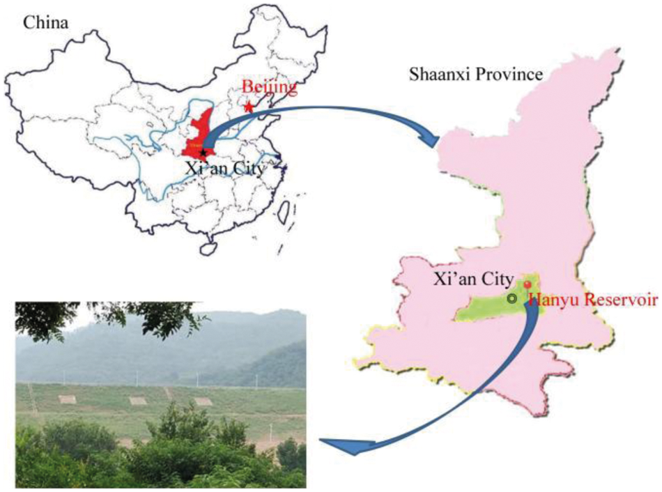
Figure 1: Map showing the location of the study area

The catchment area of the dam is about 11.7 km2, with an annual precipitation of approximately 591.1 mm. The precipitation is mainly concentrated in summer, so the reservoir water level is usually at a normal elevation of 568.90 m during the summer; while during the dry season it can fall to the sedimentation elevation of 559.40 m. It can be reasonably concluded that the reservoir’s water level fluctuates between 568.90 m and 559.40 m with the seasons.

As Fig. 2 shows, the height of the dam is 34 m, and the widths of the crest and base are 8 m and 198 m, respectively. It was constructed with four different slope ratios along the upstream and downstream faces to meet the stability requirements.

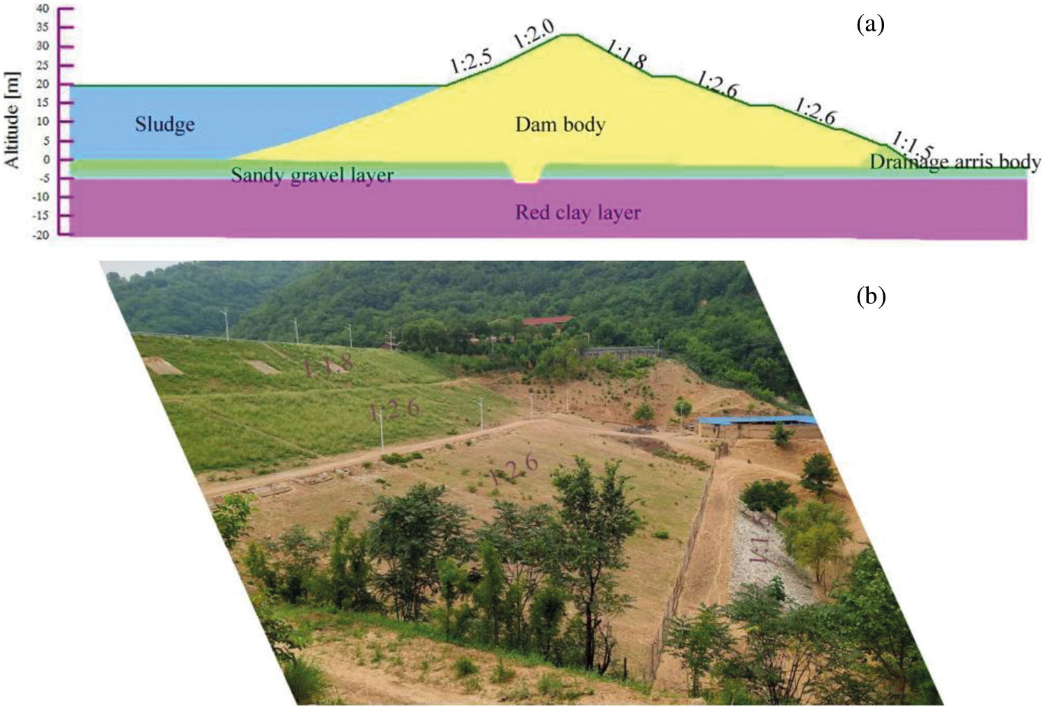
Figure 2: Project configuration: (a) typical cross section and (b) field photo

3  Analysis Scheme and Soil Properties

3.1 Seepage Analysis Theory

In the case of reservoir water level fluctuations, calculating the seepage of the dam is a transient seepage problem, in which the output variables are related to time [4]. Sufficient calculation theories have been developed to solve this problem, of which the finite element method (FEM) in the Geo-studio software is more satisfactory and thus was used in this study. In this calculation process, the permeability of the soils must be determined first because it varies with the saturation of the soils.

Genuchten et al. [40] developed an equation to predict the soil permeability that incorporates the saturated and unsaturated conditions using the SWCC. It can satisfactorily depict the relative hydraulic conductivity of a cohesive soil which is the ratio of the soil permeability to the saturated permeabiltiy and is expressed as Eq. (1):

Kr(p)=[1−(αp)(n−1)(1+(αp)n)−m]2[1+(αp)n]m2,(1)

where Kr(p) is the relative hydraulic conductivity; p is the pressure head in the soil; and α, m, and n are the parameters from the SWCC, which are related to the air entry value, the slope of the main section of the SWCC, and the residual water content of the soil, respectively. These parameters can be obtained from special experiments, which will be discussed later. It should be noted that the parameter n can be determined using Eq. (2):

n=1(1−m).(2)

And the SWCC which depicts the relation between the volumetric water content and the pressure head is expressed as:

θ−θrθs−θr=[11+(αp)n]m,(3)

where θ is the volumetric water content in the soil; θs, θr are the saturated and residual volumetric water contents, respectively; the other symbols are the same as in Eq. (1). It should be noted that from the volumetric water content θ the saturation degree Sr can be determined, as follows:

Sr=1+eeθ,(4)

where e denotes the void ratio of the soil. Thus, through Eqs. (3) and (4) the saturation degree Sr and the pressure head p can be related.

Then, by incorporating the SWCC and considering Darcy’s law, the following governing Eq. (5) can be derived:

∂∂x(kx∂h∂x)+∂∂z(kz∂h∂z)+S=∂θ∂t,(5)

where kx and ky are the horizontal permeability and the vertical permeability, respectively; S is the water storage or release, for which a positive value indicates storage and a negative value indicates release; h is the total water head; and θ is the volumetric water content needed in the SWCC.

From the SWCC we can derive Eq. (6):

∂θ∂t=m2w∂p∂t=m2wρwg∂(h−z)∂t=m2wρwg∂h∂t,(6)

where m2w is the slope of the SWCC at a certain point; ρw is the density of water; g is the acceleration of gravit. Letting λ=m2wρwg, Eq. (5) transforms into Eq. (7):

∂∂x(kx∂h∂x)+∂∂z(kz∂h∂z)+S=λ∂h∂t,(7)

where λ is the water storage coefficient. For two dimensional problems, the following conditions depicted by Eq. (8) need to be met:

h|t=0=H0(x,z)(x,z)∈Dh|Γ1=φ(x,z)(x,z)∈Γ1,t>012[kx∂h∂xcos⁡(n^x)+kz∂h∂zcos⁡(n^z)]|Γ2=qt>0.(8)

Here, H0(x, y) is the initial water head; φ(x,z) is the water head function on the first category of boundary Γ1; q is the single width feeding quantity on the second category of boundary; (n^x), (n^z) denote the angles between the X-axis, the Z-axis and the outer normal line of Γ2.

From the above, the following functional (Eq. (9)) can be established:

I(h)=∬D[12kx(∂h∂x)2+12kz(∂h∂z)2+Sh+λ∂h∂th]dxdz+∫ΓqhdΓ.(9)

The solving of the seepage problem under water fluctuations is equivalent to finding the minimum value of this functional. For a given element, this functional can be decomposed as Eq. (10):

Ie(h)=I1e+I2e+I3e+I4e,(10)

which is detailed as Eq. (11):

I1e=∬De12[kx(∂h∂x)2+kz(∂h∂z)2]dxdzI2e=∬DeShdxdzI3e=∬Deλh∂h∂tdxdzI4e=∫ΓqhdΓ.(11)

The water heads in an element can be obtained by interpolating the water heads of all the element nodes, which is expressed as the follows:

h=∑k=1nNkhk,(12)

where h is the water head in the element; hk is the water head of each element node; Nk is the interpolation function.

For each nodal head h1, h2, h3, …, hn, the partial derivative of I1e can be obtained as:

∂I1e∂hi=∬De12[kx∂∂hi(∂h∂x)2+kz∂∂hi(∂h∂z)2]dxdz.(13)

Substituting Eq. (12) into Eq. (13), we can obtain Eq. (14):

∂I1e∂hi=∑k=1mhk∬De[kx∂Nk∂x∂Nj∂x+kz∂Nk∂z∂Nj∂z]dxdz.(14)

Letting Kij=∬De[kx∂Ni∂x∂Nj∂x+kz∂Ni∂z∂Nj∂z]dxdz, we can obtain Eq. (15):

{∂I1e∂h}=[K11K12⋯K1nK21K22⋯K2n⋮⋮⋮⋮Kn1Kn2⋯Knn](h1h2⋮hn)=[K]e{h}e.(15)

Similarly, for each nodal head h1, h2, h3, …, hn, deriving the partial derivative of I2e with Eq. (12) substituted into, we can get Eq. (16):

∂I2e∂hi=S∬De∂∂hi(∑k=1nNkhk)dxdz=S∬DeNidxdz.(16)

Letting Ei=S∬DeNidxdz, it then has Eq. (17):

{∂I2e∂h}={E}e.(17)

For each nodal head h1, h2, h3, …, hn, deriving the partial derivative of I3e with Eq. (12) substituted into, we can get Eq. (18):

∂I3e∂hi=∑k=1n∂hk∂tλ∬DeNkNidxdz.(18)

Letting Rij=λ∬DeNkNidxdz, it then has Eq. (19):

{∂I3e∂h}=[R]e{∂h∂t}e.(19)

For each nodal head h1, h2, h3, …, hn, deriving the partial derivative of I4e with Eq. (12) substituted into, we can get Eq. (20):

∂I4e∂hi=∑k=1nqk∫De∩Γ2NkNidΓ.(20)

Letting Dij=∫De∩Γ2NiNjdΓ, it then has Eq. (21):

{∂I4e∂h}=[D]e{q}e.(21)

Thus, for each element, it has Eq. (22):

{∂I∂h}e=[K]e{h}e+{E}e+⌊R⌋e{∂h∂t}e+[D]e{q}e.(22)

Assembling the partial derivatives of the functional of all the elements with respect to h, which was made to equal to 0, we get:

[K]{h}+[R]{dhdt}=−{E}−[D]{q}+{F}.(23)

Here, {E} reflects the water storage or release; −[D]{q}+{F} reflects all the boundary conditions. Thus, the right-hand side of Eq. (23) can be merged into {Q}. Then we can get:

[K]{h}+[R]{dhdt}={Q}.(24)

For saturated-unsaturated seepage problems, Eq. (24) can be illustratively depicted as Eq. (25):

[Ks]{h}−[Kus]{h}+[Rs]{dhdt}−[Rus]{dhdt}={Q},(25)

where [Ks] is the permeability coefficient matrix of the saturated elements, [Kus] is the permeability coefficient matrix of the unsaturated elements, [Rs] is the water storage matrix of the saturated elements, [Rus] is the water storage matrix of the unsaturated elements, {h} is the nodal head vectors, and {Q} is the vector of the prescribed nodal flow referring to the boundary conditions. By solving this equation for each node within the discretized calculation domain, the seepage field of the domain can be obtained.

It should be noted that, [K] and [R] in Eq. (24) can be obtained by numerical integration, and the solution algorithm of this equation adopted back difference method, as Eq. (26):

([K]+[R]Δt){h}t+Δt=[R]Δt{h}t+[Q].(26)

3.2 Slope Stability Analysis Theory

The traditional approach to analyzing slope stability is the limit equilibrium method (LEM), which considers the saturated soil strength. While many other methods have been developed, the LEM is still the most reliable and acceptable method in geotechnical studies. More importantly, the unsaturated soil strength has been adopted in the LEM, which has extended this method to unsaturated soils [41]. In this study, the influence of water level fluctuations on the dam slope stability was investigated using Geo-studio, which incorporates unsaturated soil theory.

When calculating the safety factors, Eq. (27) formulated by Fredlund et al. [17] was adopted.

τf=c′+(σn−μa)tgφ′+(μa−μw)tgφb,(27)

where c′ is the effective cohesion, φ′ is the effective frictional angle, φb is the angle of the suction friction, σn is the net normal stress, μa is the pore air pressure, and (ua–uw) is the matrix suction in the soil.

The Morgenstern–Price method [8] meets the equilibrium requirements of both the force and the moment, and therefore, it is considered to be the strictest LEM. From the equilibrium of moment, a safety factor can be derived as Eq. (28):

Fm=∑(c′βR+[N−uwβtan⁡ϕbtan⁡ϕ′−uaβ(1−tan⁡ϕbtan⁡ϕ′)])Rtan⁡ϕ′∑Wx−∑Nf+∑kWe+∑Dd+Aa,(28)

where R is the sliding circle radius or the moment arm, k is the earthquake acceleration coefficient, e is the vertical distance from the soil slice centroid to the moment center, d is the perpendicular distance from the external line load to the center of the moment, a is the perpendicular distance from the external water force to the center of the moment, β is the slice base width, N is the normal force on the bottom of the slice, uw is the pore water pressure, ua is the pore air pressure, W is the slice weight, x is the horizontal distance from the slice centerline to the moment center, f is the perpendicular distance from the normal force line on the slice bottom to the moment center, D is the external load, and A is the external water force. The meanings of the other symbols are the same as above.

Another safety factor can be derived from the force equilibrium as follows:

Ff=∑(c′βcos⁡α+[N−uwβtan⁡ϕbtan⁡ϕ′−uaβ(1−tan⁡ϕbtan⁡ϕ′)]tan⁡ϕ′cos⁡α)∑Nsin⁡α+α∑kW−∑Dcos⁡ω±∑A,(29)

where α is the angle between the tangent on the center of the bottom of the slice and the horizontal line. The meanings of other symbols are the same as in Eq. (28). The frictional force between the slices can be calculated using an inter-slice function, which is not presented due to space limitations. As was defined by Morgenstern, the safety factor obeying both Eqs. (28) and (29) is considered to be the real safety factor. To identify the critical sliding surface, the Siegel grid method developed by Siegel et al. [41] was adopted in this study, which is described in detail by Siegel et al. [41].

3.3 Analysis Scheme

The profile of the dam analyzed in this study is shown in Fig. 2, in which (a) is a typical section and (b) is a field photo of the dam. The four different slope ratios of the upstream slope were 1:2.0, 1:2.5, 1:3.0, and 1:3.5, while the four different slope ratios of the downstream slope were 1:1.8, 1:2.6, 1:2.6, and 1:1.5.

For convenience, the origin of the coordinates was set as the toe of the upstream slope. The highest water level was 28.9 m (the normal water level) and the lowest water level was 19.4 m (the sedimentation elevation). The water level rose from 19.4 m to 28.9 m, stayed at this level for 6 days, and then dropped to 19.4 m at a constant rate. The variations in the water level of the reservoir used in this study are intuitively shown in Fig. 3. There were five cases represented by five different water level fluctuation rates (1 m/d, 2 m/d, 3 m/d, 4 m/d, and 5 m/d) for water level drawup and drawdown. The five different water level fluctuation rates were considered using five different boundary conditions on the upstream slope surface A-A-A in the software. The downstream slope surface was set as the potential seepage boundary, and the other edges of the model were set as impervious boundaries.

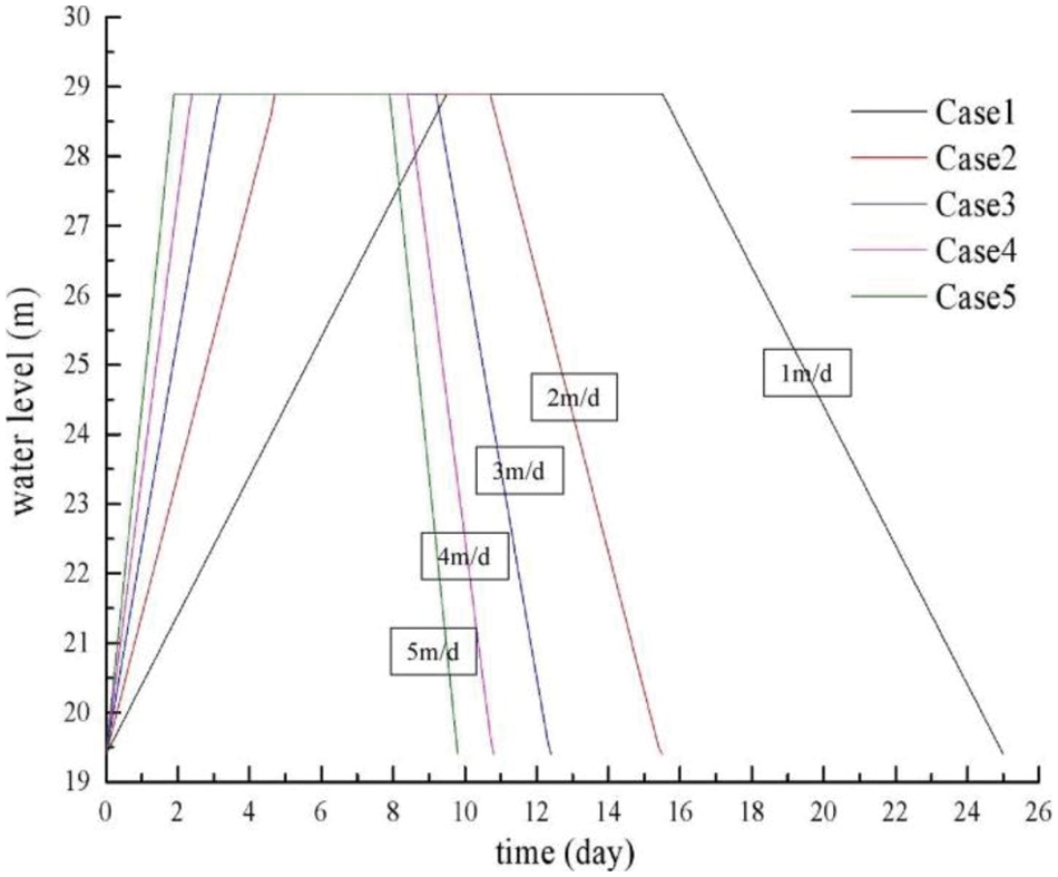
Figure 3: The varying reservoir water level of each case

The FEM model and the discrete grid of the dam are shown in Fig. 4, in which both three-node triangular elements and four-node quadrilateral elements were used to adapt to the complex shape of the dam model. A total of 3125 elements, including 2011 triangular elements and 1114 quadrilateral elements, were used in the model, which contained 2239 nodes.

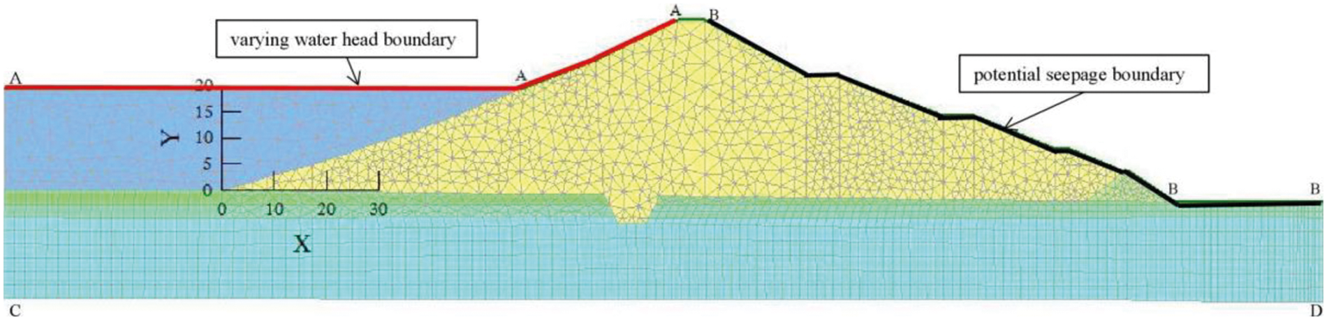
Figure 4: The FEM model and discrete grid of the dam. A-A-A is the variable water head boundary; B-B-B is the potential seepage boundary; and the other edges of the model are impervious boundaries

3.4 Material Parameters

There were six materials involved: the dam body material, the silt in front of the dam, the drainage arris body, the loam layer, the sandy gravel layer, and the red clay layer. In contrast to saturated seepage problems, in this study, unsaturated permeating problems, which refers to a varying permeability delineated by a permeability function, were incorporated. In this study, the permeability function estimated using the Van Genuchten theory [40], which depends on the SWCC and the saturated permeability coefficient, was used. As was demonstrated by Van Genuchten, the SWCC has different parameters under desorption and adsorption processes, thus inducing different unsaturated permeability coefficients. Since we were only concerned with the influence of the SWCC hysteresis formed under adsorption-desorption processes on the dam slope’s stability and the soil type of the dam body and its saturated permeability coefficients from indoor tests were nearly identical with those of Van Genuchten [40], the SWCC parameters for desorption and adsorption of Van Genuchten’s study were used. The values of the parameters are listed in Tables 1 and 2, and the meaning of each parameter was described by Dawson et al. [36]. It should be noted that only the adsorption SWCC parameters of the dam body are given here because the other materials were always below the free surface and were constantly saturated. The SWCC used is intuitively shown in Fig. 5, i.e., a hysteresis loop.

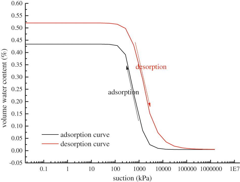
Figure 5: Hysteresis of the SWCC

The saturated permeability coefficients of all of the materials were determined through variable head permeability experiments, that is, the water head applied on the the specimen in the test was varied. First, the sample specimens were collected in the field using ring knives. Then, the samples were weighed using a balance to calculate the density of the specimens. Finally, the specimens were placed in the permeameter to determine the permeability coefficients (Kh) of the soils. The permeability experiment steps are shown in Fig. 6.

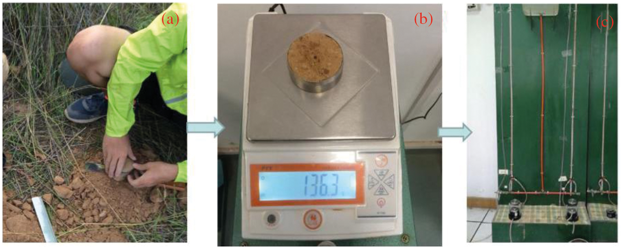
Figure 6: Permeability test process

The Mohr-Coulomb criterion, which has been extended to consider the influence of the matrix suction, was used to describe the shear strengths of the model materials due to its conciseness and wide acceptance. The shear strength parameter values essential in the slope stability analysis were determined through indoor direct shear experiments, and the density of each material was tested using the aforementioned ring knife experiment. The strength parameter values and the densities are presented in Table 3. To be more persuasive, Fig. 7 shows the direct shear test scenario.

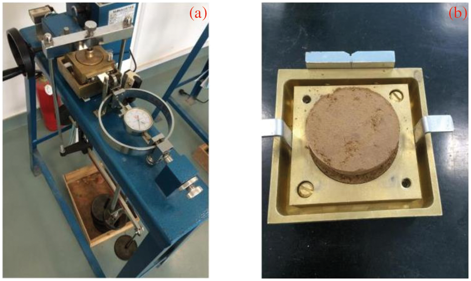
Figure 7: Direct shear experiment

4  Free Surface under Water Level Fluctuations

To detail the free surface variation subject to the water level fluctuations, the FEM model in Fig. 4 was employed with the varying water head applied on the upstream face (A-A-A). The seep/w tool was used to calculate the seepage under the water level fluctuations, in which the adsorption SWCC and the desorption SWCC were taken into account. Because we just concerned about the influences of the hysteresis of the SWCC on the free surface, only one water level fluctuation rate of 1 m/d was considered here. A vertical line (E–E) was drawn from the upstream slope shoulder, and a horizontal line with the elevation of 0 m was drawn as the base line. The definition of the free surface height was the distance between the intersection point of the base line and the vertical line and the intersection point of the free surface and the vertical line.

Fig. 8 presents the variation of the free surface under the water level fluctuation, with Fig. 8a referring to the situation of adsorption SWCC and Fig. 8b referring to the situation of desorption SWCC. Apparently, the free surface rose up with the rising of the reservoir water level, and vise vs. The variation of the free surface was more dramatic and swift near the upstream slope surface, and was negligible near the drainage arris body, which formed a horn shape area of free surface variation. It could be found that at the same reservoir water level the free surface height of the water level drawdown was greater that of the water level drawup. Thus, under the same reservoir water level, the free surfaces of water level drawup and drawdown formed a closed hysteresis loop, which was bigger and bigger as the water level variation time lasted. That could be mainly due to the water holding effect of the dam body soils. As the water level drawdown, the free surface could not decrease timely for the water holding effect of the dam body soils, thus causing the difference between the free surfaces of water level drawdown and drawup, which formed the hysteresis loop. The held water in the dam body accumulated more and more as the water level variation time lasted, which resulting in the larger and larger hysteresis loop.

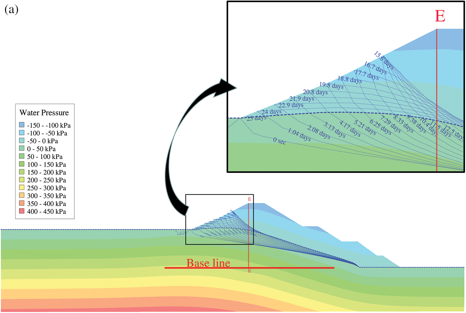
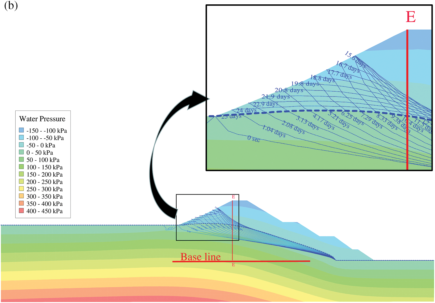
Figure 8: Free surface under water level fluctuations: (a) with the adsorption SWCC; (b) with the desorption SWCC

Comparing Figs. 8a and 8b, the variation rules of the free surface with the water level under both the adsorption SWCC and the desorption SWCC are identical. However, the free surface variation extent was different under the two situations, which can be more clearly seen in Fig. 9.

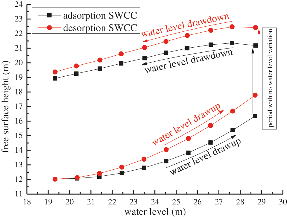
Figure 9: Free surface height during water level fluctuations

As can be seen in Fig. 9, the free surface height increased with the rising of the water level, and decreased with the declining of the water level. In the duration of the six days between the water level drawup and drawdwon, the free surface height continually increased. Comparably, the free surface increasing rate of the desorption SWCC during the water level drawup was greater than that of the adsorption SWCC, leading to the approximately 1 m larger free surface height of the desorption SWCC comparing with that of the adsorption SWCC at the end of the water level drawup. That could be due to the larger permeability coefficient at the unsaturated condition estimated from the adsorption SWCC, which vented the seepage water, thus lowering the free surface. The free surface height increments of the adsorption SWCC and the desorption SWCC are almost identical during the six days of no water level variation. That is, the difference of the free surface height between the adsorption SWCC and the desorption SWCC was still about 1 m at the beginning of the water level drawdown. However, as the water level drawdown, the difference between them gradually decreased, which could be due to the larger water holding capacity from the adsorption SWCC. Summarily, the free surface height of the desorption SWCC is larger than that of the adsorption SWCC, which is more evident with higher reservoir water levels. As the higher free surface is adverse to the dam safety, the desorption SWCC is suggested for the engineering practice.

5  FS of Upstream Dam Slope under Water Level Fluctuations

Broadly utilized in the geotechnical field, the safety factor is commonly accepted as the only recognized indicator for evaluating slope stability under various conditions, including under water level fluctuations. Earth filled dams under water level fluctuation exactly describes this problem, and their FS values also fluctuate wildly.

5.1 FS under Water Level Drawup–Drawdown Cycles

To investigate the dam slope stability under water level drawup–drawdown cycles, The calculated seepage field was input into the slope/w tool to calculate the slope stability under the water level variations, in which the Morgernstern method was utilized. It was found that similar to the variations in the water level, the FS of the upstream dam slope fluctuated with the water level. Fig. 10 shows the critical sliding surface of the highest water level status, which shows that there was no noticeable change. Constrained by the sludge in front of the dam, the sliding surface was located in the upper part of the dam slope.

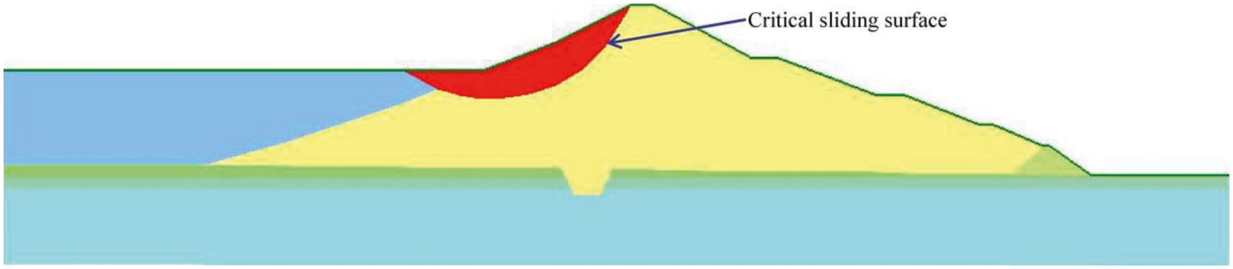
Figure 10: Critical sliding surface of the upstream slope

Figs. 11a–11e show the FS values under the adsorption SWCC for different water level fluctuation rates, where the X axis represents the water level during the fluctuations. The FS initially decreased and then increased during both the water level drawup and drawdown. As a result, the minimum FS occurred during both the water level drawup and drawdown at different critical water levels. In the initial stage of the water level drawup process, the water in the reservoir infiltrated into the lower part of the upstream slope, causing the matrix suction of the lower part to decrease, which manifested as the softening effect in the nearby areas. In this stage, the foot-pressing effect imposed by the water in the reservoir was small, so the softening effect in the lower part was predominant, thus inducing the decrease in the FS. However, in the later stage of the water level drawup, the foot-pressing effect imposed by the water in the reservoir became evident, and the softened area in the lower part of the slope could not develop in a timely manner, which led to an increase in the FS. Comparably, in the initial stage of the water level drawdown, the combined effect of the decrease of the foot-pressing effect imposed by the water in the reservoir and the production of excess pore water pressure in the upper part of the slope induced a decrease in the FS. However, in the later stage of the water level drawdown, the excess pore water pressure dissipated and the shear strength of the upper part of the slope recovered, which gradually dominated the variation in the safety factor of the slope, thus inducing an increase in FS in this stage. Based on Fig. 11, the most dangerous water level, i.e., the critical water level, during the water level drawup was 5 m from the toe of the dam, at 36.9% of the slope height. The most dangerous water level during the water drawdown was 7.5 m from the toe of the dam, at 55.4% of the slope height. An interesting phenomenon is that the critical water levels during both the water level drawup and drawdown were not affected by the water level fluctuation rate. As was reported by Gao et al. [16], the minimum FS of the dam slope was reached before the reservoir was fully drained, which is identical to the results of this study. However, Lane et al. [15] pointed out that the minimum FS is reached when the water level drawdown ratio is 0.8, while it was found to be 0.49 in this study, in which the effective dam height H was defined as the distance from the crest of the dam to the sedimentation elevation. The deviation of the critical drawdown ratio (the ratio of the water level drawdown height to the slope height) may be caused due to the following reasons: (1) the difference in the initial water level before drawdown, which was at the dam crest for Lane and Griffiths’s study but was at an intermediate elevation in this study; and (2) the geological differences between this study and Griffiths’s.

Figure 11: FS of the upstream slope during water level fluctuations under the adsorption SWCC: (a) water level variation rate of 1 m/d; (b) water level variation rate of 2 m/d; (c) water level variation rate of 3 m/d; (d) water level variation rate of 4 m/d; and (e) water level variation rate of 5 m/d

To clarify the reasons for the deviation in the critical drawdown ratio, we reconstructed the FEM model by removing the sludge in the reservoir and set the water level variation from the dam crest to the slope foot, while the other boundary conditions and material properties remained unchanged. The variation in the FS with the water level obtained through simulation is shown in Fig. 12. The variation in the FS is consistent with Fig. 11, showing an increase in the initial stage and a decrease in the subsequent stage, but the critical water level is 15 m. Considering that the total slope height in this case was 32.9 m, we determined that the critical drawdown ratio was about 0.6. By carefully scrutinizing the data of Lane and Griffiths, it was determined that the critical drawdown ratio in the slow drawdown problem is between 0.6 and 0.8. Thus, the minimum FS was reached when the drawdown ratio was 0.6, which is consistent with the results of this study.

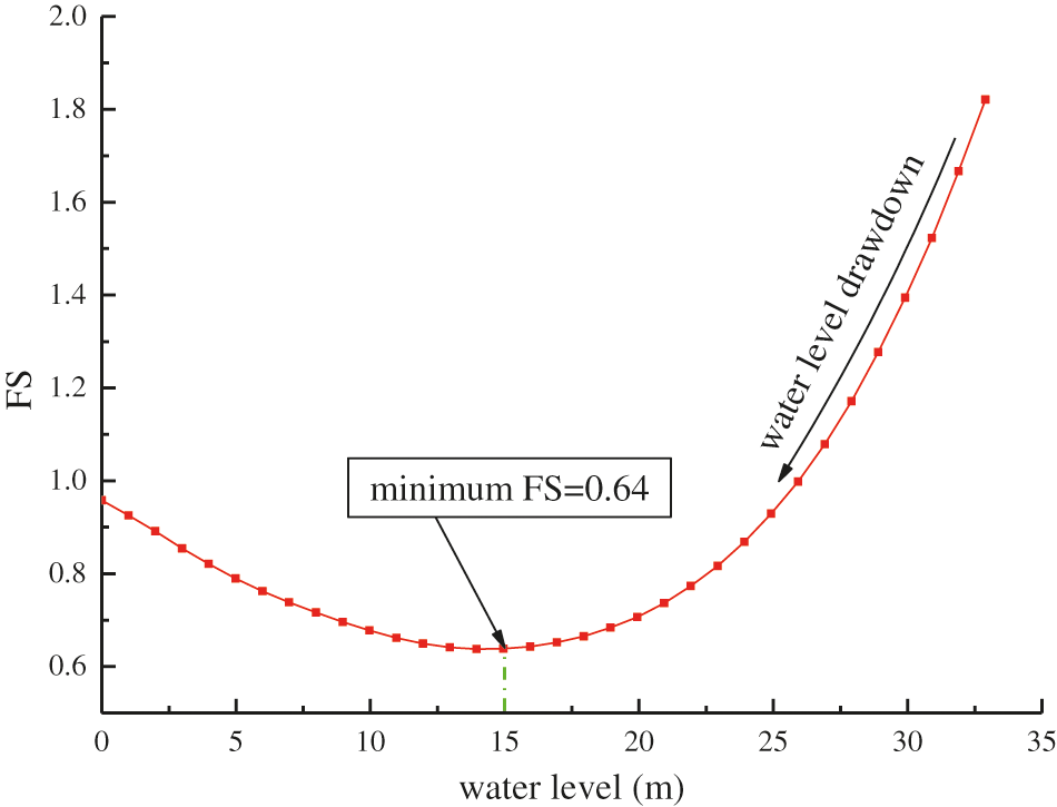
Figure 12: FS variation curve for the upstream dam slope during water level drawdown. This curve is for the situation in which the rate of water level drawdown is 1 m/d, and the sludge in the reservoir has been removed

It should be emphasized that the FS at the beginning of the water level drawup was higher than that of at the end of water level drawdown. The pore water pressure was much lower at the beginning of the water level increase than that at the end of drawdown process due to the dissipation of the excess pore water pressure formed during drawdown continues after the drawdown stopped. This difference in the pore water pressure, which is critical to the slope stability, must cause the different FS values.

Notably, the variation in the FS during the water level drawup did not follow the path of that during the water level drawdown. In addition, it had an approximately identical minimum FS value with a negligible change, while the water level fluctuation rate varied. As a result, in engineering practice, if the minimum FS of the upstream dam slope during a water level drawdown is determined the minimum FS of the water level drawup is also determined, and vice versa. An exciting finding from Fig. 11 is that the FS variation curve under a water level drawup–drawdown cycle intersects, forming three loops: a left incomplete loop, a middle loop, and a right loop. As the water level fluctuation rate increased, the left intersection point moved right, causing the left incomplete loop to enlarge and the middle loop to be squeezed, which can be seen more clearly seen in Fig. 13.

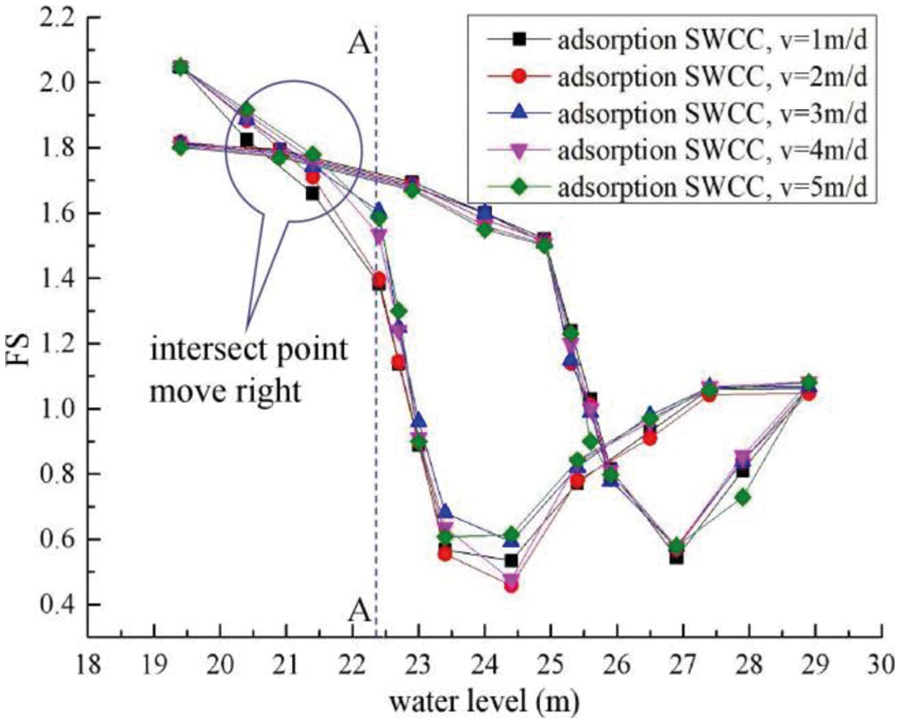
Figure 13: Fs of upstream slope under different water level fluctuation rates

It can be seen from Fig. 13 that the water level fluctuation rate only apparently influenced the water level increase sections of the FS variation curves of water level drawup to the left of line A-A. As the water level fluctuation rate increased, the slopes of these curve sections became more moderate, causing the left intersection point to move to the right. This may be due to the shorter time required for the water to infiltrate into the dam body, while the water level drawup rate increased, which resulted in lower pore water pressures in the dam body.

5.2 Influence of SWCC Hysteresis on the FS under Water Level Fluctuations

As saturated soil mechanics developed, it has been broadly recognized that the matrix suction and the angel of suction friction play important roles in the soil strength [42–44], particularly influencing the stability of soil slopes. In this case, an inevitable factor influencing the dam slope’s stability under water level fluctuations is the SWCC of the soil, which exhibits hysteresis in an adsorption-desorption cycle.

Fig. 14 shows the variation curves of the upstream slope FS with variation in the reservoir’s water level under the hysteresis of the SWCC. It can be seen that in the water level drawup–drawdown cycles the minimum FS of both the water level drawup and drawdown are apparently affected by the SWCC hysteresis, with no other evident difference along the FS variation curves. Through careful scrutiny, the minimum FS of the adsorption SWCC was found to be about 12.38% times higher than that of the desorption SWCC under water level drawup. This could be due to the greater water venting ability of the dam body predicted from the adsorption of the SWCC, causing lower pore water pressures in the dam slope, which is favorable to the stability to the dam slope. Thus, it can be reasonably concluded that the desorption SWCC should be adopted in the assessment of dam slope stability under water level drawup due to its better reliability.

Figure 14: Effect of SWCC hysteresis on the safety factor of the upstream slope: (a) water level variation rate of 1 m/d; (b) water level variation rate of 2 m/d; (c) water level variation rate of 3 m/d; (d) water level variation rate of 4 m/d; and (e) water level variation rate of 5 m/d

Similarly, the minimum FS of the adsorption SWCC is about 41.4% higher than that of the desorption SWCC under water level drawdown. This could be due to the higher permeability derived from the adsorption SWCC letting the water stored in the upstream dam slope swiftly discharge, which is favorable to the dam slope’s stability. As the FS decrease in the initial stage of water level drawdown was mainly caused by the excess pore water pressure in the upstream slope, which depends on the water discharge, the difference between the FS was inevitably maximized at the critical water level, resulting in an evident difference in the minimum FS at this point. In the later stage, the excess pore water pressure dissipated gradually, thus gradually leading to a smaller difference in the FS. In summary, the desorption SWCC should be adopted in the evaluation of upstream dam slope stability under water level fluctuations because it provides a lower critical FS, which is more reliable for assessment. This is consistent with the conclusion of Al-Labban [45].

6  Stability Prediction

Generally, the dam slope stability can be determined through numerical simulation such as the LEM and FEM; however, these methods require a large amount of time. To simplify the calculation process, Gao et al. [16] presented slope stability charts for two dimensional and three dimensional slopes under different water level drawdown conditions, which only consider a simple and homogeneous slope. However, no quick estimation method for FS variation curves of actual dam slopes under water level fluctuations has been developed. As would be expected, if the FS variation curve for water level drawup can be determined, the curve for the water level drawdown can also be determined using a regression operation, and vice versa. This saves a great amount of calculation time and effort.

6.1 Derivation of Equations

Taking Fig. 11 as an example, in Fig. 11a, the FS variation curve for water level drawup can be fitted by a cubic polynomial and by a quadratic polynomial for the sections of the curve with water levels lower than 24.4 m and higher than or equal to 24.4 m, with correlation coefficients (R2) of 0.88584 and 0.99841, respectively.

As Fig. 15 shows, the FS variation curve for a water level drawup rate of 1 m/d can be described by Eq. (30).

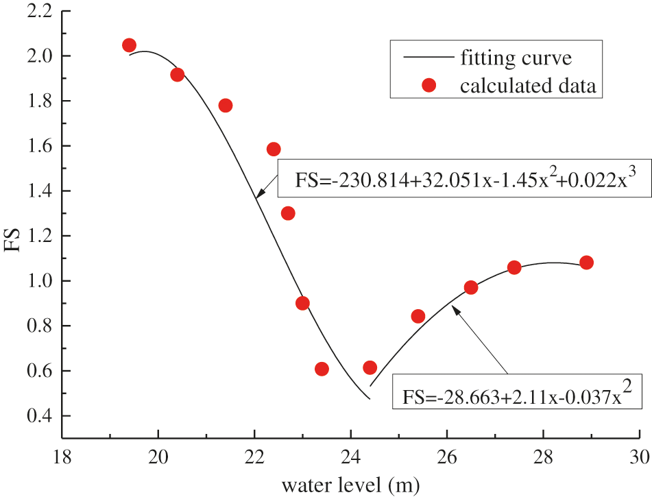
Figure 15: The calculated data and fitting curves for the FS for a water level drawup rate of 1 m/d

{FS=−230.814+32.051x−1.45x2+0.022x3(x<24.4)FS=−28.663+2.11x−0.0373x2(x≥24.4)(30)

As can be seen from Fig. 11, the FS variation curve for water level drawdown can also be fitted using two equations for the sections with water levels lower than or equal to 24.9 m and higher than 24.9 m. Both equations are quadratic polynomials with the same form as Eq. (31) and require three parameters to be determined.

FS=ax2+bx+c,(31)

where a, b, and c are undetermined coefficients, which can be determined from the coordinates of points A, B, C, D, E, and F in Fig. 11a using the regression method. First, the coordinates of points A, B, and C, through which the FS variation curves for the water level drawdown inevitably passes, can be obtained using Eq. (30). The coordinates of the three points are (28.9, 1.072), (26.9, 0.544), and (25.9, 0.816), respectively. Using the regression method, the FS variation equation for water levels higher than 24.9 m during drawdown is Eq. (32).

FS=0.179x2−9.71x+132.34(x≥24.9)(32)

Then, by substituting x = 24.9 into Eq. (32), the coordinates of point D can be obtained, i.e., (24.9, 1.54). Furthermore, from Fig. 11, the x coordinate of point E can be derived as a function of the water level fluctuation rate using the regression method:

xE=20.128+0.466V−0.034V2.(33)

Since point E is the intersection point of the FS variation curves for water level drawup and drawdown, the y coordinate of point E on the FS variation curve for water level drawdown can be obtained by substituting Eq. (33) into the first function of Eq. (30) as follows:

FS(E)=−230.814+32.051xE−1.45xE2+0.022xE3.(34)

In the current case study, v was equal to 1 m/d, producing an xE value of 20.56 through Eq. (33). By substituting this value into Eq. (34), the FS(E) value of 1.95 was obtained. Thus, the coordinates of point E are (20.56, 1.95). Additionally, the FS variation curves for water level drawdown in Fig. 11 constantly pass through point F, which has coordinates of (19.4, 1.81).

Through regression analysis of the coordinates of points D, E, and F, the FS variation curve for water level drawdown for water levels of lower than 24.9 m can be derived using Eq. (35).

FS=−15.184+1.655x−0.039x2(x<24.9).(35)

By combining Eqs. (32) and (35), the complete equation for predicting the FS variation curve for water level drawdown can be derived (Eq. (36)). It should be noted that point E moves to the right as the water level variation rate increases, inducing different equations for the FS variation. Eq. (36) is for a water level drawdown rate of 1 m/d and simply provides an example.

{FS=0.179x2−9.71x+132.34(x≥24.9)FS=−0.039x2+1.655x−15.184(x<24.9)(36)

6.2 Equations Validation

To validate the accuracy of the prediction equation (Eq. (36)), six calculated points were selected for comparison with the corresponding predicted values. As is shown in Fig. 16, the calculated values are close to the predicted curve, with relative errors of 2.1%–14.4%. It is reasonably concluded that the derived prediction equation (Eq. (36)) for the variation in the FS with water level can be used to approximate the stability of the up-stream dam slope during water level drawdown.

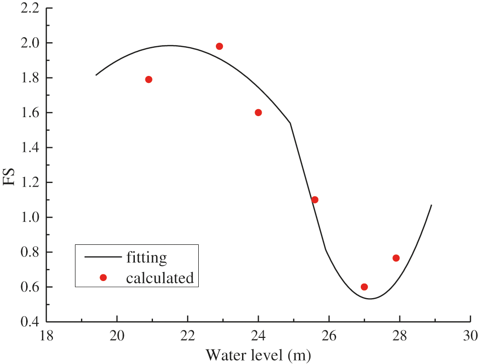
Figure 16: The predicted FS variation curve for water level drawdown

7  Conclusions

Dam slope collapse events have occurred worldwide under water level fluctuations and have caused numerous casualties to the people living nearby and thus studying dam slope stability under water level drawup and drawdown is of great importance. Based on an actual dam, the effects of the water level fluctuation rate and the hysteresis of the SWCC on the FS of the dam slope were studied via numerical simulations. Based on the calculation results, the following conclusions were drawn:

1.    The free surface in the dam body for the desorption SWCC during water level fluctuations was higher than that for the adsorption SWCC, which would be more evident at higher water levels.

2.    The FS of the upstream dam slope under water level drawup initially decreased and then increased, with the minimum value occurring at a reservoir water level of about 36.9% of the slope height, which is referred to as the critical water level.

3.    Similarly, the FS of the upstream dam slope initially decreased and then increased, with a critical reservoir water level of around 55.4% of the slope height during water level drawdown. The FS variation curve did not follow that of the water level drawup; however, it had a minimum FS value identical to that for water level drawup.

4.    The critical water levels during both water level drawup and drawdown were not affected by the water level fluctuation rate and the SWCC hysteresis.

5.    The minimum FS of both the water level drawup and drawdown were apparently affected by the SWCC hysteresis. The minimum FS of the adsorption SWCC was higher than that of the desorption SWCC under both water level drawup and drawdown. Consequently, it is advised that the desorption SWCC be used in engineering practice for the sake of reliability.

6.    Under the circumstance of a determined FS variation curve for water level drawup, a method using a prediction equation was derived to quickly estimate the FS variation curve for water level drawdown. It has application value regarding controlling dam slope stability during water level drawdown for dam structures identical to that analyzed in this study.

Acknowledgement: This study was directed by professor Zhou Zhijun of Changan University, China, and was attributed to the cooperation of Ye Wanjun’s researching team in Xi’an University of Science and Technology, China.

Funding Statement: This research was funded by the Key R&D Program of Science and Technology Bureau of Shangluo City (Grant No. 2020-Z-0111) and Scientific Research Program of Science and Technology Department of Shaanxi Province (Grant No. 2021JQ-844).

Conflicts of Interest: The authors declare that they have no conflicts of interest to report regarding the present study.

References

 1.  Hiroyuki, N. (1990). Reservoir landslide. Bulletin of Soil and Water Conservation, 10(1), 53–64. [Google Scholar]

 2.  Zhong, L. (1994). Enlightenments from the accident of Vaiont landslide in Italy. The Chinese Journal of Geological Hazard and Control, 5(2), 77–84 (in Chinese). DOI 10.16031/j.cnki.issn.1003-8035.1994.02.012. [Google Scholar] [CrossRef]

 3.  Zhang, W., Zhan, L., Ling, D., Chen, Y. (2006). Influence of reservoir water level fluctuations on stability of unsaturated soil banks. Journal of ZheJiang University (Engineering Science), 40(8), 1365–1428. DOI 10.1016/S0379-4172(06)60085-1. [Google Scholar] [CrossRef]

 4.  Mehmet, M. B. (2007). Investigation of stability of slopes under drawdown conditions. Computers and Geotechnics, 34(4), 81–91. DOI 10.1016/j.compgeo.2006.10.004. [Google Scholar] [CrossRef]

 5.  Anilan, T., Nacar, S., Kankal, M., Yuksek, O. (2020). Prediction of maximum annual flood discharges using artificial neural network approaches. Gradevinar, 72(3), 215–224. DOI 10.14256/JCE.2316.2018. [Google Scholar] [CrossRef]

 6.  Zheng, S., Jiang, A. N., Feng, K. S. (2021). A reliability evaluation method for intermittent jointed rock slope based on evolutionary support vector machine. Computer Modeling in Engineering & Sciences, 129(1), 149–166. DOI 10.32604/cmes.2021.016761. [Google Scholar] [CrossRef]

 7.  Rezaeeian, A., Davoodi, M., Jafari, M. K. (2019). Determination of optimum cross section of earth dams using ant colony optimization algorithm. Scientia Iranica, 26(3), 1104–1121. DOI 10.24200/sci.2018.21078. [Google Scholar] [CrossRef]

 8.  Morgernstern, N. R. (1963). Stability charts for earth slopes during rapid drawdown. Geotechnique, 13(2), 121–131. DOI 10.1680/geot.1963.13.2.121. [Google Scholar] [CrossRef]

 9.  Desai, C. S. (1977). Drawdown analysis of slopes by numerical method. Journal of Geotechnical and Geoenvironmental Engineering, 103(7), 667–676. DOI 10.1016/0022-1694(77)90030-0. [Google Scholar] [CrossRef]

10. Jiang, Q., Tang, Y. A. (2015). General approximate method for the groundwater response problem caused by water level variation. Journal of Hydrology, 529(7), 398–409. DOI 10.1016/j.jhydrol.2015.07.030. [Google Scholar] [CrossRef]

11. Jiang, Q., Ye, Z., Zhou, C. (2014). A numerical procedure for transient free surface seepage through fracture networks. Journal of Hydrology, 519(7), 881–891. DOI 10.1016/j.jhydrol.2014.07.066. [Google Scholar] [CrossRef]

12. Sun, G., Zheng, H., Tang, H., Dai, F. (2016). Huangtupo landslide stability under water level fluctuations of the Three Gorges reservoir. Landslides, 13(5), 1167–1179. DOI 10.1007/s10346-015-0637-7. [Google Scholar] [CrossRef]

13. Zheng, Y., Shi, W., Kong, W. (2004). Calculation of seepage forces and phreatic surface under drawdown conditions. Chinese Journal of Rock Mechanics and Engineering, 23(18), 3203–3210 (in Chinese). DOI 10.1097/00004836-200411000-00015. [Google Scholar] [CrossRef]

14. Griffiths, D. V., Lane, P. A. (1999). Slope stability analysis by finite elements. Geotechnique, 49(3), 387–403. DOI 10.1680/geot.1999.49.3.387. [Google Scholar] [CrossRef]

15. Lane, P. A., Griffiths, D. V. (2000). Assessment of stability of slopes under drawdown conditions. Journal of Geotechnical and Geoenvironmental Engineering, 126(5), 443–450. DOI 10.1061/(ASCE)1090-0241(2000)126:5(443). [Google Scholar] [CrossRef]

16. Gao, Y., Zhu, D., Zhang, F., Lei, G. H., Qin, H. (2014). Stability analysis of three-dimensional slopes under water drawdown conditions. Canadian Geotechnical Journal, 51(11), 1355–1364. DOI 10.1139/cgj-2013-0448. [Google Scholar] [CrossRef]

17. Fredlund, D. G., Morgenstern, N. R., Widger, R. A. (1978). The shear strength of unsaturated soils. Canadian Geotechnical Journal, 15(3), 313–321. DOI 10.1139/t78-029. [Google Scholar] [CrossRef]

18. Nuria, M. P., Eduardo, E. A., Sebastia, O. (2008). Rapid drawdown in slopes and embankments. Water Resources Research, 44(5), W00D03. DOI 10.1029/2007WR006525. [Google Scholar] [CrossRef]

19. Wang, L., Wu, C., Gu, X., Liu, H., Mei, G. et al. (2020). Probabilistic stability analysis of earth dam slope under transient seepage using multivariate adaptive regression splines. Bulletin of Engineering Geology and the Environment, 79(6), 2763–2775. DOI 10.1007/s10064-020-01730-0. [Google Scholar] [CrossRef]

20. Sun, G., Yang, Y., Cheng, S., Zheng, H. (2017). Phreatic line calculation and stability analysis of slopes under the combined effect of reservoir water level fluctuations and rainfall. Canadian Geotechnical Journal, 54(5), 631–645. DOI 10.1139/cgj-2016-0315. [Google Scholar] [CrossRef]

21. Wang, L., Wu, J., Zhang, W., Wang, L., Cui, W. (2021). Efficient seismic stability analysis of embankment slopes subjected to water level changes using gradient boosting algorithms. Frontiers in Earth Science, 9, 807317. DOI 10.3389/feart.2021.807317. [Google Scholar] [CrossRef]

22. Biswas, N., Chakraborty, S., Mosadegh, L., Puppala, A. J., Corcoran, M. (2020). Influence of anisotropic permeability on slope stability analysis of an earthen dam during rapid drawdown. Geo-Congress 2020: Engineering, Monitoring, and Management of Geotechnical Infrastructure, 316, 29–39. DOI 10.1061/9780784482797. [Google Scholar] [CrossRef]

23. Yu, S., Ren, X., Zhang, J., Wang, H., Wang, J. et al. (2020). Seepage, deformation, and stability analysis of sandy and clay slopes with different permeability anisotropy characteristics affected by reservoir water level fluctuations. Water, 12(1), 1–14. DOI 10.3390/w12010201. [Google Scholar] [CrossRef]

24. Jiang, S. H., Liu, X., Huang, J. (2020). Non-intrusive reliability analysis of unsaturated embankment slopes accounting for spatial variabilities of soil hydraulic and shear strength parameters. Engineering with Computers, 36(7), 1–14. DOI 10.1007/s00366-020-01108-6. [Google Scholar] [CrossRef]

25. Kayabasi, A. (2020). Evaluation of a reservoir landslide: A case study from Artvin, Turkey. Arabian Journal of Geosciences, 13(2), 1–17. DOI 10.1007/s12517-019-5021-9. [Google Scholar] [CrossRef]

26. Ibanez, J. P., Hatzor, Y. H. (2018). Rapid sliding and friction degradation: Lessons from the catastrophic Vajont landslide. Engineering Geology, 244(1), 96–106. DOI 10.1016/j.enggeo.2018.07.029. [Google Scholar] [CrossRef]

27. Michoud, C., Baumann, V., Lauknes, T. R., Penna, I., Derron, M. H. et al. (2016). Large slope deformations detection and monitoring along shores of the Potrerillos dam reservoir, Argentina, based on a small-baseline InSAR approach. Landslides, 13(3), 451–465. DOI 10.1007/s10346-015-0583-4. [Google Scholar] [CrossRef]

28. Saroli, M., Stramondo, S., Moro, M., Doumaz, F. (2005). Movements detection of deep seated gravitational slope deformations by means of InSAR data and photogeological interpretation: Northern Sicily case study. Terra Nova, 17(1), 35–43. DOI 10.1111/j.1365-3121.2004.00581.x. [Google Scholar] [CrossRef]

29. Kanik, M., Ersoy, H. (2019). Evaluation of the engineering geological investigation of the Ayvali dam site (NE Turkey). Arabian Journal of Geosciences, 12(3), 89. DOI 10.1007/s12517-019-4243-1. [Google Scholar] [CrossRef]

30. Xiong, X., Shi, Z., Xiong, Y., Peng, M., Ma, X. et al. (2019). Unsaturated slope stability around the Three Gorges Reservoir under various combinations of rainfall and water level fluctuation. Engineering Geology, 261(5), 1–17. DOI 10.1016/j.enggeo.2019.105231. [Google Scholar] [CrossRef]

31. Xiong, X., Shi, Z. M., Guan, S. G., Zhang, F. (2018). Failure mechanism of unsaturated landslide dam under seepage loading-Model tests and corresponding numerical simulations. Soils and Foundations, 58(5), 1133–1152. DOI 10.1016/j.sandf.2018.05.012. [Google Scholar] [CrossRef]

32. Miao, F., Wu, Y., Li, L., Tang, H., Li, Y. (2018). Centrifuge model test on the retrogressive landslide subjected to reservoir water level fluctuation. Engineering Geology, 245(1), 169–179. DOI 10.1016/j.enggeo.2018.08.016. [Google Scholar] [CrossRef]

33. Sadeghi, S., Hakimzadeh, H., Babaeian Amini, A. (2020). Experimental investigation into outflow hydrographs of nonhomogeneous earth dam breaching due to overtopping. Journal of Hydraulic Engineering, 146(1), 04019049-1–04019049-12. DOI 10.1061/(ASCE)HY.1943-7900.0001664. [Google Scholar] [CrossRef]

34. Kakinuma, T., Shimizu, Y. (2014). Large-scale experiment and numerical modeling of a riverine levee breach. Journal of Hydraulic Engineering, 140(9), 4014039-1–4014039-9. DOI 10.1061/(ASCE)HY.1943-7900.0000902. [Google Scholar] [CrossRef]

35. Duncan, J. M. (1996). State of the art: limit equilibrium and finite-element analysis of slopes. Journal of Geotechnical Engineering, 122(7), 577–596. DOI 10.1061/(ASCE)0733-9410(1996)122:7(577). [Google Scholar] [CrossRef]

36. Dawson, E. M., Roth, W. H., Drescher, A. (1999). Slope stability analysis by strength reduction. Geotechnique, 49(6), 835–840. DOI 10.1680/geot.1999.49.6.835. [Google Scholar] [CrossRef]

37. Li, D. Q., Xiao, T., Cao, Z. J., Zhou, C. B., Zhang, L. M. (2016). Enhancement of random finite element method in reliability analysis and risk assessment of soil slopes using Subset Simulation. Landslides, 13(2), 293–303. DOI 10.1007/s10346-015-0569-2. [Google Scholar] [CrossRef]

38. Liang, C., Jaksa, M. B., Ostendorf, B., Kuo, Y. L. (2015). Influence of river level fluctuations and climate on riverbank stability. Computers and Geotechnics, 63(4), 83–98. DOI 10.1016/j.compgeo.2014.08.012. [Google Scholar] [CrossRef]

39. Liu, L., Zhang, S., Cheng, Y. M., Liang, L. (2019). Advanced reliability analysis of slopes in spatially variable soils using multivariate adaptive regression splines. Geoscience Frontiers, 10(2), 671–682. DOI 10.1016/j.gsf.2018.03.013. [Google Scholar] [CrossRef]

40. Van Genuchten, M. T. (1980). A closed-form equation for predicting the hydraulic conductivity of unsaturated soils. Soil Science Society of America Journal, 44(5), 892–898. DOI 10.2136/sssaj1980.03615995004400050002x. [Google Scholar] [CrossRef]

41. Siegel, R. A., Kovacs, W. D., Lovell, C. W. (1981). Random surface generation in stability analysis. Journal of the Geotechnical Engineering Division, 107(7), 996–1002. DOI 10.1061/AJGEB6.0001409. [Google Scholar] [CrossRef]

42. Fredlund, D. G., Rahardjo, H. (1993). Soil mechanics for unsaturated soils (First Edition). New York: Wiley Interscience Press. [Google Scholar]

43. Aqtash, U. A., Bandini, P. (2015). Prediction of unsaturated shear strength of an adobe soil from the soil-water characteristic curve. Construction and Building Materials, 98(4), 892–899. DOI 10.1016/j.conbuildmat.2015.07.188. [Google Scholar] [CrossRef]

44. Vanapalli, S. K., Fredlund, D. G., Pufahl, D. E., Clifton, A. W. (1996). Model for the prediction of shear strength with respect to soil suction. Canadian Geotechnical Journal, 33(3), 379–392. DOI 10.1139/t96-060. [Google Scholar] [CrossRef]

45. Al-Labban, S. (2018). Seepage and stability analysis of the earth dams under drawdown conditions by using the finite element method (Ph.D. Thesis). University of Central Florida, Florida. [Google Scholar]

This work is licensed under a Creative Commons Attribution 4.0 International License, which permits unrestricted use, distribution, and reproduction in any medium, provided the original work is properly cited.