Computer Modeling in Engineering & Sciences

---

DOI: 10.32604/cmes.2022.020601

REVIEW

Advances in Hyperspectral Image Classification Based on Convolutional Neural Networks: A Review

Somenath Bera1, Vimal K. Shrivastava2 and Suresh Chandra Satapathy3,*

1School of Computer Science and Engineering, Lovely Professional University, Phagwara, 144411, India
2School of Electronics Engineering, Kalinga Institute of Industrial Technology (KIIT), Bhubaneswar, 751024, India
3School of Computer Engineering, Kalinga Institute of Industrial Technology (KIIT), Bhubaneswar, 751024, India
*Corresponding Author: Suresh Chandra Satapathy. Email: suresh.satapathyfcs@kiit.ac.in
Received: 02 December 2021; Accepted: 16 March 2022

1  Introduction

Hyperspectral imaging, also known as imaging spectroscopy, records hundreds of continuous and narrow spectral bands in the range of visible light to infrared spectrum and generate hyperspectral image (HSI) [1]. It contains both spectral and spatial information about the objects and can be visualized as a data cube. A representation of HSI is shown in Fig. 1, where each spectral band represents an image with a particular wavelength. A pixel in HSI can be represented with a wide range of spectral values and is surrounded by neighboring pixels. The set of values in the spectral domain provides the spectral information whereas neighboring pixels offer spatial information. With such rich spectral and spatial information, HSIs have been applied in many fields, such as mineralogy [2], surveillance [3], physics [4], astronomy [5], chemical imaging [6], military [7], agriculture [8], environment monitoring [9], and so on. The main task in these applications is classification of pixels to identify the objects.

Figure 1: Representation of HSI

To classify the HSI pixels, several classification methods such as support vector machine (SVM) [10,11], distance measure [12,13], k-nearest neighbors (KNN) [14,15], maximum likelihood criterion [16,17] and logistic regression [18,19], have been applied in the past. The performance of these methods was not satisfactory due to the consideration of spectral information alone. Therefore, many classification methods have been proposed to improve the performance by incorporating spatial information [20–23]. The spatial information provides shape and size of the objects. With the help of spectral and spatial information, several methods improved the classification accuracy but failed to generate smooth classification maps due to their shallow learning nature.

Recently, deep learning [24–29] has been considered as the state-of-the-art machine learning technique [30,31]. It automatically learns hierarchical features from raw input and has made great breakthrough in various domains viz. computer vision [32], object detection [33], medical imaging [34], agriculture [35], and natural language processing [36,37], etc. Motivated by these successful applications, deep learning concept has also been introduced in HSI classification and demonstrated good performance [38]. Many deep learning models were applied in HSI classification such as stacked autoencoder (SAE) [39,40], deep belief network (DBN) [41,42], and convolutional neural network (CNN) [43–48]. Among these models, DBN and SAE are unsupervised learning and does not require labeled samples for training. However, the main problem of SAE and DBN lies in the initial stage, where images are flattened into vectors to fulfill the input requirement, which leads to spatial information loss. Compared with SAE and DBN, CNN is very efficient for extracting spectral-spatial information and significantly improves the classification performance [49]. Beside this, CNN has shown its effectiveness in normal image classification [50,51]. Guo et al. [52] proposed an attention network, where 2D CNN was utilized as spatial feature extraction and 3D CNN as spectral-spatial feature extraction tools for HSI classification. In [53], authors have introduced graph CNN due to its powerful representation ability and achieved impressive performance. Moreover, many recent HSI classification methods have introduced feature fusion techniques to improve the classification performance [54]. Ge et al. [55] proposed a fusion based method, where 2D CNN and 3D CNN were combined to extract abstract spatial features and multi-branch network was employed for exploiting features at different levels.

In the last few years, many review articles have been published based on HSI classification [56–58]. For instance, Ma et al. [59] presented a review of how deep learning has been applied in remote sensing image analysis and can be an effective tool in future. In [60], Gewali et al. reviewed several literatures related to machine learning algorithm and hyperspectral image analysis. Authors further compared different machine learning based hyperspectral image analysis methods to address the critical challenges. In [61], authors concentrated on the basics of HSI analysis and their various applications. Ghamisi et al. [62] presented a detailed discussion about spectral information based HSI classification methods. He et al. [63] focused on spectral-spatial analysis of HSI by using a spatial dependency concept. In [64], Li et al. systematically reviewed the deep learning based HSI classification methods and introduced few strategies to address the limited samples problems. From these literature, we have observed that many review articles have been presented on HSI classification in a generalized way. However, none of the review articles have provided detailed analysis on CNN based HSI classification that has produced most prominent results on HSI classification. Therefore, we have specifically focused on CNN based HSI classification by presenting a deep and systematic analysis. To accomplish this, we have divided the literature into four groups that include spectral-based CNN methods, spatial-based CNN methods, spectral-spatial based CNN methods and fusion based CNN methods. Then, comprehensive review has been performed on these methods. Further, a detailed comparative analysis has been presented between four CNN based models namely 1D CNN, 2D CNN, 3D CNN, and feature fusion based CNN (FFCNN) on four HSI datasets. Lastly, challenges and future guidelines have been provided.

The remainder of this paper is organized as follows. Section 2 makes a brief introduction to CNN and its different architectures. Section 3 reviews the previous work into four aspects based on the types of features utilized by different CNN architectures. The architectural details of four CNN based models have been discussed in Section 4. Section 5 provides the comparative performance analysis of four models on four HSI datasets. Conclusions and future guidelines are provided in Section 6.

2  Overview of CNN Architecture

The working principal of CNN was inspired by the neuroscience. The neuroscience defines how a different level of processing can help in recognizing the objects [65]. To identify the object, CNN takes the advantage of two special characteristics: local connection and shared weights. The local connection is used to extract the spatial features and shared weights reduce the network parameters [66]. In Fig. 2, a general CNN based model is presented that contains convolutional, pooling and fully connected layers. From the figure, we can see that the convolutional and pooling layers are stacked alternately to extract the deep features followed by fully connected layer. The details of each layer are discussed below:

The convolutional layer is characterized by the set of kernels and biases. These kernels have a small receptive field and are used for extracting specific features. More specifically, a kernel is used for generating the feature map. A feature map of the convolutional layer can be defined as follows:

fjl=∑i=1Tα(fil−1∗wijl+bil)(1)

where fjl represents jth feature map of the current lth layer, fil−1 is the ith feature map of the previous (l−1)th layer and T is the number of bands. wijl and bil are weight and bias. The * operator is used for convolution operation and α denotes the activation function. In CNN, a pooling layer is added after each convolutional layer to reduce the size of the feature maps without losing discriminative information. Further, it provides translation invariant property. After several convolutional and pooling layers, the feature maps are flattened into one dimensional vector and input to fully connected layer. The number of neurons in the last fully connected layer is equal to the number of classes. The softmax function is used at the last layer, which is a logistic regression function for generating the probability distribution of classes.

Figure 2: General architecture of convolutional neural network

2.1 Types of CNN

A CNN architecture is categorized based on application domain of convolution operation. Specifically, when a convolutional operation is conducted on spectral domain of input data, the CNN is called 1D CNN [67]. In 1D CNN, the neuron’s value nija at position a in the jth feature map of ith layer can be represented as follows:

nija=α(∑k∑r=0Ri−1n(i−1)ka+r∗wijkr+bij)(2)

where k denotes the (i−1)th layer’s feature map which is connected with the current feature map, wijkr is the weight at position r connected to the kth feature map, bij is the bias of jth feature map in the ith layer, Ri is the width of the kernel to the spectral dimension. Similarly, when convolution operation is conducted on spatial and spectral-spatial domains, it is called 2D CNN [68] and 3D CNN [69], respectively. The neuron’s value n of the jth feature map in ith layer for 2D CNN and 3D CNN are represented in (3) and (4), respectively.

nijab=α(∑k∑r=0Ri−1∑s=0Si−1n(i−1)k(a+r)(b+s)∗wijkrs+bij)(3)

nijabc=α(∑k∑r=0Ri−1∑s=0Si−1∑t=0Ti−1n(i−1)k(a+r)(b+s)(c+t)∗wijkrst+bij)(4)

where Si is the height of the convolutional kernel, Ti is the size of the kernel with respect to spectral dimension.

3  CNN Based HSI Classification Methods

CNN has the power to extract discriminative features from complex hyperspectral data. With the help of discriminative features, CNN based methods can efficiently identify the ground objects [70,71]. A large number of CNN based methods have been developed for HSI classification in last few years and achieved state-of-the-art performance [72–75]. We have divided the literature into four groups that include spectral-based CNN methods, spatial-based CNN methods, spectral-spatial based CNN methods and fusion based CNN methods.

3.1 Spectral Based CNN Methods

One of the most important properties of HSI is spectral information which helps to identify small objects [76–78]. To get the spectral information, 1D CNN plays an important role in HSI community. Many methods have been proposed for extracting spectral information. Among them, 1D CNN shows efficiency with the advantage of conceptual simplicity and ease of implementation [68]. For example, Chen et al. [79] proposed a CNN based model for HSI classification, which was designed automatically and fitted well to specific datasets. Specifically, the model uses 1D Auto-CNN for classifying HSI. In [80], authors explored the power of 1D CNN to extract spectral features and demonstrated good performance than traditional methods. Recently, Sun et al. [81] adopted CNN to exploit localized spectral features from several band groups. Although, spectral information improves the classification performance but fails to describe the structure of an object.

3.2 Spatial Based CNN Methods

Spatial information is another important information resource of HSI, which can be used to represent the shape and size of the objects. As CNN has got huge popularity for extracting spatial information in various fields [82,83], many methods have incorporated spatial information into their models and reported improved classification accuracy over the past decades [84–87]. In [88], spatial features extracted by multiscale CNN were integrated with spectral features achieved by long short-term memory (LSTM) to accomplish the HSI classification. Yue et al. [66] introduced a deep CNN model to extract spatial features with the help of Principal Component Analysis (PCA) [89,90] and logistic regression. Xu et al. [91] integrated HSI data and multiple sensor’s data for improving the classification performance, where spectral and spatial features of HSI data were extracted through 1D CNN and 2D CNN, respectively. In addition, several literature used off-the-shelf CNN models including AlexNet [43], VGGNet [92], GoogLeNet [93] and ResNet [94] for deep spatial feature extraction on HSI datasets and achieved high classification accuracy. In more detail, Cheng et al. [95] proposed a classification framework, where spatial features were exploited through off-the-shelf CNN models and improved performance has been obtained by metric learning based approach. In [96], spatial features exploited through 2D CNN were combined with spectral features to enhance the classification performance. Makantasis et al. [97] employed CNN to encode the spatial information of pixels followed by Multi-Layer perception. In [98], authors extracted deep spatial features by CNN and their characteristics have been investigated by sparse representation based framework. Moreover, in our previous works, we have analyzed the effect of various pooling strategies [99] and optimizers [100] on the performance of 2D CNN based HSI classification system. It has been observed that though the utilization of spatial information can enhance the representation power of HSI but unable to fully identify the small objects.

3.3 Spectral-Spatial Based CNN Methods

Considering only spectral or spatial information of HSI is not enough for improving the classification performance [101–103]. Both spectral and spatial information are essential [63,104,105]. Studies report that joint spectral-spatial based methods significantly improve the classification results [106–113]. During the last few years, 3D CNN has got huge popularity for extracting joint spectral-spatial features and shown remarkable performance in HSI classification [114]. Li et al. [69] presented a CNN model that jointly extracts spectral-spatial features from HSI dataset without depending on pre-processing and post-processing task [67]. Mei et al. [115] integrated the spectral and spatial features by constructing five layer CNN model with regularization technique. Liu et al. [116] proposed a 3D CNN based classification model to simultaneously learn spectral-spatial features and adopted virtual sample concept to address the limited training sample problem. In [117], joint spectral-spatial features were exploited through CNN based multi-feature learning model. Shi et al. [118] proposed a HSI classification model as a combination of CNN and multi-resolution analysis to extract 3D features. Zhu et al. [119] designed a deep 3D Capsule framework for spectral-spatial classification. Zou et al. [120] exploited joint spectral-spatial and semantic information by 3D fully convolutional network to boost the classification accuracy. In [105], the proposed model not only extracted spectral-spatial features but also minimized the computational cost. Roy et al. [121] adopted hybrid CNN model to maintain the classification accuracy. In [80], Chen et al. introduced 3D CNN to simultaneously learn the deep spectral and spatial features. However, there may be loss of spectral information when spectral-spatial features were extracted jointly due to the involvement of convolution operation on non-informative spectral bands [88]. Therefore, separate spectral and spatial feature extraction and their fusion may be an alternative choice to better utilize the spectral and spatial information in HSI classification.

3.4 Fusion Based CNN Methods

Feature fusion concept is another important step in HSI classification for better utilizing the spectral and spatial information [54,122]. The feature fusion can help in extracting the abstract features and improve the classification performance [123–127]. It also helps in merging the detailed and boundary information of shallow layers and semantic information of deep layers [128]. Many literature have fused the spectral and spatial features in different manner and have shown better classification accuracy [49,91,129,130]. Kang et al. [131] proposed a novel fusion scheme where group of adjacent bands were fused by averaging and processed with recursive filtering to get the resulting features for classification. In [132], Guo et al. introduced fusion method for HSI classification, where CNN and guided filter have been adopted for spectral and multiscale spatial feature extraction, respectively. In [133], a multilayer feature fusion based triple-architecture CNN has been presented, where spectral and spatial features were extracted by stacking of spectral features to dual-scale spatial features with sample augmentation using local and non-local constrains. In [134], spectral and spatial features were extracted through balanced local discriminate embedding and CNN, respectively to construct the fused features. Gao et al. [135] employed CNN to construct fusion network by adopting multi-branch concepts. In [136], spatial based deep CNN architecture was integrated with pixel based shallow structured multilayer perception by utilizing decision fusion approach for classifying fine resolution remotely sensed data. Liang et al. [137] introduced a novel feature fusion method where multiscale deep spatial features were extracted through VGG16 model and spectral features were exploited directly. Then, spectral and spatial features were fused with the help of unsupervised sparse autoencoder. In [138], authors used CNN based information fusion network for combining heterogeneous information of HSI and light detection and ranging (LiDAR) data and achieved state-of-the-art results. From these fusion techniques, it has been observed that fusion can improve the classification performance of HSI.

4  HSI Classification Framework Using CNN

We have presented a comparative performance analysis on HSI classification using four CNN based models (namely 1D CNN, 2D CNN, 3D CNN, and FFCNN) based on their specific feature extraction capabilities. Specifically, 1D CNN, 2D CNN, 3D CNN, and FFCNN are based on spectral, spatial, spectral-spatial, and feature fusion, respectively. Moreover, the architecture of those four CNN models have been introduced and discussed in the following subsections.

4.1 Spectral Based 1D CNN

A pixel in HSI is represented by set of spectral values with particular wavelength. These values offer spectral information to identify small objects. As shown in Fig. 3, a 1D CNN based model is built to extract spectral information by considering entire spectral bands of HSI. In addition, the model uses several convolutional and pooling layers to extract the deep spectral information followed by fully connected layer to exploit the more abstract information.

Figure 3: Architecture of 1D CNN model for spectral feture extraction

4.2 Spatial Based 2D CNN

In HSI, spatial information of a pixel is captured from the neighboring pixels. The spatial information helps in describing the shape and size of the objects. As shown in Fig. 4, a 2D CNN based model is constructed for extracting spatial information. The PCA has been employed to select single band as principal component followed by patch extraction. The model then applies many convolutional and pooling operations on extracted patches to get the spatial information.

Figure 4: Architecture of 2D CNN model for spatial feture extraction

4.3 Spectral Spatial Based 3D CNN

Only spectral or spatial information is not enough for identifying the ground objects of HSI. Both spectral and spatial information play a vital role in HSI classification. As shown in Fig. 5, a model has been built, which utilizes both spectral and spatial information of HSI. The model uses only a few informative bands by selecting the first few principal components (bands). Then, patch extraction is done followed by joint spectral-spatial feature extraction.

Figure 5: Architecture of 3D CNN model for spectral-spatial feature extraction

4.4 FFCNN

Recently, feature fusion technique is very popular in HSI classification. As shown in Fig. 6, we have designed a model named FFCNN, where spectral and spatial information are fused to increase the representation of HSI. In this model, the spectral and spatial information are extracted separately through 1D CNN and 3D CNN, respectively to reduce the information loss. Finally, the spectral and spatial features were fused before fully connected layer.

Figure 6: Architecture of FFCNN model for feature fusion

From 3 to 6, we can observe that four models are presented for HSI classification. In order to classify HSI, some preprocessing steps have been taken for each model. Initially, HSI is normalized in the range of −0.5 to +0.5 before applying PCA. The PCA is used for selecting the most informative band(s). For 1D CNN, inputs are prepared by directly extracting the pixel vectors from HSI datasets. For the other models, image patches of size 27 × 27 [80] are cropped from the band(s) and considered as inputs. After preparing the different structured inputs xs, the output of the models can be computed as follows:

ys=f(xs∗W+B),s=1,2,…S.(5)

where f denotes the composite function for input, which is obtained after applying several linear and nonlinear operations. W and B represent the weight and bias of the model, respectively and S is the number of training samples. A softmax function is used to generate the probability distribution of each output and can be represented as follows:

pis=eyis∑j=1Teyjs,i=1,2,…T.(6)

where yis is the ith value of y sand T is the number of classes. Depending on the true and predicted values, the cost function L is defined as follows:

L=−1S∑s=1S⁡[tilogpi+(1−ti)log(1−pi)](7)

where ti and pi are the true and predicted label of ith data, respectively. To reduce the cost function, the Adam optimizer [100] has been adopted. After completing the optimization [139], the models are ready to predict the class label of test samples x′ depending on maximum probability pi.

Class(x′)=argmaxpi,i=1,2,…,T.(8)

5  Results and Discussion

5.1 Datasets

To validate the performance of above frameworks, we have used four well known HSI datasets namely Kennedy Space Center (KSC), Indian Pines (IP), University of Pavia (UP), and Salinas (SA). The details of the datasets are given below.

The KSC hyperspectral image was gathered by the Airborne Visible Infrared Imaging Spectrometer (AVIRIS) sensor over KSC, Florida, on March 23, 1996. This dataset includes 176 bands after removing water absorption and noisy bands ranging from 0.4 to 2.5 μm. The spatial size of each band is 512 × 614 with spatial resolution of 18 m/pixel. Thirteen classes are considered for this scene. Fig. 7 shows the false color image of KSC dataset and the corresponding ground truth image.

Figure 7: KSC dataset. (a) False color image. (b) Ground truth

The IP hyperspectral image was acquired by the AVIRIS sensor in June 1992 over the Indian Pines test site in Northwestern Indiana. This image comprises of 220 spectral reflectance bands in the wavelength range from 0.4 to 2.5 μm and has a spatial size of 145 × 145 pixels with spatial resolution of 20 m/pixel. From this dataset, 20 bands were removed due to the water absorption and noise. This scene has 16 land cover classes. Fig. 8 shows the false color image of IP dataset and the corresponding ground truth image.

Figure 8: IP dataset. (a) False color image. (b) Ground truth

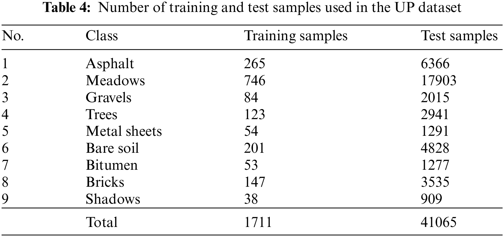
The UP image covers an urban area of University of Pavia, Northern Italy. It was captured by the Reflective Optics System Imaging Spectrometer (ROSIS) sensor on July 08, 2002. This dataset has 115 spectral bands across the spectral range from 0.43 to 0.86 μm where 12 noisy bands were removed. The spatial dimension of this scene is 610 × 340 with spatial resolution of 1.3 m/pixel. Fig. 9 shows the false color image of UP dataset and the corresponding ground truth image.

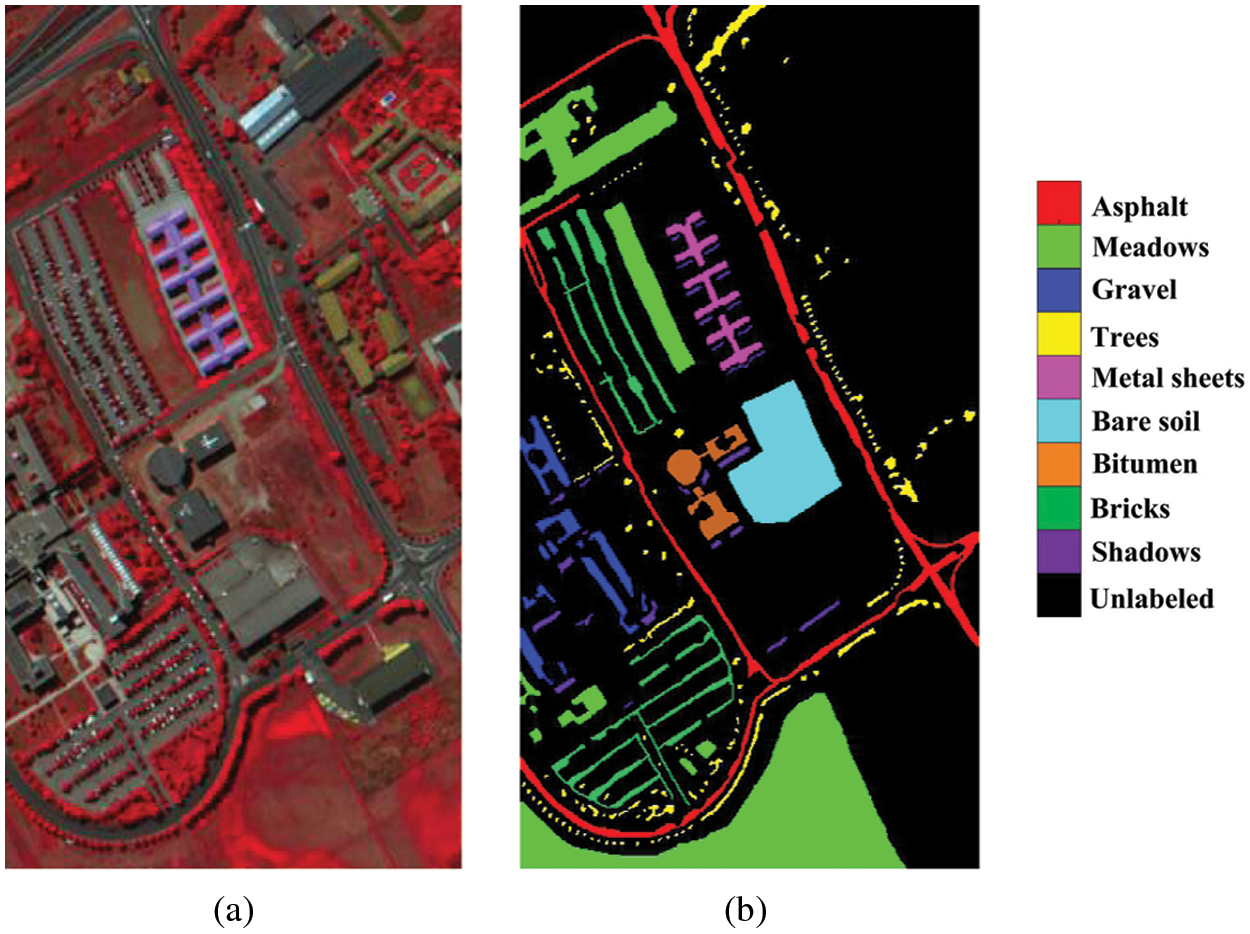
Figure 9: UP dataset. (a) False color image. (b) Ground truth

The SA dataset was also recorded by the AVIRIS sensor over the area of Salinas Valley, California, USA with a spectral range from 0.36 to 2.5 μm. It contains 224 spectral bands and has a size of 512 × 217 with spatial resolution of 3.7 m/pixel. For classification purpose, 16 classes were defined for this image. Before the experiments, 20 bands were removed due to the water absorption and noise. Fig. 10 shows the false color image of SA dataset and the corresponding ground truth image.

Figure 10: SA dataset. (a) False color image. (b) Ground truth

5.2 Experimental Design

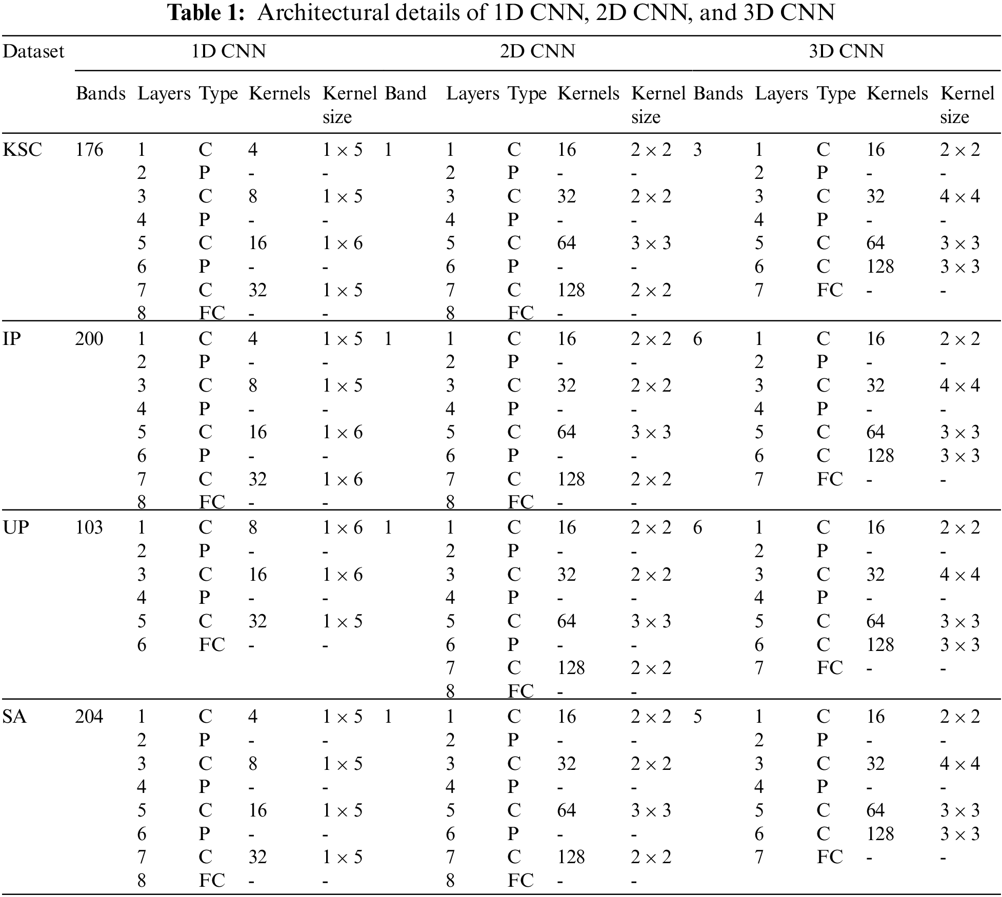
In our experiments, we have empirically selected the parameters for 1D CNN, 2D CNN, and 3D CNN. Table 1 shows the parameter setting of the models on KSC, IP, UP, and SA datasets, where C, P, and FC are representing the convolutional, pooling, and fully connected layers, respectively. For the convolutional layer, kernel size is varied according to the datasets. In case of pooling layer, max pooling [99] has been selected with pool size of 2. The learning rate was set as 0.01 with the weight decay of 1e−6. The experiments were conducted for 200 epochs with mini batch size of 100. For fairness, we have used 20 trials for each method, where each trial contains different distribution of training and test samples. The experiments were performed using laptop with Intel Core(TM) i5-6200U 2.4-GHz CPU with 8 GB memory and an NVIDIA GeForce 940 M GPU. All the experiments were implemented using Keras 2.2.4 and Tensorow 1.12.0 (backend library).

To measure the quantitative results, we have adopted three popular indexes: overall accuracy (OA), average accuracy (AA), and kappa coefficient (Kp). The OA refers the total number of accurately classified test samples over entire test samples. The AA represents the average of class-wise accuracies. The Kp measures the similarity among classification map and ground truth map. In addition, standard deviation has been reported for each index.

5.3 Sensitivity to the Number of Bands in 3D CNN

Previous studies have reported that selection of number of spectral bands are highly responsible for affecting the performance of HSI classification. On the one hand, considering too few bands may cause unsatisfactory performance due to the limited amount of spectral information. On the other hand, excessive bands may reduce the classification accuracy and increase the computational cost [80]. To address this issue, an empirical band analysis has been conducted using PCA on 3D CNN to select the optimal number of bands. In Fig. 11, we can observe that OA gets decreased after third band for KSC dataset with increasing computation time. Therefore, we have considered only three bands for KSC dataset. Similar observations have been found from the remaining datasets. For example, the OA gets saturated or starts decreasing after 6th, 6th, and 5th bands for IP, UP, and SA dataset, respectively. Hence, the number of bands has been set as 6, 6 and 5 for IP, UP, and SA dataset, respectively.

Figure 11: Sensitivity to the number of bands on 3D CNN for KSC, IP, UP, and SA datasets. (a) OA vs. number of bands. (b) Training time vs. number of bands

5.4 Sensitivity to the Number of Training Sample

As HSI contains limited labeled samples, selection of number of training samples is an important criterion for HSI classification. Therefore, we have presented an analysis to select the number of training samples for all the considered datasets and models. For KSC and IP datasets, the analysis have been performed by randomly selecting 4%, 6%, 8%, 10%, and 12% training samples from each class. Compared with KSC and IP datasets, UP and SA datasets contain huge number of training samples. Therefore, the proportion of training samples were considered as 1%, 2%, 3%, 4%, 5% for UP dataset and 1%, 1.5%, 2%, 2.5%, 3% for SA dataset. As shown in Fig. 12, the OA gets improved when number of training samples are increased. The OA of FFCNN reaches above 99% and 98% for KSC and IP dataset, respectively when 10% training samples were considered. Beside this, we have achieved marginal improvement in OA with increasing computation time when more than 10% training samples were considered. Therefore, we have found 10% training samples to be an optimal choice for KSC and IP datasets. Similarly, 4% and 2.5% training samples have been found to be suitable for UP and SA datasets, respectively.

Figure 12: Sensitivity to the number of training samples using 1D CNN, 2D CNN, 3D CNN, and FFCNN. (a) KSC. (b) IP. (c) UP. (d) SA

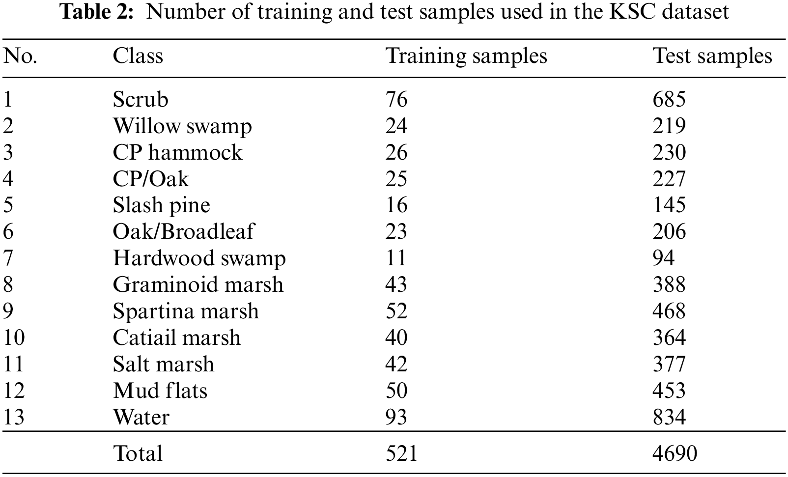
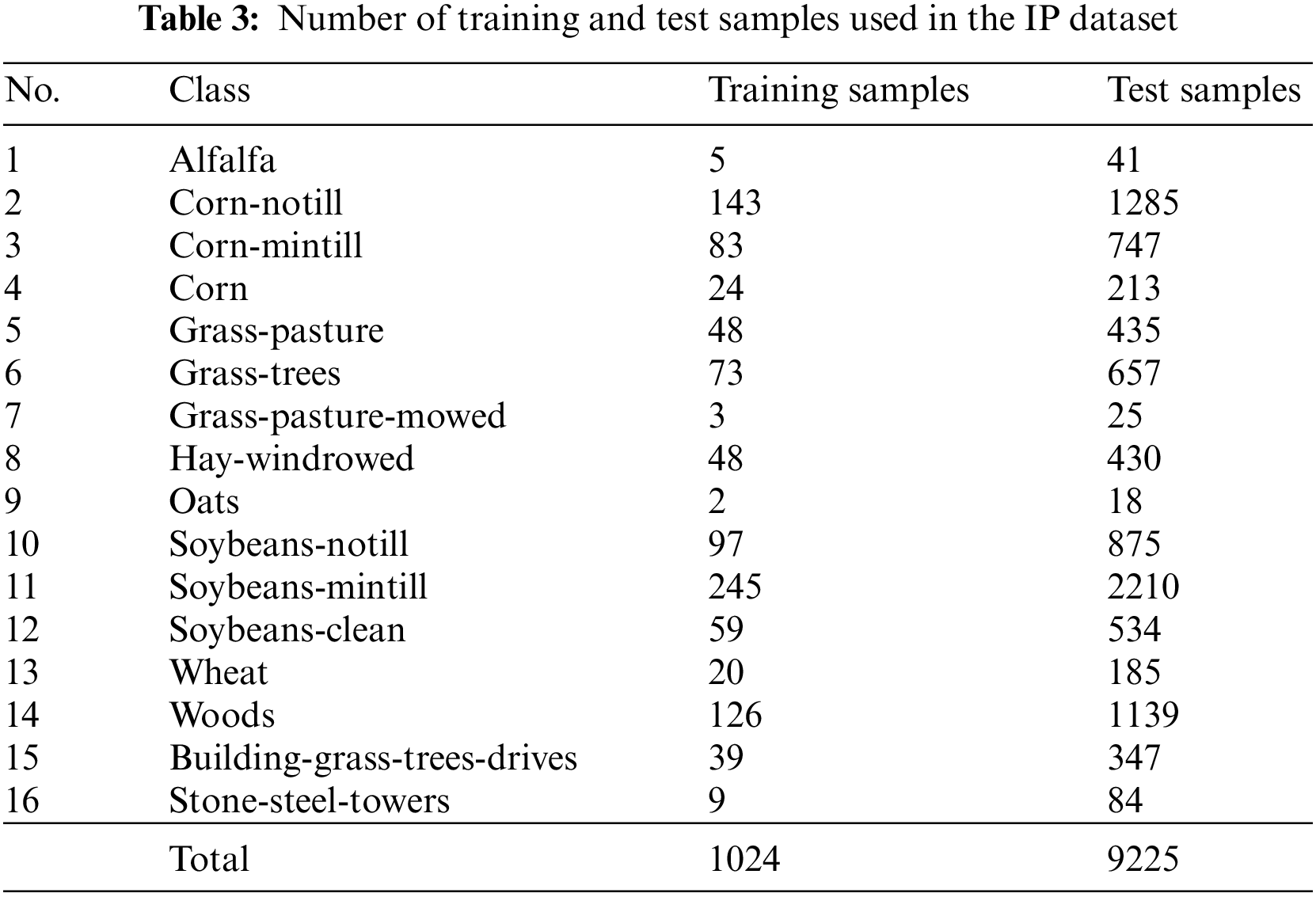
Based on the above analysis, we have randomly selected 10% training samples from each class of KSC and IP datasets and remaining samples were used as test samples. The detailed distribution of training and test samples of KSC and IP datasets are listed in Tables 2 and 3, respectively. For UP and SA datasets, 4% and 2.5% training samples were randomly selected from each class respectively and rest samples were used as test samples. The detailed distribution of training and test samples of UP and SA datasets have been reported in Tables 4 and 5, respectively.

5.5 Classification Results

5.5.1 Classification Results on KSC

The classification results of four CNN based methods on KSC dataset have been shown in Table 6. The first 13 rows of the table indicate class-wise accuracies, and the remaining three rows present statistical results in terms of OA, AA, and Kp. It has been observed that the performance of 2D CNN is better than 1D CNN because spatial information has more impact than spectral information. Further, compared with 2D CNN, 3D CNN and FFCNN has achieved better classification results due to the presence of both spectral and spatial information. Lastly, when we compared the results of 3D CNN vs. FFCNN, we found that FFCNN performed better due to the consideration of feature fusion. It is worth mentioning that FFCNN has achieved almost accurate classification accuracy for eight classes (including Scrub, CP Hammock, Hardwood swamp, Graminoid marsh, Spartina marsh, Catiail marsh, Salt marsh, Mud flats) and obtained perfect classification for Water class. For all the classes, FFCNN has achieved more than 94% classification accuracy. Among four methods, the statistical performance of FFCNN is found to be better in terms of OA, AA, and Kp.

Along with the statistical results, a classification map has been presented for all four datasets using all considered models. The classification map on the KSC dataset is shown in Fig. 13. It can be observed that 1D CNN and 2D CNN misclassify many samples whereas the classification maps of 3D CNN and FFCNN are better than 1D CNN and 2D CNN due to the effect of spectral and spatial information. As the number of labeled samples in KSC is very less, therefore it is very difficult to visually differentiate the classification maps of 3D CNN and FFCNN.

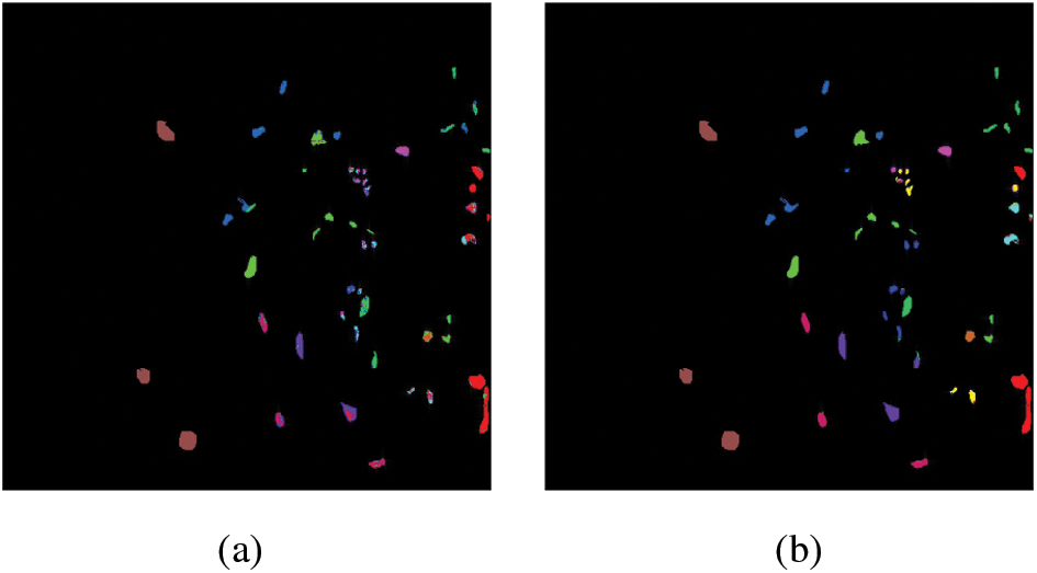
Figure 13: Classification maps for KSC dataset. (a) 1D CNN. (b) 2D CNN. (c) 3D CNN. (d) FFCNN

5.5.2 Classification Results on IP

The classification results on IP dataset have been summarized in Table 7. It has been observed that 1D CNN obtained below 70% classification accuracy in many classes. The performance of other methods is far better than 1D CNN. For 2D CNN, each class has achieved over 84% classification accuracy. In case of 3D CNN and FFCNN, all the classes have obtained more than 91% classification accuracy. For the Oats class, the classification results of 1D CNN and 2D CNN are not satisfactory. Compared with these two methods, the performance of 3D CNN has increased by 61.11% and 13.89%, respectively whereas the performance of FFCNN has improved by 60.83% and 13.61%, respectively. Compared with 3D CNN, FFCNN has obtained better classification accuracy in many classes and achieved higher statistical results in terms of OA, AA, and Kp.

The classification maps of four methods on IP dataset are shown in Fig. 14. Due to the absence of spatial information, 1D CNN suffers from misclassification of objects. Similarly, 2D CNN fails to produce smooth classification maps due to the lack of spectral information. Besides this, 3D CNN and FFCNN have taken advantage of both spectral-spatial information and yielded better classification maps. Compared with 3D CNN, FFCNN has achieved better clarity on Soybeans-mintill class.

Figure 14: Classification maps for IP dataset. (a) 1D CNN. (b) 2D CNN. (c) 3D CNN. (d) FFCNN

5.5.3 Classification Results on UP

The classification results of four methods on UP datasets have been depicted in Table 8. It can be observed that Gravel, Bare soil, and Bitumen were the most difficult class to be classified by the 1D CNN. However, other methods have achieved more than 92% classification accuracy in most of the classes. Therefore, their statistical performance is far better than 1D CNN. The performance of 3D CNN and FFCNN are superior to 1D CNN and 2D CNN in every respect. Compared with 3D CNN, FFCNN obtains better classification results because of its fusion technique. It is worth noting that FFCNN has achieved almost correct classification results for Asphalt, Meadows, Metal Sheets, and Bare soil. Moreover, compared among four methods, FFCNN has best classification accuracies in term of OA, AA, and Kp.

The classification maps of four methods on UP dataset are shown in Fig. 15. Many samples belonging to the Bare soil class are misclassified by 1D CNN due to similar spectral characteristics and lack of spatial information. However, other methods have shown finer regional clarity in the bare soil class. Moreover, FFCNN has gained improved boundary appearance in the Bitumen class.

Figure 15: Classification maps for UP dataset. (a) 1D CNN. (b) 2D CNN. (c) 3D CNN. (d) FFCNN

5.5.4 Classification Results on SA

The classification results of four CNN based methods on SA datasets have been reported in Table 9. It can be observed that all the considered methods have obtained more than 96% classification accuracy in most of the classes. However, the performance of 1D CNN is not adequate specifically for Vinyard_untrained class. Compared with this method, the performances of 2D CNN, 3D CNN, and FFCNN have increased by 41.91%, 44.8%, and 47.53%, respectively. Further, compared with 2D CNN, 3D CNN and FFCNN have achieved better classification results. Among four methods, FFCNN has achieved the best classification accuracies in most of the classes. After FFCNN, 3D CNN has achieved the highest classification accuracy in terms of OA, AA, and Kp. Thus, 3D CNN is the closest competitor of FFCNN.

The classification maps of four methods on SA dataset are shown in Fig. 16. It can be observed that 1D CNN, 2D CNN, and 3D CNN have misclassified many samples in Grapes_untrained and Vinyard_untrained classes, which make noisy classification maps. However, FFCNN successfully classified all the classes and was able to generate a smooth classification map. Moreover, compared with 3D CNN, FFCNN has obtained finer uniformity in Brocoli_green_weeds_1 and Celery classes.

Figure 16: Classification maps for UP dataset. (a) 1D CNN. (b) 2D CNN. (c) 3D CNN. (d) FFCNN

5.6 Analysis on Computational Time

In this section, we have discussed the computational time of four CNN based HSI classification methods. The training time (for 200 epochs) and test time on all the considered datasets are reported in Table 10. The training time of 1D CNN is very less due to the structure of 1D pixel vector. The 2D CNN is faster on training time than 3D CNN and FFCNN due to the consideration of single band. On the other hand, 3D CNN and FFCNN cost more training time because of the increasing parameters of the 3D convolution operations.

During testing, the computation time of 1D CNN and 2D CNN were less as compared to 3D CNN and FFCNN. This is because 1D CNN and 2D CNN has less number of parameters whereas 3D CNN and FFCNN involves complex 3D convolution operations. Lastly, while comparing 3D CNN and FFCNN, FFCNN consumes little bit more time due to the usage of feature fusion technique.

6  Conclusion and Future Guidelines

Recently, deep learning models have drawn a significant amount of attention for HSI classification. Among various deep learning models, CNN has shown effectiveness in feature extraction and demonstrated state-of-the-art performance in HSI classification. Therefore, in this paper, we have presented a systematic review on the literature of HSI classification, which is based on various CNN architectures. Further, experimental analysis on four well-known HSI datasets has been presented with four CNN based models namely 1D CNN, 2D CNN, 3D CNN, and FFCNN. In addition, we have shown the effect of the selection of a number of bands and a number of training samples. The experimental results demonstrated that the performance was not good enough when only spectral information or spatial information was used. But, classification accuracy had increased significantly when both spectral and spatial information were considered. The accuracy had further improved when the feature fusion technique was applied. For this reason, we have found that the overall performance of FFCNN is better than other methods for all considered datasets. Moreover, 3D CNN has shown satisfactory classification results and thus, it is the closest competitor of FFCNN. In the context of CNN based HSI classification, we believe that the following are the challenges and future guidelines that might be useful in future research.

(1)   To exploit the spectral information, 1D CNN may be a suitable choice because it has a simple internal structure and can be easily implemented. In addition, it takes less time to process the pixel vectors of HSI datasets. However, 1D CNN alone is unable to produce satisfactory performance.

(2)   The 2D CNN is able to efficiently exploit the spatial information of HSI and significantly improves the classification performance. However, 2D CNN alone cannot find the subtle differences among small objects due to the insufficient spectral information. Therefore, 2D CNN can be integrated with 1D CNN to enhance the classification performance.

(3)   3D CNN provides a way to extract join spectral-spatial feature extraction. Nevertheless, joint spectral-spatial feature extraction leads to information loss [80,88] and hence we believe that separate spectral and spatial feature extraction should be adopted to achieve better classification performance.

(4)   Recently, the feature fusion technique has delivered superior performance in HSI classification. However, the system’s performance varies depending on how the fusion of features has been done. For example, there are two types of feature fusion techniques proposed in literature: early fusion and late fusion. The early fusion and late fusion are developed based on the feature level and decision score level, respectively [140]. Both fusion techniques have their own advantages and disadvantages. Hence, there are many scopes to improve the HSI classification performance by analyzing the different ways of feature fusion.

(5)   HSI has a huge number of bands, and hence, the use of 2D CNN and 3D CNN demand for a selection of a few informative bands to reduce the computational cost and redundant information. More number of bands leads to an increase in computational cost while fewer bands can be responsible for information loss. Therefore, an optimum number of band selection is a critical challenge in the HSI classification system and requires attention.

(6)   Another challenge in HSI classification is the limited availability of training samples. Researchers are trying to design a system that can achieve high classification accuracy by utilizing as few training samples as possible. Still, it is a challenging task as insufficient training samples create an overfitting problem.

Funding Statement: The authors received no specific funding for this study.

Conflicts of Interest: The authors declare that they have no conflicts of interest to report regarding the present study.

References

1. Chen, Y., Lin, Z., Zhao, X., Wang, G., & Gu, Y. (2014). Deep learning-based classification of hyperspectral data. IEEE Journal of Selected Topics in Applied Earth Observations and Remote Sensing, 7(6), 2094-2107. [Google Scholar] [CrossRef]
2. van der Meer, F. (2004). Analysis of spectral absorption features in hyperspectral imagery. International Journal of Applied Earth Observation and Geoinformation, 5(1), 55-68. [Google Scholar] [CrossRef]
3. Yuen, P. W., & Richardson, M. (2010). An introduction to hyperspectral imaging and its application for security, surveillance and target acquisition. The Imaging Science Journal, 58(5), 241-253. [Google Scholar] [CrossRef]
4. Egerton, R. F. (2011). Electron Energy-Loss Spectroscopy in the Electron Microscope. New York, London: Springer Science & Business Media.
5. Hege, E. K., O’Connell, D., Johnson, W., Basty, S., Dereniak, E. L. (2004). Hyperspectral imaging for astronomy and space surveillance. In: Imaging spectrometry IX, vol. 5159. International Society for Optics and Photonics.
6. Gowen, A. A., O’Donnell, C. P., Cullen, P. J., Downey, G., & Frias, J. M. (2007). Hyperspectral imaging–An emerging process analytical tool for food quality and safety control. Trends in Food Science & Technology, 18(12), 590-598. [Google Scholar] [CrossRef]
7. Makki, I., Younes, R., Francis, C., Bianchi, T., & Zucchetti, M. (2017). A survey of landmine detection using hyperspectral imaging. ISPRS Journal of Photogrammetry and Remote Sensing, 124, 40-53. [Google Scholar] [CrossRef]
8. Lacar, F., Lewis, M., Grierson, I. (2001). Use of hyperspectral imagery for mapping grape varieties in the barossa valley, South Australia. In: Scanning the present and resolving the future. Proceedings of IEEE 2001 International Geoscience and Remote Sensing Symposium (Cat. No. 01CH37217), vol. 6. Sydney, NSW, Australia, IEEE.
9. Metternicht, G., & Zinck, J. (2003). Remote sensing of soil salinity: Potentials and constraints. Remote Sensing of Environment, 85(1), 1-20. [Google Scholar] [CrossRef]
10. Wang, Y., & Duan, H. (2018). Classification of hyperspectral images by SVM using a composite kernel by employing spectral, spatial and hierarchical structure information. Remote Sensing, 10(3), 441. [Google Scholar] [CrossRef]
11. Tarabalka, Y., Fauvel, M., Chanussot, J., & Benediktsson, J. A. (2010). SVM-and MRF-based method for accurate classification of hyperspectral images. IEEE Geoscience and Remote Sensing Letters, 7(4), 736-740. [Google Scholar] [CrossRef]
12. Liu, J., Zhou, X., Huang, J., Liu, S., & Li, H. (2017). Semantic classification for hyperspectral image by integrating distance measurement and relevance vector machine. Multimedia Systems, 23(1), 95-104. [Google Scholar] [CrossRef]
13. Li, W., Tramel, E. W., Prasad, S., & Fowler, J. E. (2013). Nearest regularized subspace for hyperspectral classification. IEEE Transactions on Geoscience and Remote Sensing, 52(1), 477-489. [Google Scholar] [CrossRef]
14. Huang, K., Li, S., Kang, X., & Fang, L. (2016). Spectral–spatial hyperspectral image classification based on KNN. Sensing and Imaging, 17(1), 1. [Google Scholar] [CrossRef]
15. Ma, L., Crawford, M. M., & Tian, J. (2010). Local manifold learning-based -nearest-neighbor for hyperspectral image classification. IEEE Transactions on Geoscience and Remote Sensing, 48(11), 4099-4109. [Google Scholar] [CrossRef]
16. Peng, J., Li, L., & Tang, Y. Y. (2018). Maximum likelihood estimation-based joint sparse representation for the classification of hyperspectral remote sensing images. IEEE Transactions on Neural Networks and Learning Systems, 30(6), 1790-1802. [Google Scholar] [CrossRef]
17. Richards, J. A., & Jia, X. (2008). Using suitable neighbors to augment the training set in hyperspectral maximum likelihood classification. IEEE Geoscience and Remote Sensing Letters, 5(4), 774-777. [Google Scholar] [CrossRef]
18. Bajpai, S., Singh, H. V., Kidwai, N. R. (2017). Feature extraction & classification of hyperspectral images using singular spectrum analysis & multinomial logistic regression classifiers. 2017 International Conference on Multimedia, Signal Processing and Communication Technologies (IMPACT), IEEE, Aligarh, India.
19. Li, J., Bioucas-Dias, J. M., & Plaza, A. (2012). Semisupervised hyperspectral image classification using soft sparse multinomial logistic regression. IEEE Geoscience and Remote Sensing Letters, 10(2), 318-322. [Google Scholar] [CrossRef]
20. Zhu, C., & Yang, X. (1998). Study of remote sensing image texture analysis and classification using wavelet. International Journal of Remote Sensing, 19(16), 3197-3203. [Google Scholar] [CrossRef]
21. Pesaresi, M., Gerhardinger, A., & Kayitakire, F. (2008). A robust built-up area presence index by anisotropic rotation-invariant textural measure. IEEE Journal of Selected Topics in Applied Earth Observations and Remote Sensing, 1(3), 180-192. [Google Scholar] [CrossRef]
22. Pesaresi, M., & Benediktsson, J. A. (2001). A new approach for the morphological segmentation of high-resolution satellite imagery. IEEE Transactions on Geoscience and Remote Sensing, 39(2), 309-320. [Google Scholar] [CrossRef]
23. Li, W., & Du, Q. (2014). Gabor-filtering-based nearest regularized subspace for hyperspectral image classification. IEEE Journal of Selected Topics in Applied Earth Observations and Remote Sensing, 7(4), 1012-1022. [Google Scholar] [CrossRef]
24. Khan, M. A., Muhammad, K., Sharif, M., Akram, T., Kadry, S. (2021). Intelligent fusion-assisted skin lesion localization and classification for smart healthcare. Neural Computing and Applications, 1–16. DOI 10.1007/s00521-021-06490-w. [CrossRef]
25. Khan, S., Khan, M. A., Alhaisoni, M., Tariq, U., & Yong, H.-S. (2021). Human action recognition: A paradigm of best deep learning features selection and serial based extended fusion. Sensors, 21(23), 7941. [Google Scholar] [CrossRef]
26. LeCun, Y., Bengio, Y., & Hinton, G. (2015). Deep learning. Nature, 521(7553), 436-444. [Google Scholar] [CrossRef]
27. Schmidhuber, J. (2015). Deep learning in neural networks: An overview. Neural Networks, 61, 85-117. [Google Scholar] [CrossRef]
28. Deng, L., & Yu, D. (2014). Deep learning: Methods and applications. Foundations and Trends in Signal Processing, 7(3–4), 197-387. [Google Scholar] [CrossRef]
29. Bengio, Y., Goodfellow, I., Courville, A. (2017). Deep learning, vol. 1. Cambridge, MA, USA: MIT Press.
30. Sundararajan, K., Garg, L., Srinivasan, K., Bashir, A. K., & Kaliappan, J. (2021). A contemporary review on drought modeling using machine learning approaches. Computer Modeling in Engineering & Sciences, 128(2), 447-487. [Google Scholar] [CrossRef]
31. Cheng, R., Yin, X. M., & Chen, L. (2022). Machine learning enhanced boundary element method: Prediction of Gaussian quadrature points. Computer Modeling in Engineering & Sciences, 131(1), 445-464. [Google Scholar] [CrossRef]
32. Ioannidou, A., Chatzilari, E., Nikolopoulos, S., & Kompatsiaris, I. (2017). Deep learning advances in computer vision with 3D data: A survey. ACM Computing Surveys, 50(2), 1-38. [Google Scholar] [CrossRef]
33. Szegedy, C., Toshev, A., Erhan, D. (2013). Deep neural networks for object detection. In: Advances in neural information processing systems. Harrahs and Harveys, Lake Tahoe, USA.
34. Jadhav, A. R., Ghontale, A. G., Shrivastava, V. K. (2019). Segmentation and border detection of melanoma lesions using convolutional neural network and SVM. Computational Intelligence: Theories, Applications and Future Directions, vol. I, pp. 97–108. Singapore: Springer.
35. Pattnaik, G., Shrivastava, V. K., & Parvathi, K. (2020). Transfer learning-based framework for classification of pest in tomato plants. Applied Artificial Intelligence, 34(13), 981-993. [Google Scholar] [CrossRef]
36. Collobert, R., Weston, J., Bottou, L., Karlen, M., & Kavukcuoglu, K. (2011). Natural language processing (almost) from scratch. Journal of Machine Learning Research, 12, 2493-2537. [Google Scholar]
37. Dessì, D., Osborne, F., Recupero, D. R., Buscaldi, D., & Motta, E. (2021). Generating knowledge graphs by employing natural language processing and machine learning techniques within the scholarly domain. Future Generation Computer Systems, 116, 253-264. [Google Scholar] [CrossRef]
38. Signoroni, A., Savardi, M., Baronio, A., & Benini, S. (2019). Deep learning meets hyperspectral image analysis: A multidisciplinary review. Journal of Imaging, 5(5), 52. [Google Scholar] [CrossRef]
39. Abdi, G., Samadzadegan, F., & Reinartz, P. (2017). Spectral–spatial feature learning for hyperspectral imagery classification using deep stacked sparse autoencoder. Journal of Applied Remote Sensing, 11(4), 042604. [Google Scholar] [CrossRef]
40. Menezes, J., & Poojary, N. (2021). Hyperspectral image data classification with refined spectral spatial features based on stacked autoencoder approach. Recent Patents on Engineering, 15(2), 140-149. [Google Scholar] [CrossRef]
41. Le Roux, N., & Bengio, Y. (2010). Deep belief networks are compact universal approximators. Neural Computation, 22(8), 2192-2207. [Google Scholar] [CrossRef]
42. Chintada, K. R., Yalla, S. P., Uriti, A. (2021). A deep belief network based land cover classification. 2021 Innovations in Power and Advanced Computing Technologies (i-PACT). University of Malaya, Kuala Lumpur, Malaysia.
43. Krizhevsky, A., Sutskever, I., Hinton, G. E. (2012). Imagenet classification with deep convolutional neural networks. Advances in neural information processing systems, vol. 25. Harrahs and Harveys, Lake Tahoe, USA.
44. Patel, H., & Upla, K. P. (2021). A shallow network for hyperspectral image classification using an autoencoder with convolutional neural network. Multimedia Tools and Applications, 81, 1-20. [Google Scholar] [CrossRef]
45. Yu, S., Jia, S., & Xu, C. (2017). Convolutional neural networks for hyperspectral image classification. Neurocomputing, 219, 88-98. [Google Scholar] [CrossRef]
46. Ortac, G., & Ozcan, G. (2021). Comparative study of hyperspectral image classification by multidimensional convolutional neural network approaches to improve accuracy. Expert Systems with Applications, 182, 115280. [Google Scholar] [CrossRef]
47. Li, H. C., Li, S. S., Hu, W. S., Feng, J. H., & Sun, W. W. (2021). Recurrent feedback convolutional neural network for hyperspectral image classification. IEEE Geoscience and Remote Sensing Letters, 19, 1-5. [Google Scholar] [CrossRef]
48. Medus, L. D., Saban, M., Francés-Víllora, J. V., Bataller-Mompeán, M., & Rosado-Muñoz, A. (2021). Hyperspectral image classification using CNN: Application to industrial food packaging. Food Control, 125, 107962. [Google Scholar] [CrossRef]
49. Vaddi, R., & Manoharan, P. (2020). Hyperspectral image classification using CNN with spectral and spatial features integration. Infrared Physics & Technology, 107, 103296. [Google Scholar] [CrossRef]
50. Yan, Y., Yao, X. J., Wang, S. H., & Zhang, Y. D. (2021). A survey of computer-aided tumor diagnosis based on convolutional neural network. Biology, 10(11), 1084. [Google Scholar] [CrossRef]
51. Zhang, Y. D., Satapathy, S. C., Guttery, D. S., Górriz, J. M., & Wang, S. H. (2021). Improved breast cancer classification through combining graph convolutional network and convolutional neural network. Information Processing & Management, 58(2), 102439. [Google Scholar] [CrossRef]
52. Guo, H., Liu, J., Yang, J., Xiao, Z., & Wu, Z. (2020). Deep collaborative attention network for hyperspectral image classification by combining 2-D CNN and 3-D CNN. IEEE Journal of Selected Topics in Applied Earth Observations and Remote Sensing, 13, 4789-4802. [Google Scholar] [CrossRef]
53. Wan, S., Pan, S., Zhong, P., Chang, X., & Yang, J. (2021). Dual interactive graph convolutional networks for hyperspectral image classification. IEEE Transactions on Geoscience and Remote Sensing, 60, [Google Scholar] [CrossRef]
54. Imani, M., & Ghassemian, H. (2020). An overview on spectral and spatial information fusion for hyperspectral image classification: Current trends and challenges. Information Fusion, 59, 59-83. [Google Scholar] [CrossRef]
55. Ge, Z., Cao, G., Li, X., & Fu, P. (2020). Hyperspectral image classification method based on 2D–3D CNN and multibranch feature fusion. IEEE Journal of Selected Topics in Applied Earth Observations and Remote Sensing, 13, 5776-5788. [Google Scholar] [CrossRef]
56. Borzov, S., & Potaturkin, O. (2018). Spectral-spatial methods for hyperspectral image classification. Review. Optoelectronics, Instrumentation and Data Processing, 54(6), 582-599. [Google Scholar] [CrossRef]
57. Jia, S., Jiang, S., Lin, Z., Li, N., & Xu, M. (2021). A survey: Deep learning for hyperspectral image classification with few labeled samples. Neurocomputing, 448, 179-204. [Google Scholar] [CrossRef]
58. Xie, S., Yu, Z., & Lv, Z. (2021). Multi-disease prediction based on deep learning: A survey. Computer Modeling in Engineering & Sciences, 128(2), 489-522. [Google Scholar] [CrossRef]
59. Ma, L., Liu, Y., Zhang, X., Ye, Y., & Yin, G. (2019). Deep learning in remote sensing applications: A meta-analysis and review. ISPRS Journal of Photogrammetry and Remote Sensing, 152, 166-177. [Google Scholar] [CrossRef]
60. Gewali, U. B., Monteiro, S. T., Saber, E. (2018). Machine learning based hyperspectral image analysis: A survey. arXiv preprint arXiv:1802.08701.
61. Khan, M. J., Khan, H. S., Yousaf, A., Khurshid, K., & Abbas, A. (2018). Modern trends in hyperspectral image analysis: A review. IEEE Access, 6, 14118-14129. [Google Scholar] [CrossRef]
62. Ghamisi, P., Plaza, J., Chen, Y., Li, J., & Plaza, A. J. (2017). Advanced spectral classifiers for hyperspectral images: A review. IEEE Geoscience and Remote Sensing Magazine, 5(1), 8-32. [Google Scholar] [CrossRef]
63. He, L., Li, J., Liu, C., & Li, S. (2017). Recent advances on spectral–spatial hyperspectral image classification: An overview and new guidelines. IEEE Transactions on Geoscience and Remote Sensing, 56(3), 1579-1597. [Google Scholar] [CrossRef]
64. Li, S., Song, W., Fang, L., Chen, Y., & Ghamisi, P. (2019). Deep learning for hyperspectral image classification: An overview. IEEE Transactions on Geoscience and Remote Sensing, 57(9), 6690-6709. [Google Scholar] [CrossRef]
65. Kruger, N., Janssen, P., Kalkan, S., Lappe, M., & Leonardis, A. (2012). Deep hierarchies in the primate visual cortex: What can we learn for computer vision?. IEEE Transactions on Pattern Analysis and Machine Intelligence, 35(8), 1847-1871. [Google Scholar] [CrossRef]
66. Yue, J., Zhao, W., Mao, S., & Liu, H. (2015). Spectral–spatial classification of hyperspectral images using deep convolutional neural networks. Remote Sensing Letters, 6(6), 468-477. [Google Scholar] [CrossRef]
67. He, M., Li, B., Chen, H. (2017). Multi-scale 3D deep convolutional neural network for hyperspectral image classification. 2017 IEEE International Conference on Image Processing (ICIP), IEEE. Beijing, China.
68. Zhang, H., Li, Y., Zhang, Y., & Shen, Q. (2017). Spectral-spatial classification of hyperspectral imagery using a dual-channel convolutional neural network. Remote Sensing Letters, 8(5), 438-447. [Google Scholar] [CrossRef]
69. Li, Y., Zhang, H., & Shen, Q. (2017). Spectral–spatial classification of hyperspectral imagery with 3D convolutional neural network. Remote Sensing, 9(1), 67. [Google Scholar] [CrossRef]
70. Cao, X., Yao, J., Xu, Z., & Meng, D. (2020). Hyperspectral image classification with convolutional neural network and active learning. IEEE Transactions on Geoscience and Remote Sensing, 58(7), 4604--4616. [Google Scholar] [CrossRef]
71. Kutluk, S., Kayabol, K., & Akan, A. (2021). A new CNN training approach with application to hyperspectral image classification. Digital Signal Processing, 113, 103016. [Google Scholar] [CrossRef]
72. Li, Y., Xie, W., & Li, H. (2017). Hyperspectral image reconstruction by deep convolutional neural network for classification. Pattern Recognition, 63, 371-383. [Google Scholar] [CrossRef]
73. Chang, Y., Yan, L., Fang, H., Zhong, S., & Liao, W. (2018). HSI-DeNet: Hyperspectral image restoration via convolutional neural network. IEEE Transactions on Geoscience and Remote Sensing, 57(2), 667-682. [Google Scholar] [CrossRef]
74. Yuan, Q., Zhang, Q., Li, J., Shen, H., & Zhang, L. (2018). Hyperspectral image denoising employing a spatial–spectral deep residual convolutional neural network. IEEE Transactions on Geoscience and Remote Sensing, 57(2), 1205-1218. [Google Scholar] [CrossRef]
75. Liu, B., Yu, X., Zhang, P., Tan, X., & Yu, A. (2017). A semi-supervised convolutional neural network for hyperspectral image classification. Remote Sensing Letters, 8(9), 839-848. [Google Scholar] [CrossRef]
76. Hu, W., Huang, Y., Wei, L., Zhang, F., & Li, H. (2015). Deep convolutional neural networks for hyperspectral image classification. Journal of Sensors, 2015, [Google Scholar] [CrossRef]
77. Wu, H., & Prasad, S. (2017). Convolutional recurrent neural networks forhyperspectral data classification. Remote Sensing, 9(3), 298. [Google Scholar] [CrossRef]
78. Yang, X., Ye, Y., Li, X., Lau, R. Y., & Zhang, X. (2018). Hyperspectral image classification with deep learning models. IEEE Transactions on Geoscience and Remote Sensing, 56(9), 5408-5423. [Google Scholar] [CrossRef]
79. Chen, Y., Zhu, K., Zhu, L., He, X., & Ghamisi, P. (2019). Automatic design of convolutional neural network for hyperspectral image classification. IEEE Transactions on Geoscience and Remote Sensing, 57(9), 7048-7066. [Google Scholar] [CrossRef]
80. Chen, Y., Jiang, H., Li, C., Jia, X., & Ghamisi, P. (2016). Deep feature extraction and classification of hyperspectral images based on convolutional neural networks. IEEE Transactions on Geoscience and Remote Sensing, 54(10), 6232-6251. [Google Scholar] [CrossRef]
81. Sun, G., Zhang, X., Jia, X., Ren, J., & Zhang, A. (2020). Deep fusion of localized spectral features and multi-scale spatial features for effective classification of hyperspectral images. International Journal of Applied Earth Observation and Geoinformation, 91, 102157. [Google Scholar] [CrossRef]
82. Shrivastava, V. K., Pradhan, M. K., Minz, S., & Thakur, M. P. (2019). Rice plant disease classification using transfer learning of deep convolution neural network. International Archives of the Photogrammetry, Remote Sensing & Spatial Information Sciences, 42(3), [Google Scholar] [CrossRef]
83. Shrivastava, V. K., Pradhan, M. K., Thakur, M. P. (2021). Application of pre-trained deep convolutional neural networks for rice plant disease classification. 2021 International Conference on Artificial Intelligence and Smart Systems (ICAIS), IEEE. JCT College of Engineering and Technology, Pichanur, Tamil Nadu.
84. Simonyan, K., Zisserman, A. (2014). Very deep convolutional networks for large-scale image recognition. arXiv preprint arXiv:1409.1556.
85. Zhang, M., Li, W., & Du, Q. (2018). Diverse region-based CNN for hyperspectral image classification. IEEE Transactions on Image Processing, 27(6), 2623-2634. [Google Scholar] [CrossRef]
86. Cao, X., Zhou, F., Xu, L., Meng, D., & Xu, Z. (2018). Hyperspectral image classification with Markov random fields and a convolutional neural network. IEEE Transactions on Image Processing, 27(5), 2354-2367. [Google Scholar] [CrossRef]
87. Shi, C., & Wang, L. (2014). Incorporating spatial information in spectral unmixing: A review. Remote Sensing of Environment, 149, 70-87. [Google Scholar] [CrossRef]
88. Xu, Y., Zhang, L., Du, B., & Zhang, F. (2018). Spectral–spatial unified networks for hyperspectral image classification. IEEE Transactions on Geoscience and Remote Sensing, 56(10), 5893-5909. [Google Scholar] [CrossRef]
89. Vaddi, R., Manoharan, P. (2018). Probabilistic PCA based hyper spectral image classification for remote sensing applications. International Conference on Intelligent Systems Design and Applications, Springer. Vellore, India.
90. Haque, M. R., Mishu, S. Z. (2019). Spectral-spatial feature extraction using PCA and multi-scale deep convolutional neural network for hyperspectral image classification. 2019 22nd International Conference on Computer and Information Technology (ICCIT), IEEE. Southeast University, Tejgaon, Dhaka, Bangladesh.
91. Xu, X., Li, W., Ran, Q., Du, Q., & Gao, L. (2017). Multisource remote sensing data classification based on convolutional neural network. IEEE Transactions on Geoscience and Remote Sensing, 56(2), 937-949. [Google Scholar] [CrossRef]
92. Jiao, L., Liang, M., Chen, H., Yang, S., & Liu, H. (2017). Deep fully convolutional network-based spatial distribution prediction for hyperspectral image classification. IEEE Transactions on Geoscience and Remote Sensing, 55(10), 5585-5599. [Google Scholar] [CrossRef]
93. Szegedy, C., Liu, W., Jia, Y., Sermanet, P., Reed, S. et al. (2015). Going deeper with convolutions. Proceedings of the IEEE Conference on Computer Vision and Pattern Recognition, Boston, MA, USA.
94. He, K., Zhang, X., Ren, S., Sun, J. (2016). Deep residual learning for image recognition. Proceedings of the IEEE Conference on Computer Vision and Pattern Recognition, Las Vegas, NV, USA.
95. Cheng, G., Li, Z., Han, J., Yao, X., & Guo, L. (2018). Exploring hierarchical convolutional features for hyperspectral image classification. IEEE Transactions on Geoscience and Remote Sensing, 56(11), 6712-6722. [Google Scholar] [CrossRef]
96. Yang, J., Zhao, Y., Chan, J. C. -W., Yi, C. (2016). Hyperspectral image classification using two-channel deep convolutional neural network. 2016 IEEE International Geoscience and Remote Sensing Symposium (IGARSS), IEEE, Beijing, China.
97. Makantasis, K., Karantzalos, K., Doulamis, A., Doulamis, N. (2015). Deep supervised learning for hyperspectral data classification through convolutional neural networks. 2015 IEEE International Geoscience and Remote Sensing Symposium (IGARSS), IEEE, Milan, Italy.
98. Liang, H., & Li, Q. (2016). Hyperspectral imagery classification using sparse representations of convolutional neural network features. Remote Sensing, 8(2), 99. [Google Scholar] [CrossRef]
99. Bera, S., & Shrivastava, V. K. (2020). Effect of pooling strategy on convolutional neural network for classification of hyperspectral remote sensing images. IET Image Processing, 14(3), 480-486. [Google Scholar] [CrossRef]
100. Bera, S., & Shrivastava, V. K. (2020). Analysis of various optimizers on deep convolutional neural network model in the application of hyperspectral remote sensing image classification. International Journal of Remote Sensing, 41(7), 2664-2683. [Google Scholar] [CrossRef]
101. Acquarelli, J., Marchiori, E., Buydens, L., Tran, T., & van Laarhoven, T. (2018). Spectral-spatial classification of hyperspectral images: Three tricks and a new learning setting. Remote Sensing, 10(7), 1156. [Google Scholar] [CrossRef]
102. Chan, R. H., Kan, K. K., Nikolova, M., & Plemmons, R. J. (2020). A two-stage method for spectral–spatial classification of hyperspectral images. Journal of Mathematical Imaging and Vision, 62(6), 790-807. [Google Scholar] [CrossRef]
103. Benediktsson, J. A., Ghamisi, P. (2015). Spectral-spatial classification of hyperspectral remote sensing images. London, UK: Artech House.
104. He, N., Paoletti, M. E., Haut, J. M., Fang, L., & Li, S. (2018). Feature extraction with multiscale covariance maps for hyperspectral image classification. IEEE Transactions on Geoscience and Remote Sensing, 57(2), 755-769. [Google Scholar] [CrossRef]
105. Gao, H., Yang, Y., Li, C., Zhang, X., & Zhao, J. (2019). Convolutional neural network for spectral–spatial classification of hyperspectral images. Neural Computing and Applications, 31(12), 8997-9012. [Google Scholar] [CrossRef]
106. Paoletti, M., Haut, J., Plaza, J., & Plaza, A. (2018). A new deep convolutional neural network for fast hyperspectral image classification. ISPRS Journal of Photogrammetry and Remote Sensing, 145, 120-147. [Google Scholar] [CrossRef]
107. Ding, C., Li, Y., Xia, Y., Wei, W., & Zhang, L. (2017). Convolutional neural networks based hyperspectral image classification method with adaptive kernels. Remote Sensing, 9(6), 618. [Google Scholar] [CrossRef]
108. Han, M., Cong, R., Li, X., Fu, H., & Lei, J. (2020). Joint spatial-spectral hyperspectral image classification based on convolutional neural network. Pattern Recognition Letters, 130, 38-45. [Google Scholar] [CrossRef]
109. Mei, S., Yuan, X., Ji, J., Zhang, Y., & Wan, S. (2017). Hyperspectral image spatial super-resolution via 3D full convolutional neural network. Remote Sensing, 9(11), 1139. [Google Scholar] [CrossRef]
110. Zhu, X. X., Tuia, D., Mou, L., Xia, G. S., & Zhang, L. (2017). Deep learning in remote sensing: A comprehensive review and list of resources. IEEE Geoscience and Remote Sensing Magazine, 5(4), 8-36. [Google Scholar] [CrossRef]
111. Ghaderizadeh, S., Abbasi-Moghadam, D., Sharifi, A., Zhao, N., & Tariq, A. (2021). Hyperspectral image classification using a hybrid 3D-2D convolutional neural networks. IEEE Journal of Selected Topics in Applied Earth Observations and Remote Sensing, 14, 7570-7588. [Google Scholar] [CrossRef]
112. Diakite, A., Gui, J. S., & Fu, X. P. (2021). Hyperspectral image classification using 3D 2D CNN. IET Image Processing, 15(5), 1083-1092. [Google Scholar] [CrossRef]
113. Xu, H., Yao, W., Cheng, L., & Li, B. (2021). Multiple spectral resolution 3D convolutional neural network for hyperspectral image classification. Remote Sensing, 13(7), 1248. [Google Scholar] [CrossRef]
114. Zhang, C., Li, G., Du, S., Tan, W., & Gao, F. (2019). Three-dimensional densely connected convolutional network for hyperspectral remote sensing image classification. Journal of Applied Remote Sensing, 13(1), 016519. [Google Scholar] [CrossRef]
115. Mei, S., Ji, J., Hou, J., Li, X., & Du, Q. (2017). Learning sensor-specific spatial-spectral features of hyperspectral images via convolutional neural networks. IEEE Transactions on Geoscience and Remote Sensing, 55(8), 4520-4533. [Google Scholar] [CrossRef]
116. Liu, X., Sun, Q., Meng, Y., Wang, C., Fu, M. (2018). Feature extraction and classification of hyperspectral image based on 3D-convolution neural network. 2018 IEEE 7th Data Driven Control and Learning Systems Conference (DDCLS), IEEE. Enshi, China.
117. Gao, Q., Lim, S., & Jia, X. (2018). Hyperspectral image classification using convolutional neural networks and multiple feature learning. Remote Sensing, 10(2), 299. [Google Scholar] [CrossRef]
118. Shi, C., & Pun, C. -M. (2017). 3D Multi-resolution wavelet convolutional neural networks for hyperspectral image classification. Information Sciences, 420, 49-65. [Google Scholar] [CrossRef]
119. Zhu, K., Chen, Y., Ghamisi, P., Jia, X., & Benediktsson, J. A. (2019). Deep convolutional capsule network for hyperspectral image spectral and spectral-spatial classification. Remote Sensing, 11(3), 223. [Google Scholar] [CrossRef]
120. Zou, L., Zhu, X., Wu, C., Liu, Y., & Qu, L. (2020). Spectral–spatial exploration for hyperspectral image classification via the fusion of fully convolutional networks. IEEE Journal of Selected Topics in Applied Earth Observations and Remote Sensing, 13, 659-674. [Google Scholar] [CrossRef]
121. Roy, S. K., Krishna, G., Dubey, S. R., & Chaudhuri, B. B. (2019). Hybridsn: Exploring 3-D–2-D CNN feature hierarchy for hyperspectral image classification. IEEE Geoscience and Remote Sensing Letters, 17(2), 277-281. [Google Scholar] [CrossRef]
122. Wang, J., Song, X., Sun, L., Huang, W., & Wang, J. (2020). A novel cubic convolutional neural network for hyperspectral image classification. IEEE Journal of Selected Topics in Applied Earth Observations and Remote Sensing, 13, 4133-4148. [Google Scholar] [CrossRef]
123. Liu, Y., Chen, X., Wang, Z., Wang, Z. J., & Ward, R. K. (2018). Deep learning for pixel-level image fusion: Recent advances and future prospects. Information Fusion, 42, 158-173. [Google Scholar] [CrossRef]
124. Wu, W. B., Yao, J., & Kang, T. J. (2008). Study of remote sensing image fusion and its application in image classification. The International Archives of the Photogrammetry, Remote Sensing and Spatial Information Sciences, 37(B7), 1141-1146. [Google Scholar]
125. Li, Z., Wang, T., Li, W., Du, Q., & Wang, C. (2020). Deep multilayer fusion dense network for hyperspectral image classification. IEEE Journal of Selected Topics in Applied Earth Observations and Remote Sensing, 13, 1258-1270. [Google Scholar] [CrossRef]
126. Wang, W., Zeng, W., Huang, Y., Ding, X., Paisley, J. (2019). Deep blind hyperspectral image fusion. Proceedings of the IEEE/CVF International Conference on Computer Vision, Seoul, Korea (South).
127. Duan, P., Kang, X., Li, S., Ghamisi, P., & Benediktsson, J. A. (2019). Fusion of multiple edge-preserving operations for hyperspectral image classification. IEEE Transactions on Geoscience and Remote Sensing, 57(12), 10336-10349. [Google Scholar] [CrossRef]
128. Wang, W., Fu, X., Zeng, W., Sun, L., Zhan, R. et al. (2021). Enhanced deep blind hyperspectral image fusion. IEEE Transactions on Neural Networks and Learning Systems, 1--11. DOI 10.1109/TNNLS.2021.3105543. [CrossRef]
129. Zhao, W., Mu, T., & Li, D. (2020). Classification of hyperspectral images based on two-channel convolutional neural network combined with support vector machine algorithm. Journal of Applied Remote Sensing, 14(2), 024514. [Google Scholar] [CrossRef]
130. Liu, Y., Chen, X., Peng, H., & Wang, Z. (2017). Multi-focus image fusion with a deep convolutional neural network. Information Fusion, 36, 191-207. [Google Scholar] [CrossRef]
131. Kang, X., Li, S., & Benediktsson, J. A. (2013). Feature extraction of hyperspectral images with image fusion and recursive filtering. IEEE Transactions on Geoscience and Remote Sensing, 52(6), 3742-3752. [Google Scholar] [CrossRef]
132. Guo, Y., Cao, H., Bai, J., & Bai, Y. (2019). High efficient deep feature extraction and classification of spectral-spatial hyperspectral image using cross domain convolutional neural networks. IEEE Journal of Selected Topics in Applied Earth Observations and Remote Sensing, 12(1), 345-356. [Google Scholar] [CrossRef]
133. Feng, J., Chen, J., Liu, L., Cao, X., & Zhang, X. (2019). CNN-based multilayer spatial–spectral feature fusion and sample augmentation with local and nonlocal constraints for hyperspectral image classification. IEEE Journal of Selected Topics in Applied Earth Observations and Remote Sensing, 12(4), 1299-1313. [Google Scholar] [CrossRef]
134. Zhao, W., & Du, S. (2016). Spectral–spatial feature extraction for hyperspectral image classification: A dimension reduction and deep learning approach. IEEE Transactions on Geoscience and Remote Sensing, 54(8), 4544-4554. [Google Scholar] [CrossRef]
135. Gao, H., Yang, Y., Lei, S., Li, C., & Zhou, H. (2019). Multi-branch fusion network for hyperspectral image classification. Knowledge-Based Systems, 167, 11-25. [Google Scholar] [CrossRef]
136. Zhang, C., Pan, X., Li, H., Gardiner, A., & Sargent, I. (2018). A hybrid MLP-CNN classifier for very fine resolution remotely sensed image classification. ISPRS Journal of Photogrammetry and Remote Sensing, 140, 133-144. [Google Scholar] [CrossRef]
137. Liang, M., Jiao, L., Yang, S., Liu, F., & Hou, B. (2018). Deep multiscale spectral–spatial feature fusion for hyperspectral images classification. IEEE Journal of Selected Topics in Applied Earth Observations and Remote Sensing, 11(8), 2911-2924. [Google Scholar] [CrossRef]
138. Zhang, M., Li, W., Tao, R., Li, H., & Du, Q. (2021). Information fusion for classification of hyperspectral and lidar data using IP-CNN. IEEE Transactions on Geoscience and Remote Sensing, 60, [Google Scholar] [CrossRef]
139. El-Hefnawy, N. (2014). Solving bi-level problems using modified particle swarm optimization algorithm. International Journal of Artificial Intelligence, 12(2), 88-101. [Google Scholar]
140. Hao, S., Wang, W., Ye, Y., Nie, T., & Bruzzone, L. (2017). Two-stream deep architecture for hyperspectral image classification. IEEE Transactions on Geoscience and Remote Sensing, 56(4), 2349-2361. [Google Scholar] [CrossRef]

This work is licensed under a Creative Commons Attribution 4.0 International License, which permits unrestricted use, distribution, and reproduction in any medium, provided the original work is properly cited.