Computer Modeling in Engineering & Sciences

---

DOI: 10.32604/cmes.2022.020623

ARTICLE

Prediction of Photosynthetic Carbon Assimilation Rate of Individual Rice Leaves under Changes in Light Environment Using BLSTM-Augmented LSTM

Masayuki Honda1, Kenichi Tatsumi2,* and Masaki Nakagawa3

1Graduate School of Bio-Applications and Systems Engineering, Tokyo University of Agriculture and Technology, Koganei City, 184-8588, Japan
2Institute of Agriculture, Tokyo University of Agriculture and Technology, Fuchu City, 183-0054, Japan
3Institute of Engineering, Tokyo University of Agriculture and Technology, Koganei City, 184-8588, Japan
*Corresponding Author: Kenichi Tatsumi. Email: tatsumi@go.tuat.ac.jp
Received: 03 December 2021; Accepted: 22 February 2022

1  Introduction

Plants and animals, including humans, require food for survival. Food is not only a material for building the organism's body but also a source of energy for other biological activities. Photosynthesis is the process used by plants and other organisms to convert light energy through cellular respiration into chemical energy and environmental carbon dioxide (CO2) into organic compounds. Each year, approximately 3 × 1021 J of energy is fixed as carbon (2 × 1011 tons) by photosynthesis, representing stored solar energy [1]. Accordingly, photosynthesis is a major source of food and energy, and it helps maintain the homeostasis of the carbon cycle on Earth. In this context, the photosynthetic carbon assimilation rate (A) indicates the level of plant photosynthesis. Research on this parameter is important for determining carbon fixation—the process by which inorganic carbon, especially in the form of carbon dioxide, is converted into organic compounds by living organisms. Carbon is primarily fixed through photosynthesis and promotes plant growth and development [2]. Therefore, photosynthesis in green leaves forms the basis of crop growth.

The Farquhar model is a representative mathematical model that expresses the relationship between the biochemical processes of photosynthesis and A [3,4]. This model assumes light energy, the CO2 fixation reaction by ribulose-1,5-bisphosphate carboxylase-oxygenase (Rubisco), and the ability to regenerate inorganic phosphoric acid as the rate-determining factors for photosynthesis. It calculates A using the photosynthetic photon flux density (PPFD), leaf temperature, and CO2 concentration as the external environmental factors. Meanwhile, this model must determine parameters such as the temperature-dependent dark respiration rate, Michaelis constant for CO2 and O2, CO2 compensation point, maximum carboxylation rate, and maximum electron transfer rate during light saturation to reproduce the response of A in a steady-state environment. However, a steady-state environment does not exist in the field. Moreover, it is difficult to apply the Farquhar model to the reproduction and prediction of A, especially in constantly fluctuating light environments. Furthermore, light intensity, CO2 concentration, water availability, and temperature are the key factors affecting A. When any one of these becomes a limiting factor, it masks the effects of the other parameters [5]. Considering such limiting factors and environmental variations, researchers must setup several devices in the field to measure environmental variables such as A, which is costly and logistically difficult. Furthermore, studies on the photosynthetic response and photosynthetic induction response to dynamic light in a natural environment were intended to clarify their effect on stomata for a pulse waveform with repeated strong and weak light. Nevertheless, these studies have not focused on a modeling technique to reproduce and predict A [6–13].

In recent years, precision agriculture has attracted considerable attention from researchers. Accordingly, the use of smart agriculture has enabled classical growth surveys and observation methods to analyze the complex factors related to crop production with a high spatiotemporal resolution. Moreover, this technology has been leveraged for developing optimal farming strategies and farm work decisions for profit improvement and to address environmental load [14–18]. Meanwhile, studies on the application of artificial intelligence (AI) technology to various field-scale agricultural production issues have also been conducted. For example, many studies have applied AI and machine learning to understand the variations in growth conditions and to detect pests from map information using drones, remote sensing yield combines, harvesting robots, and means (e.g., Liakos et al. [19]). Some studies have applied machine learning to the reproduction and prediction of A. Lü et al. [20] used the hyperspectral reflectance of flag leaves of wheat to predict A by adopting three methods: quadratic polynomial stepwise regression (QPSR), partial least-squares regression, and back propagation neural network. The results showed that the QPSR model was the best hyperspectral model for flag leaf photosynthetic carbon assimilation rate A of wheat, whose first derivative changed as a consequence of the 750–925 nm reflectivity of the wheat leaf. Heckmann et al. [21] evaluated a wide range of machine learning methods to predict crop photosynthetic capacity using leaf reflectance spectra. They observed that partial least-squares regression had the highest predictive power for this prediction. Zhang et al. [22] used leaf phenotypes, including the area, length, width, perimeter, leaf aspect ratio, and shape factor, to predict A of Populus simonii using extreme gradient boosting (XGBoost), support vector machine, random forest, and generalized additive models. According to their results, the best-performing approach was XGBoost, with a mean absolute error (MAE) value of 1.12, root mean square error (RMSE) value of 2.57, and R2 value of 0.63.

As mentioned above, steady progress has been made in photosynthesis research and in the application of AI in this research field. Many attempts to predict photosynthetic ability using machine learning have employed hyperspectral data. However, this approach requires expensive equipment to obtain the input data and is not practical. A few case studies have also applied machine learning to sequential predictions of A under a constantly fluctuating field environment. Searching for the information needed for predicting A and extracting issues are useful as a core module for building a decision-support-system engine that focuses on information technology. Such a system engine would include the simultaneous pursuit of crop growth models, sensing, cultivation management, environmental conservation, and productivity.

In this study, rice (Oryza sativa L.) was cultivated in a field, and gas-exchange measurements were performed to measure leaf transpiration, photosynthesis, and respiration rate. The obtained sequential measurement data were used as an explanatory variable, which was the rate-determining factor of A. Then, A was predicted using a long short-term memory (LSTM) neural network and a bidirectional LSTM (BLSTM)-LSTM network, which is the coupling of a recurrent LSTM[23–25] and a BLSTM [26–28] network. The objectives of this study were the following: 1) to determine whether the explanatory variable of the external environment and the long-term information of the mesophyll environment (i.e., learning of these previous histories) lead to improved prediction accuracy; 2) to determine the extent of the prediction period in which a sufficient prediction accuracy for A can be maintained; 3) to determine whether the prediction accuracy of A can be improved by incorporating the intermediate product output value to reproduce the mesophyll variable, along with the external environment variable, by BLSTM into the model; and 4) to explore ways to improve predictions using a neural network model of A.

2  Structure

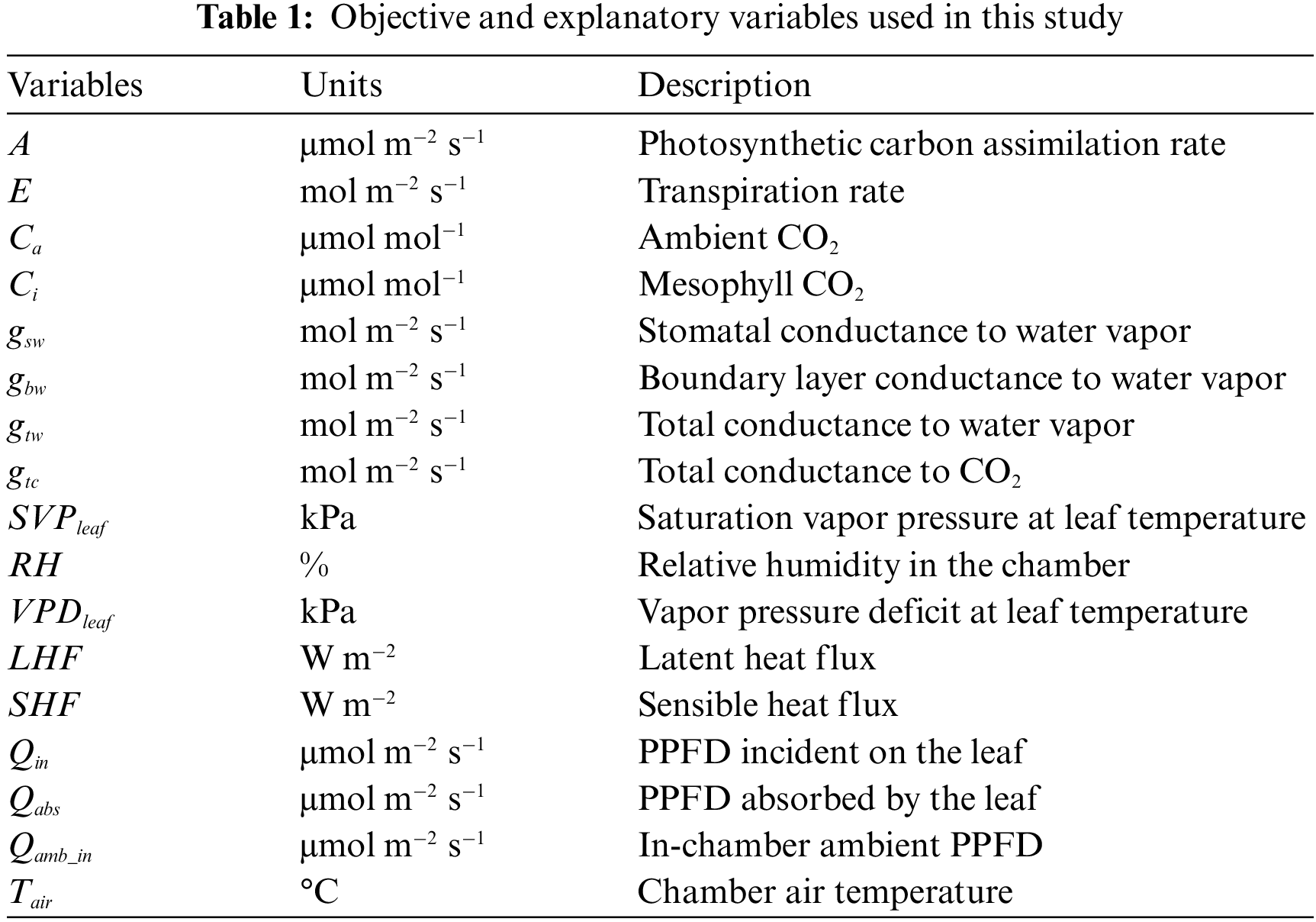
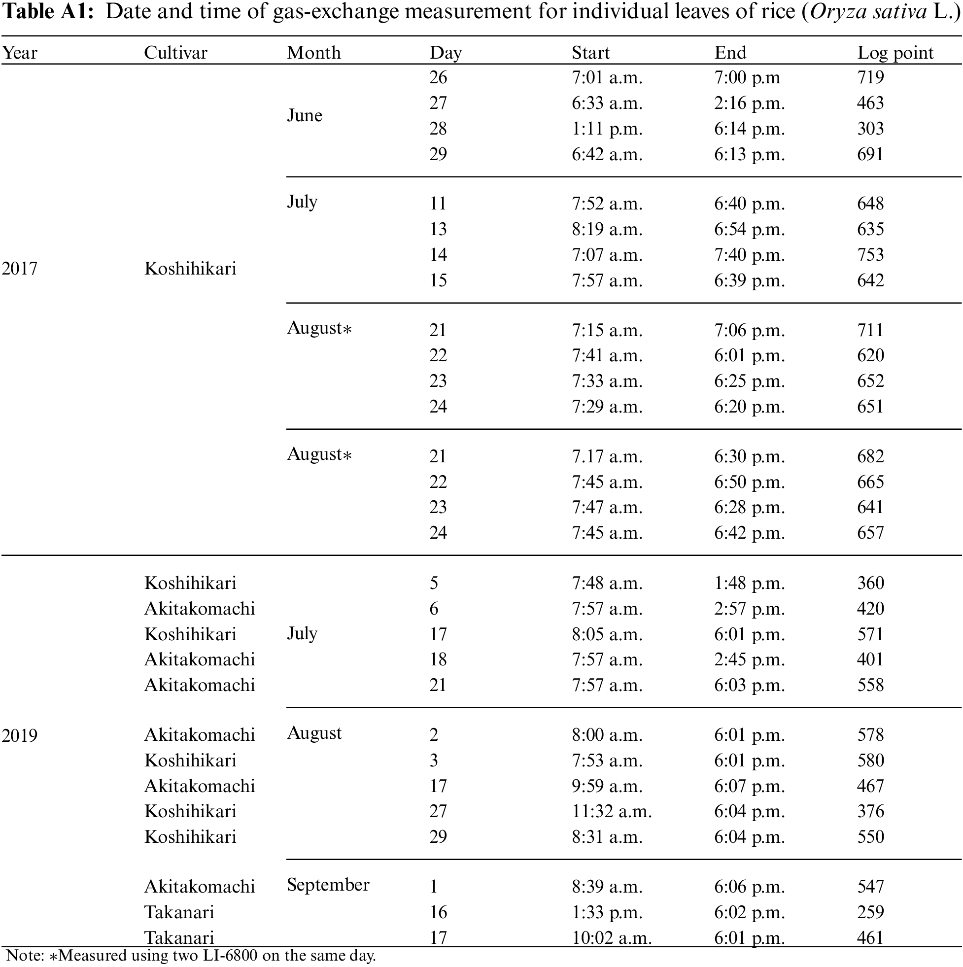
In this study, we performed gas-exchange measurements on individual leaves of three rice (Oryza Sativa L.) cultivars, “Koshihikari,” “Akitakomachi,” and “Takanari,” which were cultivated in 2017 and 2019 at the Field Museum Fuchu Honmachi paddy fields (139.47°E, 35.67°E), which are owned by the Field Science Center of the Tokyo University of Agriculture and Technology. A plant photosynthesis analysis system (LI-6800; LI-COR, Inc., NE, USA) was used for the measurements, for a total of 28 leaves (16 in 2017; 12 in 2019) when they were fully grown. Measurements were conducted from sunrise to sunset with samplings at 1-min intervals. Table A1 shows the measurement date, measurement start/end time, and the log score of each individual leaf. For the measurements, the LI-6800 light source was removed, and a fluctuating natural light was applied to the individual leaves in the chamber. The temperature and relative humidity in the chamber were measured hourly via a temperature/humidity meter (TR-72wb; T&D Corporation, Tokyo, Japan) that was installed near the field area and manually entered into the LI-6800 console. A, shown in Table 1, was used as the objective variable, and all others were used as explanatory variable candidates.

2.1 Data Pre-Processing

The outliers of the variables included in the measured data, as well as the different scales between variables, cause a loss of their characteristics and can have negative effects on the prediction accuracy of the constructed model. Therefore, it is necessary to pre-process and screen outliers prior to using values as model inputs and outputs. In this study, the mean μ and standard deviation σ values in the data that met the following conditional expressions in terms of the explanatory variable xt at time t in the gas-exchange measurement data were set as outliers.

|xt−μ|>2σ(1)

The outliers detected under the condition in Eq. (1) were first removed. Then, data interpolation was performed by a linear polynomial using the immediately preceding and immediately subsequent values.

An important technique when constructing a predictive model using machine learning is scaling for alignment by converting the values of the explanatory variables used for the input to the model according to a set standard. Scaling is performed to eliminate the effect of relatively small or large inputs that are strongly influenced by the predictive model. This is because the explanatory variables have numerical values of different magnitudes owing to their different units. In this study, scaling was performed using the following equation to eliminate the effect of the range of each explanatory variable on the model.

xstd=x−x¯σ(2)

Here, xstd is the value of each explanatory variable after standardization, x denotes the value of each explanatory variable before standardization, x¯ is the mean value of x, and σ is its variance. Applying Eq. (2) converts the mean to zero and the standard deviation to one, thereby scaling the dataset.

2.2 Variable Selection

General regression models have a multicollinearity problem, wherein increasing the regression coefficient's variance makes it unstable when there is a combination of explanatory variables with high correlation coefficients [29]. Therefore, it is recommended that either one of the explanatory variables with a high correlation coefficient be removed or the appropriate variables be selected [24]. Even the neural network behaves as a feature extractor that automatically extracts the important variables from the input; a combination of explanatory variables with extremely high correlations can make it difficult to properly capture the characteristics of patterns during learning. Furthermore, in terms of computational costs, it is desirable to appropriately select and reduce explanatory variables. In this study, the correlation coefficients at the same time point were determined for all explanatory variables shown in Table 1 (Fig. 1). According to the results, E, gtw, gtc, SVPleaf, VPDleaf, Qabs, and Qamb_in show highly positive and negative correlations with LHF, gsw, gsw, Tair, RH, Qin, and Qin. Therefore, these explanatory variables were excluded to avoid multicollinearity problems in the model. The latter group of variables adopted here had higher absolute correlation coefficient values with respect to the prediction target of A than the former group of variables.

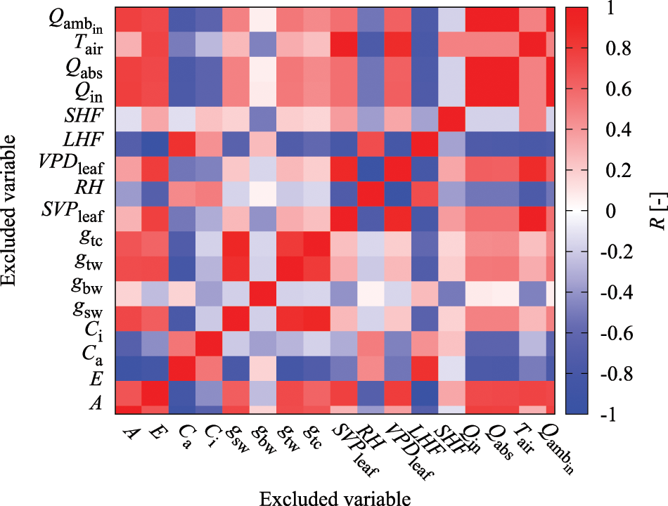
Figure 1: Color heatmap of correlation coefficient (R) between variables

2.3 Model Overview

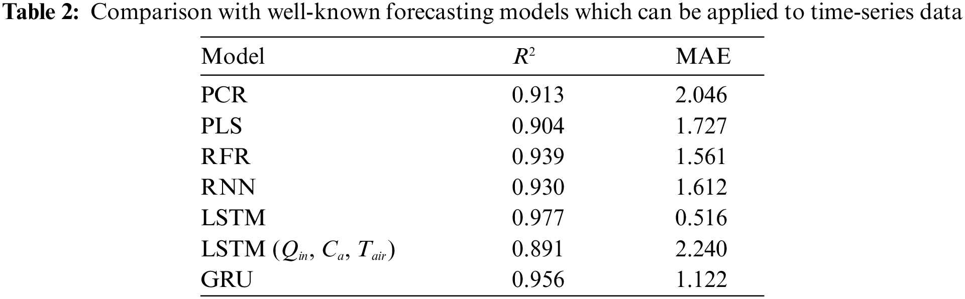
The predictive model of A for each rice leaf based on LSTM uses a prospective hidden layer to capture the long-term time-series characteristics of the explanatory variables. To confirm this property, we compared several regression models and other network architectures: principal component regression (PCR) [30], partial least-squares regression (PLS) [31], random forest regression (RFR) [32], basic recurrent neural network (RNN) [25], and gated recurrent units network (GRU) [33]. As shown in Table 2, LSTM showed the best accuracy when all variables selected in Section 2.2 were available. However, the accuracy decreased when using easy-to-measure variables listed as LSTM (Qin, Ca, Tair). Therefore, we tried to solve this problem by using a mechanism that generates variables that are effective for prediction from easy-to-measure variables. In the following sections, we provide details on LSTM and BALSTM.

2.3.1 LSTM and BLSTM

LSTM is a trainable model for long-term sequential data that is applied to solve problems such as long-term memory difficulty and gradient disappearance. LSTM has an information transmission architecture from past to present that resembles that of an RNN [34], but with a different transmission weighting format. Its most significant feature is that a hidden layer, called memory cell Ct, is inserted for state preservation in addition to weight matrix Ht, which is the previous node input. This helps avoid long-term memory and gradient disappearance (Fig. 2). LSTM includes forget gate ft, which is used to select content to maintain the memory, along with the input gates (it, gt) and output gate ot, which are used to control how new data are reflected or output at each time point as controllers for information propagation in the network. Its architecture is different from a simple RNN, which directly overwrites weights based on the state of the connected node. These gates are represented by four computational units that interact in a special architecture. Further, they contain a series of weights and activation functions, ft, it, gt, and ot, which are calculated as Eq. (3):

{ft=sigmoid (XtWX,f+Ht−1WH,f+bf)it=sigmoid(XtWX,i+Ht−1WH,i+bi)gt=tanh(XtWX,g+Ht−1WH,g+bg)ot=sigmoid (XtWX,o+Ht−1WH,o+bo)Ct=(Ct−1⊙ft)⊕(it⊙gt)Ht=ot⊙tanh⁡(Ct)(3)

Here, “sigmoid” is the sigmoid function, W denotes the vector parameter of the weight matrix to be trained, and b is the vector term of the bias. The operator ⊕ is the symbol for adding to the memory cell, and ⊙ is the pointwise product.

Memory cell Ct, which is defined by ft, it, and gt, adds the selected information after processing unnecessary information for the immediately preceding memory cell. The LSTM unit itself has a memory capacity with this series of memory control architectures, and the characteristics of long-term sequential data can be considered by using it in the intermediate layer and controlling the long-term information.

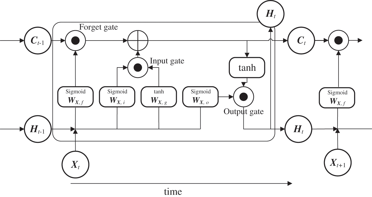
Figure 2: Basic structure of LSTM

Fig. 3 depicts an overview of the BLSTM model. RNNs, such as LSTM, normally handle the hidden state at t − 1 as an additional input in terms of the input at time t. Meanwhile, BLSTM adds LSTM as an intermediate layer, which operates in the opposite direction by handling the state at time t + 1 as an additional input with regard to the input at time t. BLSTM then makes predictions using both forward propagation into the future and backpropagation into the past. BLSTM uses future values for prediction at a certain point in time; therefore, its applications have been limited to fields such as machine translation [35], speech [36], and handwriting recognition [37,38]. This method was adopted in this study because the generated variables in the BLSTM module are all in the past time-series compared to the predicted time of A in the LSTM module, and therefore the real-time property of the model was not impaired.

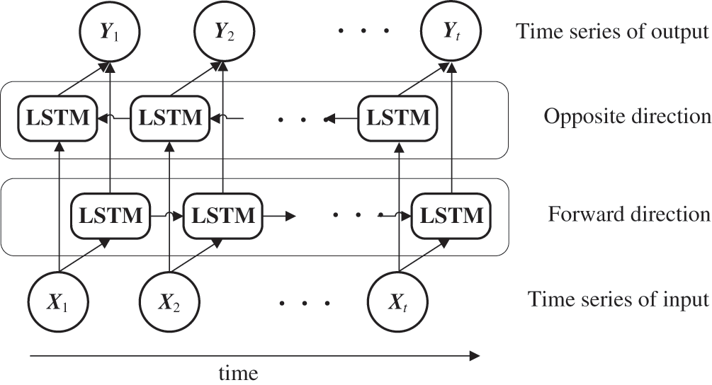
Figure 3: Unfolded BLSTM architecture

2.3.2 BLSTM-Augmented LSTM (BALSTM)

The explanatory variables used in the model should have low data acquisition costs and be easily measurable. Additionally, the practicality of the model would be greatly improved if only a few explanatory variables are used to reproduce the mesophyll variables and predict A. Meanwhile, as shown in Section 3.2, the prediction error of A when using only the external environment factors Qin, Ca, and Tair shown in Table 1, is relatively larger than the result of the model trained using all explanatory variables. Furthermore, screening tests for each explanatory variable suggest that fluctuations in Ci are important when determining A (Section 3.1). Therefore, the objective was to use the easy-to-calculate external environment variables for reproducing the mesophyll explanatory variables by augmentation architecture and to explicitly incorporate these values into LSTM for reproducing A using only external environment factors to improve its prediction accuracy.

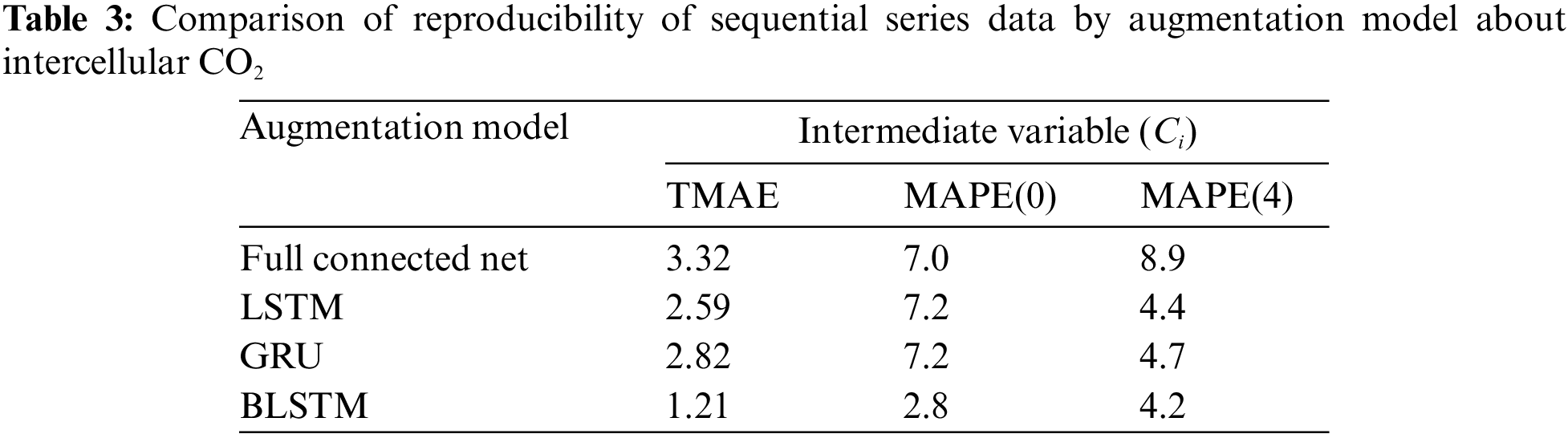
Fig. 4 shows an overview of the BALSTM model, which consists of two modules: one that reproduces the sequential data for the mesophyll variables, and one that predicts the photosynthetic carbon assimilation rate from the sequential data of the reproduced mesophyll variables and external environmental factors. The former uses BLSTM as the generative model to reproduce the sequential data of the mesophyll variables from the sequential data of the external environment variables. As shown in Table 3, we compared several neural network models that perform intermediate generation and found that BLSTM is the best candidate. Note that the input time-series variables and the generated time-series variables are at the same time. That is, the sequential mesophyll data, which are handled as explanatory variables in the LSTM model (see the previous section), were used as objective variables in the BALSTM model for training. The latter-predicted part of A included a combination of the sequential mesophyll data reproduced by BLSTM as an additional explanatory variable. Accordingly, predictions were made using LSTM.

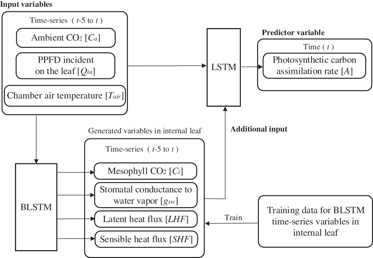
Figure 4: Basic structure of the BALSTM model

The BALSTM model is trained in two steps. First, the BLSTM model for augmentation is trained with the time-series variables of the external environmental factors as explanatory variables and the time-series variables of the leaf internals as objective variables. In the next step, the time-series variables of the leaf interior predicted using the trained BLSTM and the time-series variables of the external environmental factors are merged as the explanatory variables, and the objective variable, photosynthetic rate A, is trained using LSTM.

2.4 Model Validation

A total of 10,133 logs of actual measurement data from 2017 were used to develop the predictive model. However, the measurement period was long (approximately three months) and the temperature/light environment was variable. Therefore, A also fluctuated widely depending on the growth stage. Consequently, the predictive model could not be appropriately evaluated when fixing the validation data with the individual leaf data measured on a specific day because of its influence on training and testing. Thus, in this study, the nested cross-validation method [39] was used to evaluate the predictive model. Nested cross-validation is a method of validating a predictive model using bias elimination by transitioning the roles of the divided datasets for training, testing, and validation (Fig. 5).

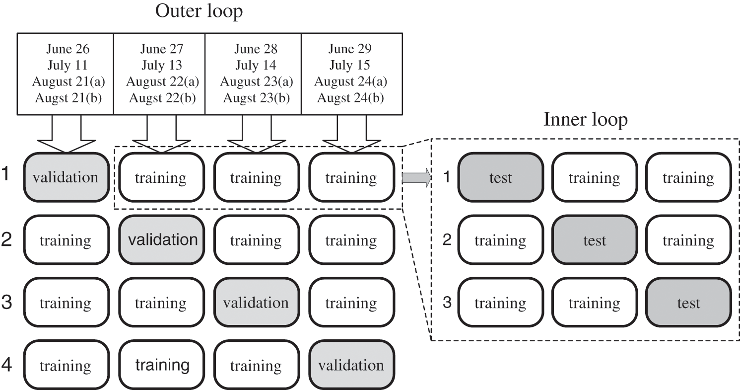
Figure 5: Nested cross-validation

First, all data obtained from the gas-exchange measurements were distributed. The individual leaf data of each month were evenly disseminated and separated into validation data and training data. The training data were then further divided into training data and test data. Training was performed using the training data, and the test data were used to search for the optimum values of the hyperparameters to minimize the learning error. In addition, they were employed to detect overfitting of training and to make early termination decisions. The predictive model was evaluated using the validation data. However, it was constructed by shifting the roles of the training and validation data to eliminate the bias influence of the training and adjustment data. Next, transitions of the validation data were conducted to eliminate the bias influence. The mean values of the evaluations for each validation data were used as the evaluated values of the final model. The time length in applying the sequential data for model accuracy validation in this study was set to 5 min. The predicted values were obtained for each sequential datum by moving it by 1 min (Fig. 6). The coefficient of determination (R2) and MAE were used to evaluate the predictive accuracy of A using the model.

Figure 6: Relationship between input and predicted values by the model

2.5 Evaluation of Mesophyll Variables Reproduced by BLSTM

The reproduced sequential data were evaluated by the following two methods to investigate their effect on sequential data predictions associated with the mesophyll variables reproduced in the BALSTM intermediate stage. First, the time-series mean absolute error (TMAE), which is expressed by the following equation for the overall performance of the reproduced time series, and the mean absolute percentage error (MAPE), which is used to evaluate each element of the reproduced time series, were calculated as Eqs. (4)–(6):

MAE=∑i=1n⁡|Oi−Pi|n(4)

TMAE=∑i=1mMAEm(5)

MAPE(t)=100m∑i=1m|Ot,i−Pt,iOt,i|(6)

Here, O is the measured value of the mesophyll variable obtained by the gas-exchange measurements, P is the value calculated by the model, n denotes the input width of the sequential data, m is the total sample size in the evaluated data, and t represents the tth element in the input width of the sequential data.

3  Results and Discussion

3.1 Effect of Explanatory Variables on Learning Model Prediction Accuracy

Neural network-based predictions and classifications produce remarkable results. However, researchers have been unable to explain their internal working mechanism because the trained model essentially matches statistical patterns, rendering it a black box. Some studies have quantitatively clarified the thought process underlying the answers produced by machine learning; nevertheless, there are presently no uniform solutions to this end. One approach for machine learning interpretability in the field of image classification is displaying an image area with a heat map [40]. Another approach that has received attention in the field of natural language processing visualizes the relationships between words [41]. However, few studies have been conducted on the quantitative interpretation of the results of learning models in the field of time-series predictive modeling. This is because of the strength of correlations before and after a time series and the difficulty of intuitive visualizations in image-related fields. In this study, the effects were visualized with a heat map when creating a predictive model by deleting the explanatory variables for each time series. Accordingly, the effect of each explanatory variable for training on the prediction of A was investigated. This approach is based on the hypothesis that prediction accuracy decreases when important explanatory variables are deleted during a predictive model development.

As a preliminary experiment, an LSTM prediction model was created using only a single explanatory variable to investigate the above hypothesis and to evaluate the prediction accuracy of A (Fig. 7). The results showed that R2 was approximately 0.8 with Qin and Ca only, and a relatively high prediction accuracy was obtained.

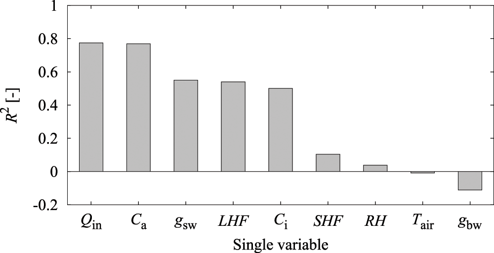
Figure 7: Accuracy of reproduction of assimilation rate (A) by a single variable

Fig. 8 shows the effect on the prediction accuracy when the explanatory variables are excluded during the LSTM learning model construction. The vertical axis denotes the excluded variable, and the horizontal axis represents the prediction result of A up to 60 min ahead in 5-min intervals. The effect of the excluded variable was quantified by developing a prediction model with the remaining variables after excluding the explanatory variable on the vertical axis. The R2 values were then calculated and standardized to make each column have a mean of zero and a variance of one. In other words, excluded variables that have a significant effect on the prediction accuracy are deemed important in the blue region, whereas the relatively unimportant variables are shown in the red region.

Figure 8: Influence of explanatory variables for each prediction time on prediction accuracy by LSTM

As shown in Fig. 8, Ca, Ci, gsw, and gbw are important variables for improving the prediction accuracy at least 60 min ahead. It can also be observed in the prediction of the current values that Ci is the most important variable for determining A. Moreover, from the preliminary calculations, it is evident that the reproducibility of the LSTM model using only Ci is lower than that using Qin or Ca. Therefore, a high reproducibility may be achieved because of the influence of Ci fluctuations along with other variables. This can be explained by the fact that A is proportional to the difference between the internal and external CO2 concentrations. Meanwhile, Qin, which is the most important explanatory variable in the preliminary calculation, is less important in the LSTM model for all explanatory variables. This is believed to be because the effects of Qin are reflected in other explanatory variables, resulting in its relatively smaller influence. Further, it can be observed that the sequential values of Ca and Ci continue to have a strong influence on the prediction accuracy of A up to 60 min ahead.

3.2 Model Prediction Accuracy

Excluding the external environment variables, Ci, gsw, LHF, and RH exerted, in descending order, a larger influence on the predictive model with regard to the current value predictions of A by LSTM (Section 3.1). First, LSTM prediction accuracy values were calculated using all explanatory variables. Then, LSTM (Qin, Ca, Tair) values were predicted by only the external environment variables Qin, Ca, and Tair. BALSTM (Qin, Ca, Tair), which were calculated by the same external environment variables, reproduce and utilize mesophyll variables Ci, gsw, LHF, and RH via BLSTM. Note that the reproduced variable is represented as a subscript. The accuracy of each method was compared. The results showed that, excluding LSTM with all variables, the best prediction accuracy was for BALSTMCi,gsw(Qin, Ca, Tair), which generated and used Ci and gsw (Table 4). Meanwhile, the reproduction accuracy values of BALSTMCi,gsw,LHF, BALSTMCi,gsw,LHF,RH, and BALSTMgsw,LHF,RH, which were obtained by adding LHF and RH and generating three or more variables, did not improve compared to BALSTMCi,gsw. This is because the training parameters increased with an increase in the number of prediction targets, making the training of the entire model difficult. Furthermore, the data with a low importance and low accuracy were input to the LSTM, thereby predicting A as noise. However, improving the prediction accuracy of A may be possible if the mesophyll variables can be reproduced with high accuracy using a wider range of training data and model improvements. Furthermore, the TMAE values of the mesophyll variables were as follows: Ci = 1.21–1.32 μmol mol−1 and gsw = 0.055–0.077 mol m−2 s−1. For MAPE(0), the values were as follows: Ci = 2.8%–3.2% and gsw = 2.2%–3.3%. For MAPE(4), the values were as follows: Ci = 4.2%–7.1% and gsw = 6.3%–7.6% (Table 4). The initial stage of the input time series (i.e., MAPE(0)) could be reproduced with a higher accuracy than a later prediction point (i.e., MAPE(4)), is because the initial values of the time series to be reproduced were generated using future values on account of the BLSTM characteristics (Fig. 4). The advantage of this characteristic is evident from the comparison of the augmentation models shown in Table 4.

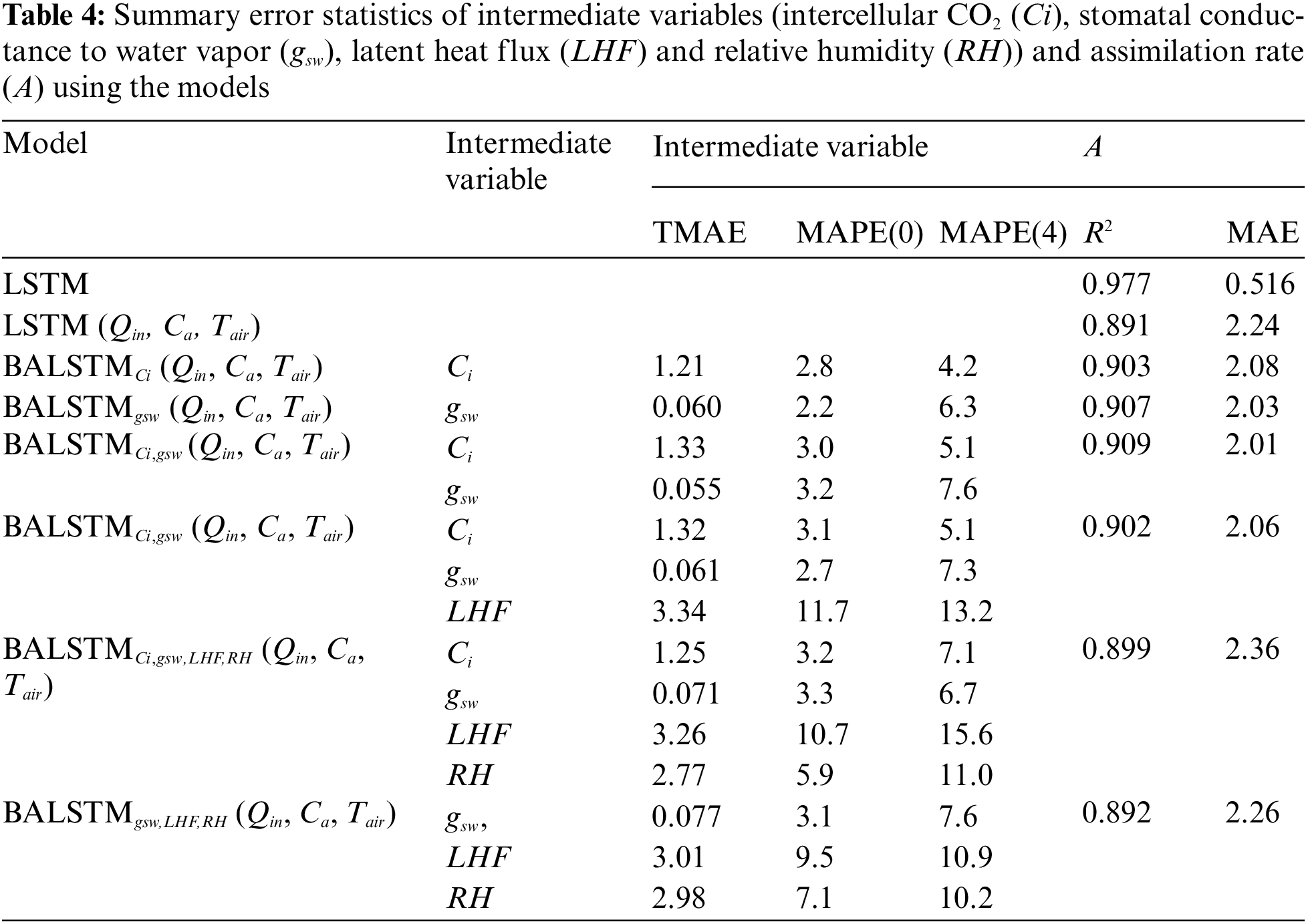
Fig. 9 shows the prediction accuracy of A up to 60 min. This figure shows how the prediction accuracy of A changes by entering the values of the explanatory variables during a 5-min period into the trained model, thereby predicting the value from that time to a lead time of 60 min at 5-min intervals. Moreover, it is repeated with a time step of 1 min, and the measured and predicted values are compared. LSTM had the best prediction accuracy for 60-min-ahead predictions based on the MAE index, compared with LSTM (Qin, Ca, Tair) and BALSTMCi,gsw. Meanwhile, BALSTMCi,gsw had a smaller prediction error than LSTM(Qin, Ca, Tair) in terms of the MAE index. In terms of the R2 index, the 20-min-ahead prediction by BALSTMCi,gsw was less accurate than that by LSTM; however, the prediction value after 20 min was better than that of LSTM.

Figure 9: Relationship between prediction time and prediction accuracy of A with each model: (a) MAE and (b) R2

These findings suggest that BALSTMCi,gsw plays an important role in preventing a decline in prediction accuracy by considering the sequential characteristics of the mesophyll variables, especially for predicting A 20 min in advance. These findings also show that the time-series values of the mesophyll variables reproduced by BLSTM contributed to improving the prediction accuracy of A, even for prediction times up to 20 min ahead. These results suggest that prior knowledge of the mesophyll environment has a significant influence on the prediction of A.

3.3 Effect of Sequential Data Length in Model Input on Prediction of Photosynthetic Carbon Assimilation Rate

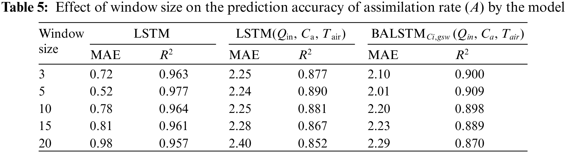
The time-series length of the input data used in this study's prediction model was 5 min. This is because highly accurate predictions could be made without setting the window size of the sequential data to over 5 min when predicting the current value of A by LSTM (Table 5). Furthermore, whether a prior history of the external environment influences the prediction accuracy was investigated for LSTM (Qin, Ca, Tair) and BALSTMCi,gsw. The results showed that both LSTM (Qin, Ca, Tair) and BALSTMCi,gsw had the highest accuracy when the time-series length was 5 min, and the accuracy decreased when the input width was increased. By contrast, the decrease in accuracy was minimal when the window size of the time series was reduced to 3 min. The above results show that important information was concentrated in the latest value for the prediction of A, and they show the appropriate window size for capturing the dynamic characteristics of A from the time-series information of external variables using LSTM, LSTM (Qin, Ca, Tair), and BALSTMCi,gsw (Qin, Ca, Tair). By contrast, increasing the window size increased the model complexity and decreased the prediction accuracy.

3.4 Model Generalization and Applicability

Fig. 10 and Table 6 show the results of predicting A using the dataset of gas-exchange measurements of each individual leaf in FY2019 (Table A1) by applying the model trained with the FY2017 dataset. According to the results, three categories could be classified relative to LSTM (Qin, Ca, Tair) (Table 6): the case where errors significantly decreased because of BALSTMCi,gsw incorporating Ci and gsw as intermediate product variables (Fig. 10a), the case where errors were almost unchanged in both models and the prediction accuracy was generally satisfactory (Fig. 10b), and the case where the absolute error was large for both models and the prediction accuracy was low (Fig. 10c).

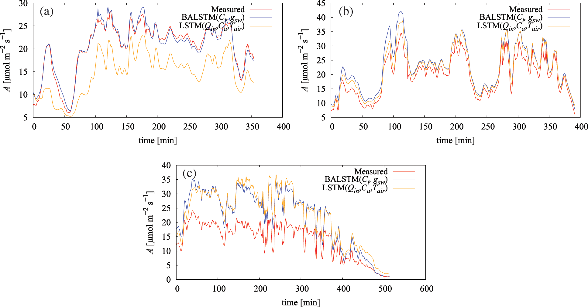
Figure 10: Measured and simulated assimilation rate (A): (a) July 5, 2019, (b) July 18, 2019, and (c) July 17, 2019

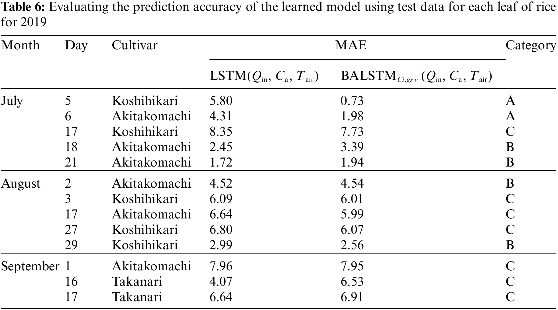
The use of BALSTMCi,gsw enabled both the reproduction of Ci and gsw and the confirmation of samples in which the prediction accuracy of A was significantly improved (Category A in Fig. 11 and Table 6). Meanwhile, the accuracy of BALSTMCi,gsw is not always excellent in each Category B sample in Table 6. These results suggest that accuracy was improved in samples for which sufficient accuracy could not be obtained only with external environment variables by reproducing the mesophyll variables with BALSTM and by using them as explanatory variables for the prediction. Additionally, half of the samples in Table 6 have relatively lower prediction accuracies of A for both LSTM (Qin, Ca, Tair) and BALSTMCi,gsw (Qin, Ca, Tair) when comparing Categories A and B. As shown in Fig. 12, the data distribution of the external environment variables of the samples classified as Category C shows that the photosynthetic photon flux and temperature in the summer were higher than those in the training data. The prediction accuracy was also low for “Takanari,” whose strains are different from those of “Koshihikari” and “Akitakomachi,” neither of which were used to train the models. Therefore, there remain certain unresolved issues for making predictions using input data outside the numerical range of training data, such as time, cultivars, and growth stage, and for applying them to models of cultivars not used in learning. Meanwhile, Ci and gsw in the mesophyll can be reproduced in addition to predicting A if BALSTMCi,gsw is used; thus, we can assume that both Ci and gsw can be reproduced and A can be predicted based on various external environment scenarios using a wide range of gas-exchange measurement data as the training data for machine learning models in the future.

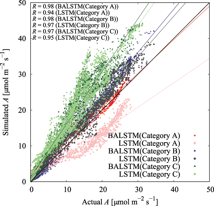
Figure 11: Residual plot of assimilation rate (A) in each category in Table 6

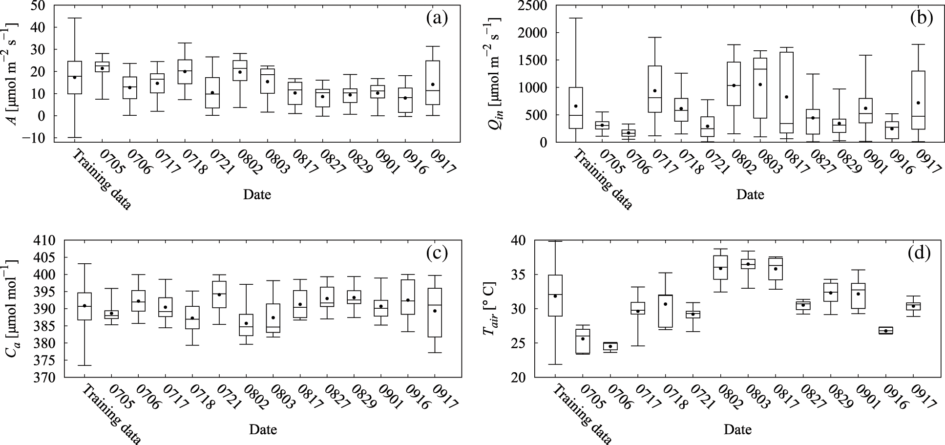
Figure 12: Box plots of variable values for training data and each leaf for measurements in 2019: (a) assimilation rate (A), (b) PPFD incident on the leaf (Qin), (c) ambient CO2 (Ca), and (d) chamber air temperature (Tair)

The meteorological environment in the closed chamber used in this study was significantly different from the field environment, except for the light environment. The target cultivar used for learning was “Koshihikari,” and only the most developed leaves were used for measuring the leaf positions. Therefore, measured values under various conditions, such as the cultivar, soil conditions, fertilization conditions, growth stage, and leaf position, are needed to make the proposed model more robust. Furthermore, applying this technology to the prediction of canopy-scale photosynthesis in the field requires detailed investigations on the historical effect of the meteorological environment on the photosynthetic carbon assimilation rate A of individual leaves. It also requires the accumulation of knowledge through experimental and theoretical studies, such as connections with a precise prediction model of micrometeorology, including the area's vertical direction. We believe that solving these problems would enable an accurate prediction of canopy growth and dry matter production, as well as the acquisition of a large amount of phenotypic data of crops that affect growth using a prediction model. This determination can provide a perspective on which phenotypes should be targeted when breeding for efficiency and speed.

4  Conclusions

This study focused on predicting the photosynthetic carbon assimilation rate A of individual rice leaves. BALSTM was used to construct a predictive model of A and to verify its accuracy. The most significant feature of BALSTM is its hybrid architecture, where Ci and gsw are reproduced as intermediate products in addition to A using only the easy-to-measure environmental variables of Qin, Ca, and Tair. The obtained output is then added to the training model. The results showed the following: 1) BALSTMCi,gsw (Qin, Ca, Tair) had a significantly higher prediction accuracy than LSTM (Qin, Ca, Tair); 2) the hybrid model with Ci and gsw as intermediate products had a higher accuracy in reproducing A than the other combinations of intermediate products; 3) the MAPE values in the reproduction of Ci and gsw were 5.1% and 7.6%, respectively, with good results overall; and 4) having a mechanism to reproduce the mesophyll variables improved the reproduction and prediction accuracy of A when compared with only using the external environment variables. In the future, we intend to conduct gas-exchange measurements that include a wider range of external environment variables, build a robust model by increasing the amount of data required for model learning, and improve the model's prediction accuracy. We will also strive to build an information infrastructure that can be applied to the decision-making of on-site agricultural work by combining spatial wide-area information, such as remote sensing data, with the relatively easy-to-measure external environment as an explanatory variable. Finally, we will spatiotemporally extend the application of BALSTM and simultaneously construct a system to predict A in real time.

Acknowledgement: We thank Prof. Nguyen Tuan Cuong and Prof. Nguyen Tuan Hung from the Tokyo University of Agricultural and Technology, Japan, for their support with data analysis.

Availability of Data and Materials: The data that support the findings of this study are available from the corresponding author upon reasonable request.

Funding Statement: The authors gratefully acknowledge the support of JST PRESTO (Grant No. JPMJPR16O3) and JSPS KAKENHI (Grant Nos. 16KK0169 and 19K15944).

Conflicts of Interest: The authors declare that they have no conflicts of interest to report regarding the present study.

References

 1.  Hall, D. O. (1977). Photosynthesis-A practical energy source? In: Castellani, A. (Ed.Research in photobiology, pp. 347–359. USA: Springer. DOI 10.1007/978-1-4613-4160-4_36. [Google Scholar] [CrossRef]

 2.  Shipley, B., Vile, D., Garnier, E., Wright, I. J., Poorter, H. (2005). Functional linkages between leaf traits and net photosynthetic rate: Reconciling empirical and mechanistic models. Functional Ecology, 19, 602–615. DOI 10.1111/j.1365-2435.2005.01008.x. [Google Scholar] [CrossRef]

 3.  Caemmerer, S. V. (2000). Biochemical models of leaf photosynthesis. Techniques in Plant Science, Collingwood: CSIRO. [Google Scholar]

 4.  Farquhar, G. D., von Caemmerer, S., Berry, J. A. (1980). A biochemical model of photosynthetic CO2 assimilation in leaves of C3 species. Planta, 149, 78–90. DOI 10.1007/BF00386231. [Google Scholar] [CrossRef]

 5.  Glime, J. M. (2007). Bryophyte ecology. In: Physiological ecology, vol. 1. Houghton, Michigan, U.S., Michigan Technological University and the International Association of Bryologists. [Google Scholar]

 6.  Carmo-Silva, E., Scales, J. C., Madgwick, P. J., Parry, M. A. J. (2015). Optimizing rubisco and its regulation for greater resource use efficiency. Plant Cell Environment, 38, 1817–1832. DOI 10.1111/pce.12425. [Google Scholar] [CrossRef]

 7.  Lawson, T., Kramer, D. M., Raines, C. A. (2012). Improving yield by exploiting mechanisms underlying natural variation of photosynthesis. Current Opinion in Biotechnology, 23, 215–220. DOI 10.1016/j.copbio.2011.12.012. [Google Scholar] [CrossRef]

 8.  Naumburg, E., Ellsworth, D. S. (2002). Short-term light and leaf photosynthetic dynamics affect estimates of daily understory photosynthesis in four tree species. Tree Physiology, 22, 393–401. DOI 10.1093/treephys/22.6.393. [Google Scholar] [CrossRef]

 9.  Poorter, H., Fiorani, F., Pieruschka, R., Wojciechowski, T., Putten, W. H. et al. (2016). Pampered inside, pestered outside? Differences and similarities between plants growing in controlled conditions and in the field. New Phytologist, 212, 838–855. DOI 10.1111/nph.14243. [Google Scholar] [CrossRef]

10. Sakoda, K., Yamori, W., Groszmann, M., Evans, J. R. (2021). Stomatal, mesophyll conductance, and biochemical limitations to photosynthesis during induction. Plant Physiology, 185, 146–160. DOI 10.1093/plphys/kiaa011. [Google Scholar] [CrossRef]

11. Slattery, R. A., Walker, B. J., Weber, A. P. M., Ort, D. R. (2018). The impacts of fluctuating light on crop performance. Plant Physiology, 176, 990–1003. DOI 10.1104/pp.17.01234. [Google Scholar] [CrossRef]

12. Sun, J., Ye, M., Peng, S., Li, Y. (2016). Nitrogen can improve the rapid response of photosynthesis to changing irradiance in rice (Oryza sativa L.) plants. Science Reporter, 6, 31305. DOI 10.1038/srep31305. [Google Scholar] [CrossRef]

13. Vialet-Chabrand, S., Matthews, J. S. A., Simkin, A. J., Raines, C. A., Lawson, T. (2017). Importance of fluctuations in light on plant photosynthetic acclimation. Plant Physiology, 173, 2163–2179. DOI 10.1104/pp.16.01767. [Google Scholar] [CrossRef]

14. Andrew, R. C., Malekian, R., Bogatinoska, D. C. (2018). IoT solutions for precision agriculture. Proceedings of the 41st International Convention on Information and Communication Technology, Electronics and Microelectronics (MIPRO), pp. 345–349. Rijeka, Croatia. [Google Scholar]

15. García, L., Parra, L., Jimenez, J. M., Lloret, J., Lorenz, P. (2020). IoT-based smart irrigation systems: An overview on the recent trends on sensors and IoT systems for irrigation in precision agriculture. Sensors, 20, 1042. DOI 10.3390/s20041042. [Google Scholar] [CrossRef]

16. Jha, K., Doshi, A., Patel, P., Shah, M. (2019). A comprehensive review on automation in agriculture using artificial intelligence. Artificial Intelligence in Agriculture, 2, 1–12. DOI 10.1016/j.aiia.2019.05.004. [Google Scholar] [CrossRef]

17. Mohapatra, A. G., Keswani, B., Lenka, S. K. (2018). ICT specific technological changes in precision agriculture environment. International Journal of Computer Science and Mobile Computing, 6, 1–16. [Google Scholar]

18. Sreekantha, D. K., Kavya, A. M. (2017). Agricultural crop monitoring using IOT-a study. 2017 11th International Conference on Intelligent Systems and Control (ISCO), pp. 134–139. Coimbatore, India. DOI 10.1109/ISCO.2017.7855968. [Google Scholar] [CrossRef]

19. Liakos, K., Busato, P., Moshou, D., Pearson, S., Bochtis, D. (2018). Machine learning in agriculture: A review. Sensors, 18, 2674. DOI 10.3390/s18082674. [Google Scholar] [CrossRef]

20. Lü, W., Li, Y. H., Mao, W. B., Gong, X., Chen, S. G. (2017). Comparison of estimation methods for net photosynthetic rate of wheat's flag leaves based on hyperspectrum. Journal of Agricultural Resources and Environment, 34, 582–586. DOI 10.13254/j.jare.2017.0173. [Google Scholar] [CrossRef]

21. Heckmann, D., Schlüter, U., Weber, A. P. M. (2017). Machine learning techniques for predicting crop photosynthetic capacity from leaf reflectance spectra. Molecular Plant, 10, 878–890. DOI 10.1016/j.molp.2017.04.009. [Google Scholar] [CrossRef]

22. Zhang, X. Y., Huang, Z., Su, X., Siu, A., Song, Y. et al. (2020). Machine learning models for net photosynthetic rate prediction using poplar leaf phenotype data. PLoS One, 15, e0228645. DOI 10.1371/journal.pone.0228645. [Google Scholar] [CrossRef]

23. Greff, K., Srivastava, R. K., Koutnik, J., Steunebrink, B. R., Schmidhuber, J. (2017). LSTM: A search space odyssey. IEEE Transactions on Neural Networking and Learning Systems, 28, 2222–2232. DOI 10.1109/TNNLS.2016.2582924. [Google Scholar] [CrossRef]

24. Hochreiter, S., Schmidhuber, J. (1997). Long short-term memory. Neural Computation, 9, 1735–1780. DOI 10.1162/neco.1997.9.8.1735. [Google Scholar] [CrossRef]

25. Sherstinsky, A. (2020). Fundamentals of recurrent neural network (RNN) and long short-term memory (LSTM) network. Physica D: Nonlinear Phenomena, 404, 132306. DOI 10.1016/j.physd.2019.132306. [Google Scholar] [CrossRef]

26. Graves, A., Schmidhuber, J. (2005). Framewise phoneme classification with bidirectional LSTM and other neural network architectures. Neural Networks, 18, 602–610. DOI 10.1016/j.neunet.2005.06.042. [Google Scholar] [CrossRef]

27. Hayashi, T., Watanabe, S., Toda, T., Hori, T., Roux, J. L. et al. (2017). BLSTM-HMM hybrid system combined with sound activity detection network for polyphonic sound event detection. 2017 IEEE International Conference on Acoustics, Speech and Signal Processing (ICASSP), pp. 766–770. New Orleans, LA, USA. DOI 10.1109/ICASSP.2017.7952259. [Google Scholar] [CrossRef]

28. Schuster, M., Paliwal, K. K. (1997). Bidirectional recurrent neural networks. IEEE Transactions on Signal Processing, 45, 2673–2681. DOI 10.1109/78.650093. [Google Scholar] [CrossRef]

29. Kuhn, M., Johnson, K. (2013). Applied predictive modeling. USA: Springer. DOI 10.1007/978-1-4614-6849-3. [Google Scholar] [CrossRef]

30. Xie, Y. L., Kalivas, J. H. (1997). Evaluation of principal component selection methods to form a global prediction model by principal component regression. Analytica Chimica Acta, 348, 19–27. DOI 10.1016/S0003-2670(97)00035-4. [Google Scholar] [CrossRef]

31. Rosipal, R., Krämer, N. (2005). Overview and recent advances in partial least squares. The International Statistical and Optimization Perspectives Workshop “Subspace, Latent Structure and Feature Selection”, pp. 34–51. Berlin, Heidelberg. DOI 10.1007/11752790_2. [Google Scholar] [CrossRef]

32. Chen, C., Liaw, A., Breiman, L. (2004). Using random forest to learn imbalanced data, browsed on Aug. 4, 2020. [Google Scholar]

33. Chung, J., Gulcehre, C., Cho, K., Bengio, Y. (2014). Empirical evaluation of gated recurrent neural networks on sequence modeling. NIPS 2014 Workshop on Deep Learning, Montréal, Canada. https://arxiv.org/abs/1412.3555. [Google Scholar]

34. Rumelhart, D. E., Hinton, G. E., Williams, R. J. (1986). Learning representations by back-propagating errors. Nature, 323, 533–536. DOI 10.1038/323533a0. [Google Scholar] [CrossRef]

35. Bahdanau, D., Cho, K., Bengio, Y. (2016). Neural machine translation by jointly learning to align and translate. https://doi.org/10.48550/arXiv.1409.0473 [Google Scholar]

36. Graves, A., Mohamed, A., Hinton, G. (2013). Speech recognition with deep recurrent neural networks. International Conference on Acoustics, Speech and Signal Processing (ICASSP), pp. 6645–6649. Vancouver, BC, Canada. DOI 10.1109/ICASSP.2013.6638947. [Google Scholar] [CrossRef]

37. Ly, N. T., Nguyen, C. T., Nakagawa, M. (2020). An attention-based row-column encoder-decoder model for text recognition in Japanese historical documents. Pattern Recognition Letters, 136, 134–141. DOI 10.1016/j.patrec.2020.05.026. [Google Scholar] [CrossRef]

38. Nguyen, H. T., Nguyen, C. T., Bao, P. T., Nakagawa, M. (2018). A database of unconstrained Vietnamese online handwriting and recognition experiments by recurrent neural networks. Pattern Recognition, 78, 291–306. DOI 10.1016/j.patcog.2018.01.013. [Google Scholar] [CrossRef]

39. Raschka, S. (2020). Model evaluation, model selection, and algorithm selection in machine learning. arXiv:1811.12808. [Google Scholar]

40. Selvaraju, R. R., Cogswell, M., Das, A., Vedantam, R., Parikh, D. et al. (2020). Grad-CAM: Visual explanations from deep networks via gradient-based localization. International Journal of Computing Vision, 128, 336–359. DOI 10.1007/s11263-019-01228-7. [Google Scholar] [CrossRef]

41. Vaswani, A., Shazeer, N., Parmar, N., Uszkoreit, J., Jones, L. et al. (2017). Attention is all you need. Proceedings of the 31st International Conference on Neural Information Processing Systems (NIPS17), pp. 6000–6010. Long beach, California, USA. [Google Scholar]

Appendix

This work is licensed under a Creative Commons Attribution 4.0 International License, which permits unrestricted use, distribution, and reproduction in any medium, provided the original work is properly cited.