Computer Modeling in Engineering & Sciences

---

DOI: 10.32604/cmes.2022.021865

ARTICLE

Regarding Deeper Properties of the Fractional Order Kundu-Eckhaus Equation and Massive Thirring Model

Yaya Wang1, P. Veeresha2, D. G. Prakasha3, Haci Mehmet Baskonus4,* and Wei Gao5

1Department of Information Engineering, Binzhou Polytechnic, Binzhou, 256603, China
2Centre for Mathematical Needs, Department of Mathematics, CHRIST (Deemed to be University), Bengaluru, 560029, India
3Department of Mathematics, Davangere University, Shivagangothri, Davangere, 577007, India
4Department of Mathematics and Science Education, Faculty of Education, Harran University, Sanliurfa, 63050, Turkey
5School of Information Science and Technology, Yunnan Normal University, Kunming, 650500, China
*Corresponding Author: Haci Mehmet Baskonus. Email: hmbaskonus@gmail.com
Received: 10 February 2022; Accepted: 11 April 2022

1  Introduction

The study of complex models that exemplify the nonlinear phenomena and analyze their behaviour is essential and pivotal in the research of the present era. Particularly, the role of mathematics is significant to illustrate their nature with respect to time and other dependent parameters. The essence of calculus and its applications have become a hot topic from the beginning of its birth to till date. Since it is only instrument which can effectively and accurately predict the behaviour of the process raised in nature as a problem for living beings or solutions for the same. Recently, many pioneers and young researchers pointed out some limitations while designing or modelling complicated phenomena with classical calculus. Specifically, while examining hereditary properties, history-based mechanisms, non-Morkian processes, long-range propagations and others. Meanwhile, on the other hand the concept of calculus with non-integer order is rooted soon after the classical one in the process of the letter exchange between two great mathematicians. During the seventeenth and eighteenth centuries, this concept was not gets attracted by numerous scholars due to the unfamiliarity of its essence and associated applications in comparison with classical concepts. But, recently, due to the above cited boundaries of integer order calculus and revolution in the computational tools, the concept of fractional calculus (FC) fascinates many physicists, engineers and most importantly, mathematicians to develop the essential theory and corresponding computational tools deal with the real-world problem for the betterment of lifestyle of the human beings. Many senior scholars provided the base for the FC in order to understand in scientific needs of implementing this concept into reality [1–6].

Recently, many existed models have been examined by researchers [7–10]. For instance, the new wave behavior of the equations exemplifying the phenomena associated with plasma physics is derived by researchers in [11], the scholars in [12] derived stimulating results associated with a numerical method for coupled KdV equations. The efficient approach is employed in [13] to model for thermostats with hybrid boundary value conditions, the reliability of the method is illustrated by researchers in [14] with respect to the (2+1)-dimensional Ablowitz-Kaup-Newell-Segur equation, the prey models with mutualistic predation is analyzed in [15] with the help of non-local and non-singular kernels. In a similar manner, the authors in [16–18] derived some interesting results associated with numerical methods. Moreover, the authors in [19] investigated the model that exemplifies the wind-influenced projectile motion within the frame of fractional calculus. In [20], researchers illustrated the impact of the generalization of the classical model with arbitrary models. These studies motivate us to investigate more complex models with the help of efficient numerical or analytical methods and aid us in investigating comparative numerical study. On the other hand, the following recent research work helps us to understand the essence of generalizing the concept with fractional order. For instance, the author in [21] derived the two Fibonacci operational matrix pseudo-spectral schemes to investigate the physical model, the researchers in [22] studied the SIR model of the current 2019-nCoV with Caputo operator, the complex nature of the Gross–Pitaevskii equations derived with the help of fractional derivative. Further, many scholars employed different fractional operators to analyze real-world problems and study the physical phenomena [23–28], for instance, COVID-19 in India [29], biological pest control in tea plants [30], and many others.

In the present investigation, the model exemplifying important phenomena in quantum field theory is considered. The nonlinear Schrödinger (NLS) equation plays a vivacious part in the study of nonlinear optics, photonics, quantum field theory, water wave, and others. Among such, the Kundu-Eckhaus (KE) equation and the massive Thirring model (MTM) are the most important models and describe the self-interactions of a Dirac field. In the 1980’s, Kundu [31] and Eckhaus et al. [32,33] proposed the Kundu-Eckhaus equation as a linearizable form of the NLS equation. Here, we considered the fractional Kundu-Eckhaus (FKE) equation and fractional massive Thirring model (FMTM). The fractional-order is presented to incorporate the memory consequences in the system, which aids in capturing the essential behaviour of the complex model as follows [34]. The FKE equation

iDtμu(x,t)+uxx(x,t)+2u(x,t)(|u(x,t)|2)x+u(x,t)|u(x,t)|4=0,0<μ≤1,(1)

with u(x,0)=αeix. The FMTM equations are given by

{i(Dtμu(x,t)+ux(x,t))+v(x,t)+u(x,t)|v(x,t)|2=0,i(Dtμv(x,t)+vx(x,t))+u(x,t)+v(x,t)|u(x,t)|2=0,0<μ≤1,(2)

with u(x,0)=αeix and v(x,0)=βeix.

where u(x,t) and v(x,t) are the complex smooth envelop function of temporal (t) and spatial (x) variables, i is the imaginary number (i.e., i=−1) and μ is the arbitrary order. Authors in [35] illustrated that Kundu-Eckhaus and the complex Burgers equations are associated with a Miura transformation. The KE equation can effectively model the propagation of ultra short pulses in quantum and nonlinear optics, which can be employed to illustrate the optical properties of the fem to second lasers and helps to study the behaviour of different phenomena arising into chemistry. Further, the massive Thirring model (MTM) is the nonlinear complex system having two-component [36,37]. This model is used to illustrate the propagation of optical pulse in nonlinear or periodic optical media. Much attention has been devoted to the connection between the quantum sine-Gordon model and the quantum Thirring model [38,39]. This association helps the considered problem to describe the model either in accordance with perturbation theory or in accordance with ordinary perturbation theory for quantum solitons.

As much as real-world modelling problems are important, finding the solution for these models with differential equations is also important. With the help of literature, we can say that, every model does not process an exact solution. In this regard, researchers employed or aided by semi-analytical or numerical algorithms. In this connection, Adomian offered the Adomian decomposition method (ADM) [40], particularly to examine nonlinear systems. With the help of the Adomian polynomial, we can solve nonlinear terms in a simple form. Even though a wide community of researchers applied to study many physical and other problems, recently, many scholars showed that if this method is union with transformation leads the great efficiency accuracy and reduces time and computational work. To fulfil these necessities, Rawashdeh et al. proposed the FNDM [41,42], and it is a mixture of ADM and natural transform. From the lost three years, this projected scheme is applied by many researchers to examine many problems and systems [43–46].

The pivotal aim of the present work is to find a solution for the FKE equation and FMT model and study the behaviour of the obtained solutions with respect to fractional order. Since these equations play an important role in describing various complex phenomena, many authors find and analyzed the solution numerically as well as analytically. For instance, authors in [47] found the rogue-wave solutions in optical fiber for KE equation, and auxiliary equation expansion and modified unified algebraic techniques are considered in order to find the soliton solution for KE equation. Further, many efficient techniques are applied to analyze these equations, modified simple equation scheme [48], extended trial function method [49], q-homotopy analysis transform technique [39], and many techniques for KE and MTM equations having classical and fractional order derivatives [50–55].

2  Preliminaries

Here, we present the essential and basic notions of FC and natural transform.

Definition 1. The fractional order Riemann-Liouville integral of a function f(t)∈Cδ(δ≥−1) is defined as

Jμf(t)=1Γ(μ)∫0t(t−ϑ)μ−1f(ϑ)dϑ,J0f(t)=f(t).(3)

Definition 2. The fractional derivative in Caputo sense for f∈C−1n is presented as follows:

Dtμf(t)={dnf(t)dtn,μ=n∈N,1Γ(n−μ)∫0t(t−ϑ)n−μ−1f(n)(ϑ)dϑ,n−1<μ<n, n∈N.(4)

Definition 3. The Mittag-Leffler type function with one-parameter is defined [56] as follows:

Eμ(z)=∑k=0∞zkΓ(μk+1),μ>0,z∈C.(5)

Definition 4. The natural transform (NT) of f(t) is symbolized by N[f(t)] for t∈R and presented with the NT variables s and ω by [57]

N[f(t)]=R(s,ω)=∫−∞∞e−stf(ωt)dt;s,ω∈(−∞,∞).

Now, we present the NT for the Heaviside function H(t) as follows:

N[f(t)H(t)]=N+[f(t)]=R+(s,ω)=∫0∞e−stf(ωt)dt;s,ω∈(0,∞).(6)

At ω=1, the forgoing relations signify Laplace transform and for s=1 gives the condition for the Sumudu transform.

Theorem 1 [58]: The NTRμ(s,ω) of the fractional derivative of f(t) Riemann-Liouville sense is symbolized by Dαf(t) and defined as

N+[Dμf(t)]=Rμ(s,ω)=sμωμR(s,ω)−∑k=0n−1skωμ−k[Dμ−k−1f(t)]t=0,(7)

where R(s,ω) is NT of f(t), α is the order and n be any positive integer. Further, n−1≤α<n.

Theorem 2 [58]: The natural transform Rμ(s,ω) of the arbitrary derivative in Caputo sense of f(t) is symbolize by cDμf(t) and defined as

N+[cDμf(t)]=Rμc(s,ω)=sμωμR(s,ω)−∑k=0n−1sμ−(k+1)ωμ−k[Dkf(t)]t=0.(8)

Remark 1: Basic properties of the NT are defined as follows:

i) ℕ + [ 1 ]= 1 s ,

ii) N+[tμ]=Γ(μ+1)ωμsμ+1,

iii) N+[f(n)(t)]=snωnR(s,ω)−∑k=0n−1sn−(k+1)un−kΓ(μ+1)ωμsα+1.

3  Basic Solution Procedure of FNDM

Here, we consider the following coupled fractional system to demonstrate the solution procedure and the basic theory of the projected algorithm with linear (R) and nonlinear (F) differential operators

Dtμu(x,t)+Ru(x,t)+Fu(x,t)=h1(x,t),

Dtμv(x,t)+Rv(x,t)+Fv(x,t)=h2(x,t),(9)

with initial conditions

u(x,0)=g1(x),

v(x,0)=g2(x),(10)

where Dμu(x,t) and Dμv(x,t) symbolize the Caputo fractional derivatives of the u(x,t) and v(x,t), respectively, and h1(x,t) and h2(x,t) are the source terms. On applying NT and with the help of Theorem 2, then Eq. (9) gives

U(x,s,ω)=uμsμ∑k=0n−1sμ−(k+1)ωμ−k[Dku(x,t)]t=0+ωμsμN+[h1(x,t)]−ωμsμN+[Rv(x,,t)+Fu(x,t)],

V(x,s,ω)=uμsμ∑k=0n−1sμ−(k+1)ωμ−k[Dku(x,t)]t=0+ωμsμN+[h1(x,t)]−ωμsμN+[Rv(x,,t)+Fu(x,t)].(11)

On employing inverse NT on Eq. (11) to get

u(x,t)=G(x,t)−N−1[ωμsμN+[Rv(x,t)+Fu(x,t)]],

v(x,t)=H(x,t)−N−1[ωμsμN+[Ru(x,t)+Fv(x,t)]].(12)

From given initial conditions, non-homogeneous terms, G(x,t) and H(x,t) are exists. The infinite series solution is present as

u(x,t)=∑n=0∞un(x,t),Fu(x,t)=∑n=0∞An,

v(x,t)=∑n=0∞vn(x,t),Fv(x,t)=∑n=0∞Bn,(13)

where the An and Bn are indicating the nonlinear terms of Fu(x,t) and Fv(x,t), respectively. By using the Eqs. (12) and (13), we have

∑n=0∞un(x,t)=G(x,t)−N−1[ωμsμN+[R∑n=0∞vn(x,t)]+∑n=0∞An],

∑n=0∞vn(x,t)=H(x,t)−N−1[ωμsμN+[R∑n=0∞un(x,t)]+∑n=0∞Bn].(14)

By the assist of Eq. (14), we obtain

u0(x,t)=G(x,t),

u1(x,t)=−N−1[ωμsμN+[Rv0(x,t)]+A0],

u2(x,t)=−N−1[ωμsμN+[Rv1(x,t)]+A1],

⋮

v0(x,t)=H(x,t),

v1(x,t)=−N−1[ωμsμN+[Ru0(x,t)]+B0],

v2(x,t)=−N−1[ωμsμN+[Ru1(x,t)]+B1],

⋮

Similarly, for n≥1 we can obtain the general recursive relation and defined as

un+1(x,t)=−N−1[ωμsμN+[Rvn(x,t)]+An],

vn+1(x,t)=−N−1[ωμsμN+[Run(x,t)]+Bn].(15)

Then, the approximate solutions are defined as follows:

u(x,t)=∑n=0∞un(x,t),v(x,t)=∑n=0∞vn(x,t).

4  Solution for Fractional KE Equation and FMT Model

Here, we consider the FKE equation and coupled fractional equations describing the MT model to illustrate the applicability efficiency of the projected method.

Application 4.1. Consider the FKE equation defined in Eq. (1):

iDtμu(x,t)+uxx+2u(|u|2)x+u|u|4=0,0<μ≤1,(16)

associated to initial conditions

u(x,0)=αeix.(17)

On simplification, Eq. (16) can be written as

Dtμu(x,t)=i(uxx+2(uuxu¯+u2u¯x)+u3u¯2).(18)

By employing NT on Eq. (18), we have

N+[Dtμu(x,t)]=i(N+[∂2u∂x2]+2(N+[uu¯∂u∂x]+N+[u2∂u¯∂x])+N+[u3u¯2]).(18)

The nonlinear operator is defined as

sμwμN+[u(x,t)]−∑k=0n−1sμ−(k+1)wμ−k[Dku]t=0=iN+[∂2u∂x2+2(uu¯∂u∂x+u2∂u¯∂x)+u3u¯2].(19)

By using Eq. (17) in the above equation, we have

N+[u(x,t)]=1s[αeix]+iwμsμN+[∂2u∂x2+2(uu¯∂u∂x+u2∂u¯∂x)+u3u¯2].(20)

Employing inverse NT on Eq. (20), we have

u(x,t)=αeix+N−1[iwμsμN+[∂2u∂x2+2(uu¯∂u∂x+u2∂u¯∂x)+u3u¯2]].(21)

Let u(x,t)=∑n=0∞un(x,t) be the infinite series solution for u(x,t). Note that, uu¯∂u∂x=∑n=0∞An,u2∂u¯∂x=∑n=0∞Bn and u3u¯2=∑n=0∞Cn be the Adomian polynomials. Then, Eq. (21) becomes

∑n=0∞un(x,t)=αeix+N−1[iωμsμN+[unxx+2(∑n=0∞An+∑n=0∞Bn)+∑n=0∞Cn]].(22)

By comparing both sides of Eq. (22) with the help of initial conditions defined in Eq. (17), we can easily generate the recursive relation as follows:

u0(x,t)=αeix,

u1(x,t)=4(α5−α)eixtμΓ[μ+1],

u2(x,t)=(α5−α)(1−α4)eixt2μΓ[2μ+1],

⋮

Continuing in the same procedure, we can achieve the remaining components of un(n≥3). Then, we have

u(x,t)=∑n=0∞un(x,t)=u0(x,t)+u1(x,t)+u2(x,t)+…(23)

=αeix+4(α5−α)eixtμΓ[μ+1]+(α5−α)(1−α4)eixt2μΓ[2μ+1]+…(24)

The exact solution for Eq. (16) with the initial condition considered in Eq. (17) at μ=1 is

u(x,t)=eix(1+(1α4−1)e4it)14.

Application 4.2. Consider the time-fractional coupled fractional equations describing the MT model [33]:

{i(Dtμu+ux)+v+u|v|2=0,i(Dtμv+vx)+u+v|u|2=0,0<μ≤1,(25)

subjected to

u(x,0)=αeix and v(x,0)=βeix.(26)

On simplification, Eq. (25) can be written as

Dtμu=i[iux+v+u(vv¯)],

Dtμv=i[ivx+u+v(uu¯)].(27)

Now by performing NT on Eq. (27) to get

N+[Dtμu(x,t)]=i(iN+[∂u∂x]+N+[v]+N+[u(vv¯)]),

N+[Dtμv(x,t)]=i(iN+[∂v∂x]+N+[u]+N+[v(uu¯)]).

Then, we present the nonlinear operator as below:

sμwμN+[u(x,t)]−∑k=0n−1sμ−(k+1)wμ−k[Dku]t=0=iN+[i∂u∂x+v+u(vv¯)],

sμwμN+[v(x,t)]−∑k=0n−1sμ−(k+1)wμ−k[Dkv]t=0=iN+[i∂v∂x+u+v(uu¯)].(28)

The foregoing equation reduces on simplification as follows:

N+[u(x,t)]=1s[αeix]+iwμsμN+[i∂u∂x+v+u(vv¯)],

N+[v(x,t)]=1s[βeix]+iwμsμN+[i∂v∂x+u+v(uu¯)].(29)

Apply inverse NT on Eq. (29), we have

u(x,t)=αeix+iN−1[wμsμN+[i∂u∂x+v+u(vv¯)]],

v(x,t)=βeix+iN−1[wμsμN+[i∂v∂x+u+v(uu¯)]].(30)

The infinite series solution for u(x,t) and v(x,t) are respectively assume that

u(x,t)=∑n=0∞un(x,t)and v(x,t)=∑n=0∞vn(x,t).

Note that, u(vv¯)=∑n=0∞An and v(uu¯)=∑n=0∞Bn are the Adomian polynomials. Then, the Eq. (30) becomes

∑n=0∞un(x,t)=αeix+iN−1[wμsμN+[i∑n=0∞unx+∑n=0∞vn+∑n=0∞An]],

∑n=0∞vn(x,t)=βeix+iN−1[wμsμN+[i∑n=0∞vnx+∑n=0∞un+∑n=0∞Bn]].(31)

Thus, on comparing two sides of Eq. (31) and using conditions defined in Eq. (26), we can effortlessly get

u0(x,t)=αeix,v0(x,t)=βeix,

u1(x,t)=ieix(β+(β2−1)α)tμΓ[μ+1],

v1(x,t)=ieix(α+(α2−1)β)tμΓ[μ+1],

u2(x,t)=−eixt2μ(α3β2−α2β(−3+β2)+β(−2+β2)+α(2−4β2+β4))Γ[2μ+1],

v2(x,t)=−eixt2μ(2β+α4β+α2β(−4+β2)−α3(−1+β2)+α(−2+3β2))Γ[2μ+1],

⋮

Similarly, the remaining components of un and vn(n≥3) can be achieved. Then, we establish the series solutions as follows:

u(x,t)=∑n=0∞un(x,t)=u0(x,t)+u1(x,t)+u2(x,t)+…

=αeix+ieix(β+(β2−1)α)tμΓ[μ+1]+−eixt2μ(α3β2−α2β(−3+β2)+β(−2+β2)+α(2−4β2+β4))Γ[2μ+1]+…

v(x,t)=∑n=0∞vn(x,t)=v0(x,t)+v1(x,t)+v2(x,t)+…

=βeix+ieix(α+(α2−1)β)tμΓ[μ+1]−eixt2μ(2β+α4β+α2β(−4+β2)−α3(−1+β2)+α(−2+3β2))Γ[2μ+1]+…

5  Numerical Results and Discussion

Here, we find the solution for complex nonlinear problems arising in the quantum field theory using FNDM. To present the numerical analysis in terms of plots, we used MATHEMATICA 12. The nature of the imaginary part in contour plots and surfaces real part for the achieved results are drowned in Figs. 1–3 with distinct μ for the FKE equation. The behaviour of FNDM result for Application 4.1 with different values of fractional order (μ) is cited in Fig. 4. In order to elucidate the behaviour of coupled fractional nonlinear differential equations describing the massive Thirring model, we find the solution with the aid of FNDM. Particularly, the complexity associated with the model is quite high, and also essential to examine the capture of its physical interpretation with corresponding parameters. The nature of the imaginary part in contour plots and surfaces real part for the results obtained for the fractional-order MR model is plotted in Figs. 5–7 with distinct μ(0.5,0.75 and 1). The nature of FNDM results for the real part for different μ are plotted in Fig. 8. We can observe the projected system highly depends on the parameters accessible by the scheme and the fractional operator. More precisely, the nature of the imaginary part in the form of the counter plats can aid some simulating and exciting consequences.

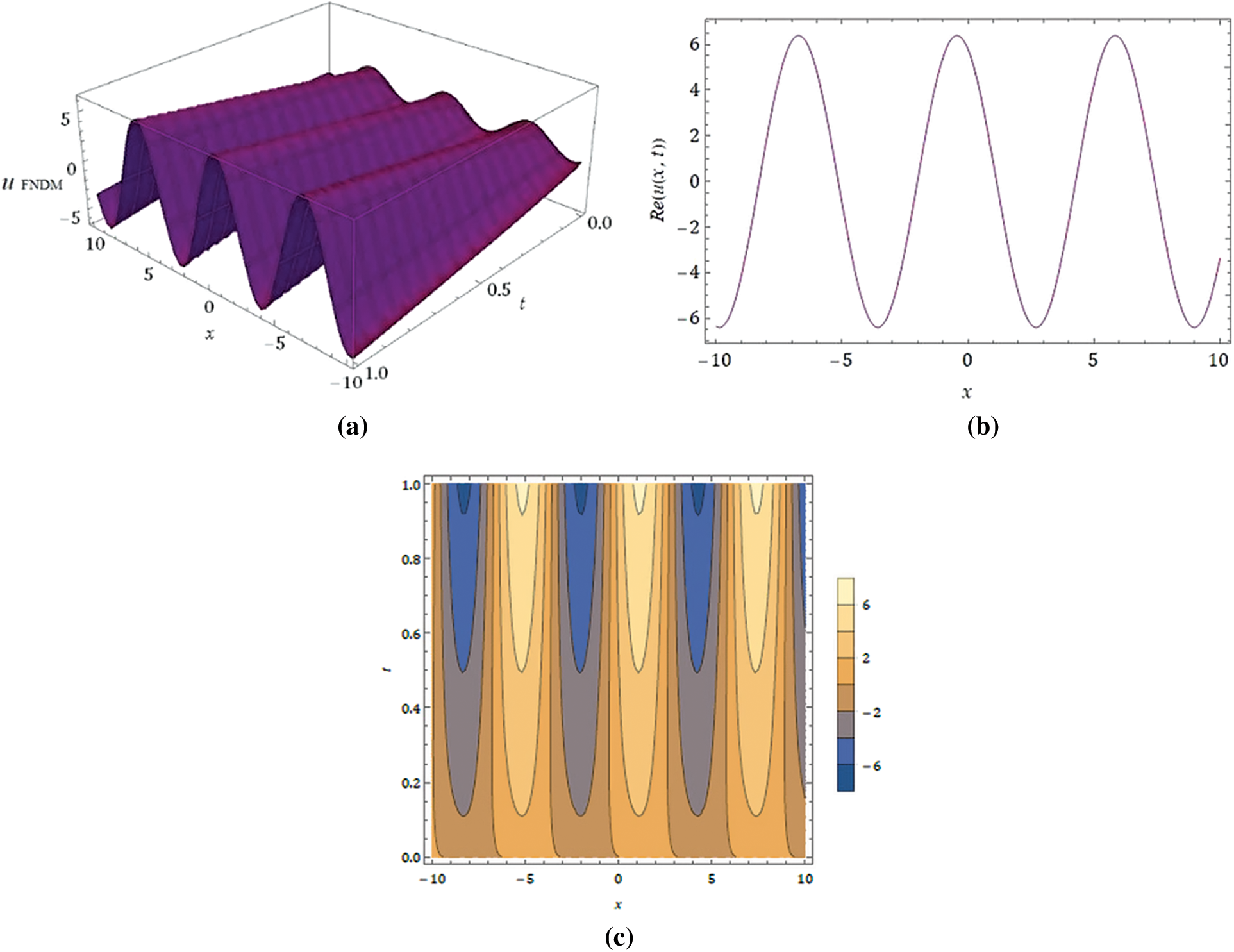
Figure 1: (a) Behaviour for the real part (b) nature of obtained solution at t=1 (c) contour plot for the imaginary part of the FNDM results at α=1.3 and μ=0.5 for the FKE equation

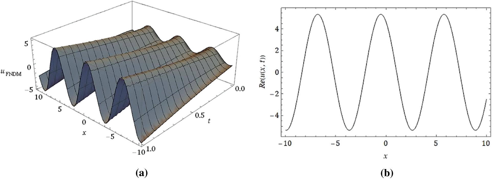
Figure 2: (a) Behaviour for the real part (b) nature of obtained solution at t=1 (c) contour plot for the imaginary part of the FNDM results at α=1.3 and μ=0.75 for the FKE equation

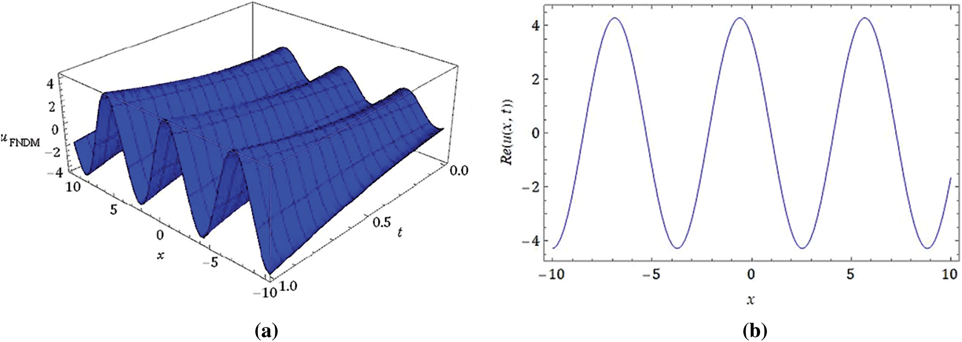
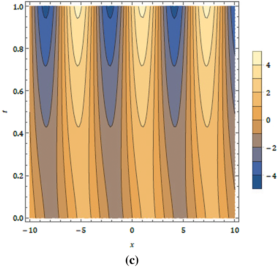
Figure 3: (a) Behaviour for the real part (b) nature of obtained solution at t=1 (c) contour plot for the imaginary part of the FNDM results at α=1.3 and μ=1 for the FKE equation

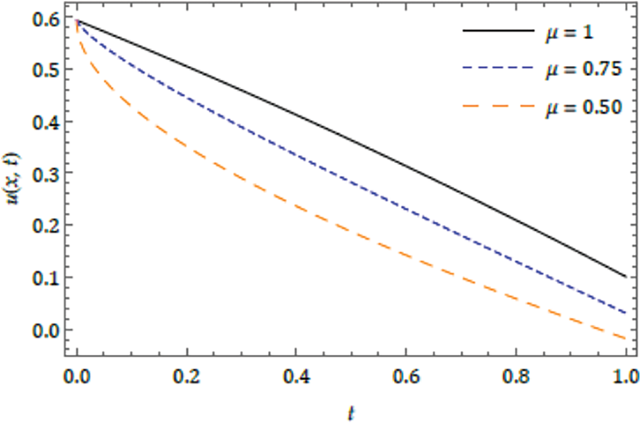
Figure 4: Response of the achieved result for the real part with distinct μ at α=1.3 and x=1 for the FKE equation

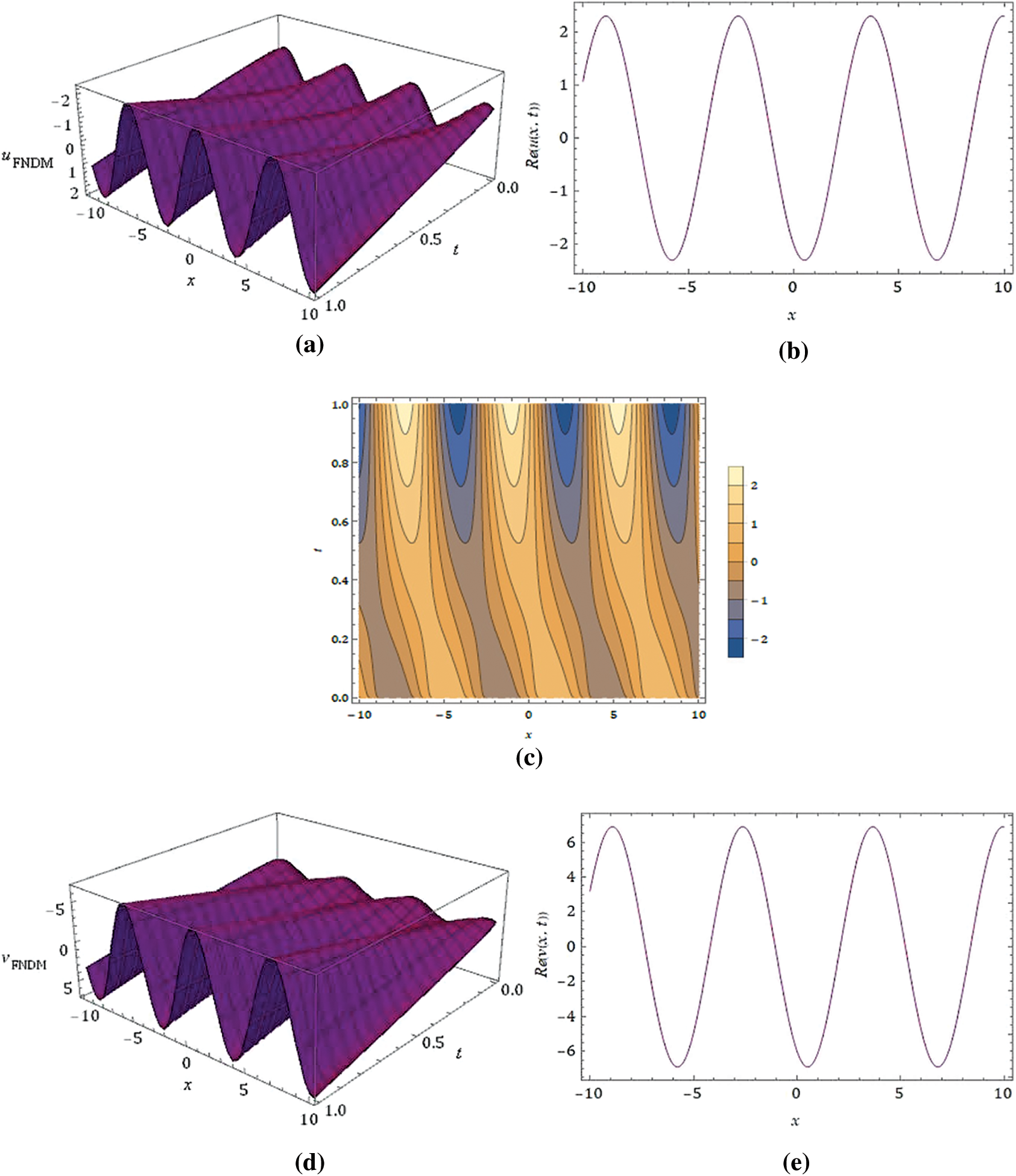
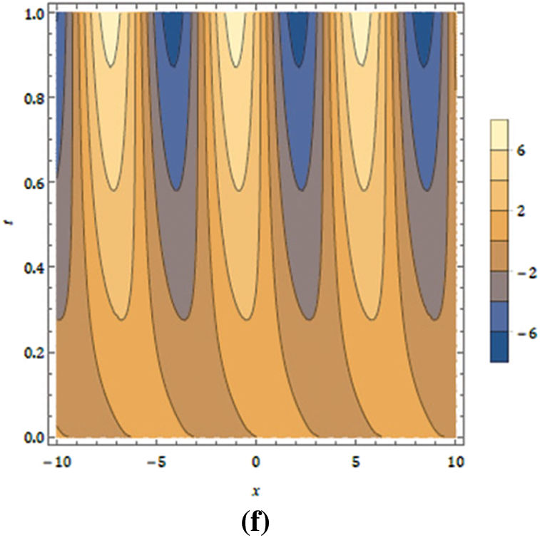
Figure 5: (a) Nature of the real part of u(x,t), (b) response of u(x,t) for the real part at t=1, (c) contour plot of u(x,t), (d) surface of the real part of v(x,t), (e) nature of u(x,t) for the real part at t=1, (f) contour plot of v(x,t) of the obtained solution for the FFMT model at α=1,β=1 and μ=0.5

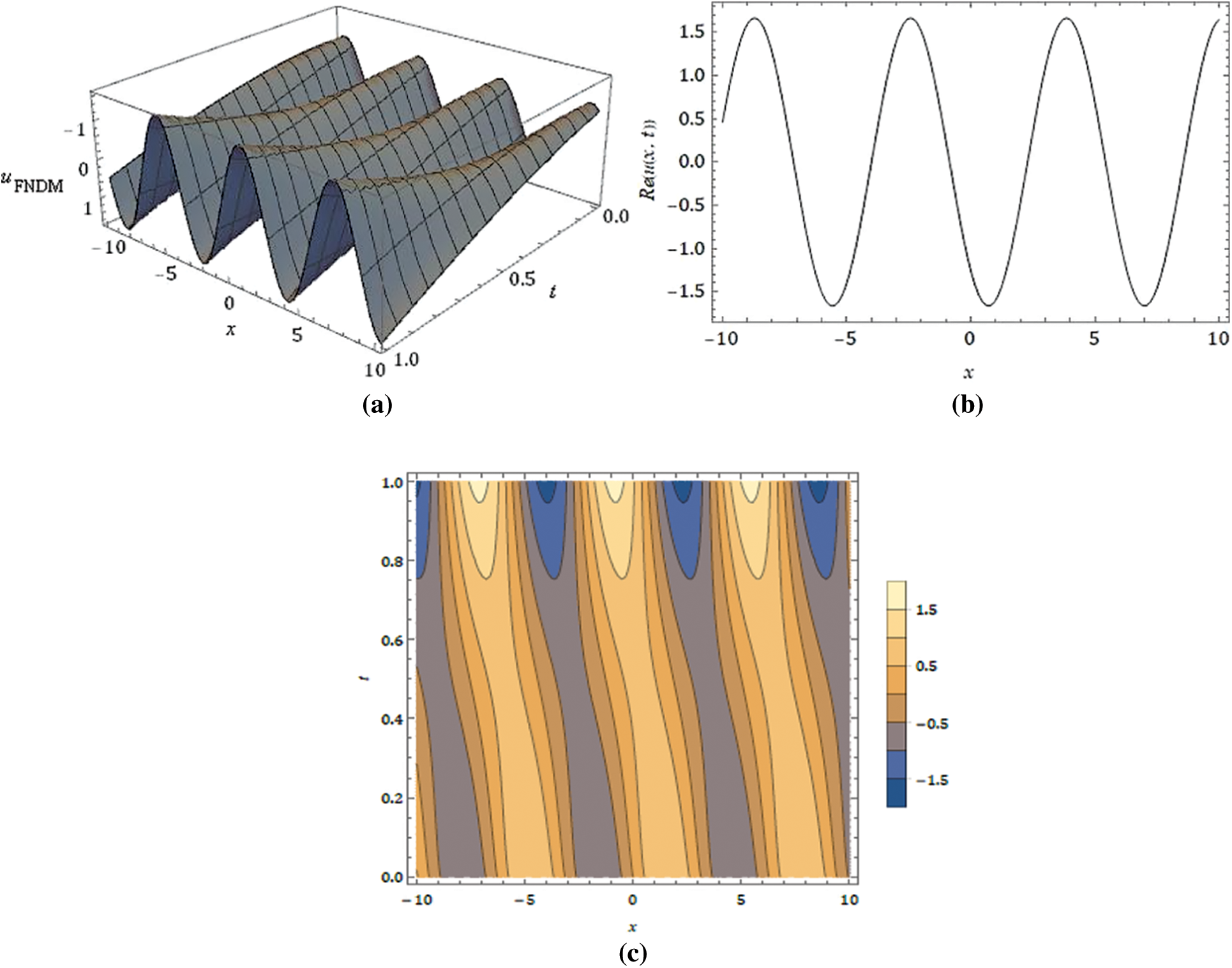
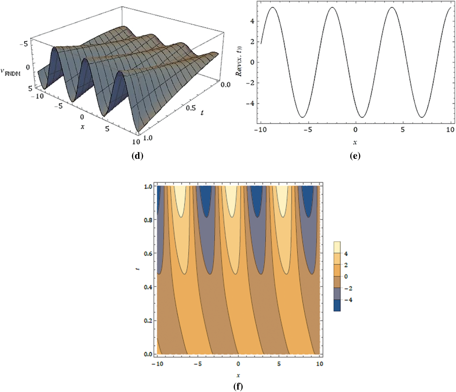
Figure 6: (a) Nature of the real part of u(x,t), (b) response of u(x,t) at t=1, (c) contour plot of u(x,t), (d) surface of the real part of v(x,t), (e) nature of u(x,t) for the real part at t=1, (f) contour plot of v(x,t) of the obtained solution for the FFMT model at α=1,β=1 and μ=0.75

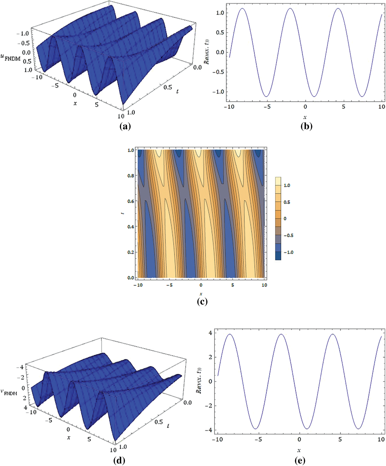
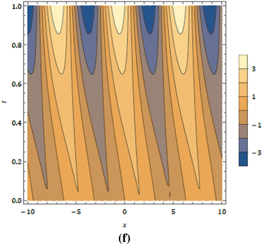
Figure 7: (a) Surface of the real part of u(x,t), (b) response of u(x,t) for the real part at t=1 (c) contour plot of u(x,t), (d) surface of the real part of v(x,t), (e) nature of u(x,t) for the real part at t=1, (f) contour plot of v(x,t) of the obtained solution for the FFMT model at α=1,β=1 and μ=1

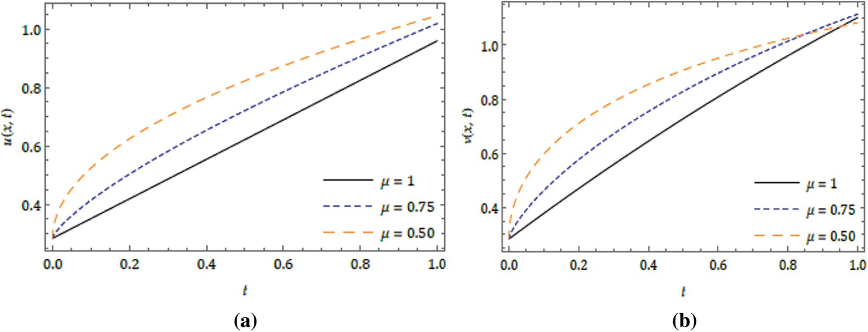
Figure 8: Nature of the real part of (a) u(x,t), (b) v(x,t) with distinct μ at α=1,β=1 and x=5 for the FMT model

6  Conclusion

In this paper, we derived the solution for the projected nonlinear complex system exemplifying the fractional Kundu-Eckhaus equation and the massive Thirring model arising in the quantum field theory with the aid of FNDM. Particularly, counter and coupled surfaces are cited to understand more interesting consequences of the projected system. The novelty of the scheme considered is cleared dissipated to examine coupled systems, and by the projected solution procedure, we can find the solution for nonlinear models associated with complex functions without any dissertation and perturbation. The captured plots show the huge variations with a small change in the order of the system and it can help us to understand more consequences of the projected model. The considered system highly depends on time and analogous consequences with fractional order and it can observe by the present study and further, it can help to diverse classes of coupled nonlinear and complex differential equations. Finally, the results gained by the considered algorithm are interesting as compared to other available results, and hence it can be hired to analyze and examine the various complicated phenomenon.

Funding Statement: The authors received no specific funding for this study.

Conflicts of Interest: The authors declare that they have no conflicts of interest to report regarding the present study.

References

 1.  Liouville, J. (1832). Memoire surquelques questions de geometrieet de mecanique, etsur un nouveau genre de calcul pour resoudreces questions. Journal de l'École Polytechnique, 13, 1–69. [Google Scholar]

 2.  Riemann, G. F. B. (1896). Versucheinerallgemeinen auffassung der integration und differentiation. Leipzig: Gesammelte Mathematische Werke. [Google Scholar]

 3.  Caputo, M. (1969). Elasticita e dissipazione. Bologna: Zanichelli. [Google Scholar]

 4.  Miller, K. S., Ross, B. (1993). An introduction to fractional calculus and fractional differential equations. New York: Wiley. [Google Scholar]

 5.  Podlubny, I. (1999). Fractional differential equations. New York: Academic Press. [Google Scholar]

 6.  Kilbas, A. A., Srivastava, H. M., Trujillo, J. J. (2006). Theory and applications of fractional differential equations, vol. 204. Amsterdam: Elsevier. [Google Scholar]

 7.  Esen, A., Sulaiman, T. A., Bulut, H., Baskonus, H. M. (2018). Optical solitons and other solutions to the conformable space-time fractional Fokas-Lenells equation. Optik, 167(6), 150–156. DOI 10.1016/j.ijleo.2018.04.015. [Google Scholar] [CrossRef]

 8.  Veeresha, P., Yavuz, M., Baishya, C. (2021). A computational approach shallow water forced Korteweg-de Vries equation on critical flow over a hole with three fractional operators. An International Journal of Optimization and Control: Theories & Applications, 11(3), 52–67. DOI 10.11121/ijocta.2021.1177. [Google Scholar] [CrossRef]

 9.  Baleanu, D., Wu, G. C., Zeng, S. D. (2017). Chaos analysis and asymptotic stability of generalized Caputo fractional differential equations. Chaos Solitons Fractals, 102, 99–105. DOI 10.1016/j.chaos.2017.02.007. [Google Scholar] [CrossRef]

10. Veeresha, P., Prakasha, D. G., Baskonus, H. M. (2019). New numerical surfaces to the mathematical model of cancer chemotherapy effect in Caputo fractional derivatives. Chaos, 29(1), 013119. DOI 10.1063/1.5074099. [Google Scholar] [CrossRef]

11. Baskonus, H. M., Sulaiman, T. A., Bulut, H. (2019). On the new wave behavior to the Klein-Gordon-Zakharov equations in plasma physics. Indian Journal of Physics, 93(3), 393–399. DOI 10.1007/s12648-018-1262-9. [Google Scholar] [CrossRef]

12. Veeresha, P., Prakasha, D. G., Kumar, D., Baleanu, D., Singh, J. (2020). An efficient computational technique for fractional model of generalized Hirota-Satsuma-coupled Korteweg-de Vries and coupled modified Korteweg-de Vries equations. Journal of Computational and Nonlinear Dynamics, 15(7), 071003. DOI 10.1115/1.4046898. [Google Scholar] [CrossRef]

13. Baleanu, D., Etemad, S., Rezapour, S. (2020). A hybrid Caputo fractional modeling for thermostat with hybrid boundary value conditions. Boundary Value Problems, 64(1), 64. DOI 10.1186/s13661-020-01361-0. [Google Scholar] [CrossRef]

14. Gao, W., Yel, G., Baskonus, H. M., Cattani, C. (2019). Complex solitons in the conformable (2+1)-dimensional Ablowitz-Kaup-Newell-Segur equation. AIMS Mathematics, 5(1), 507–521. DOI 10.3934/math.2020034. [Google Scholar] [CrossRef]

15. Ghanbari, B., Cattani, C. (2020). On fractional predator and prey models with mutualistic predation including non-local and non-singular kernels. Chaos Solitons & Fractals, 136(2), 109823. DOI 10.1016/j.chaos.2020.109823. [Google Scholar] [CrossRef]

16. Baskonus, H. M., Bulut, H., Sulaiman, T. A. (2019). New complex hyperbolic structures to the Lonngren-wave equation by using sine-Gordon expansion method. Applied Mathematics and Nonlinear Sciences, 4(1), 129–138. DOI 10.2478/AMNS.2019.1.00013. [Google Scholar] [CrossRef]

17. Eskitascıoglu, E. I., Aktaş, M. B., Baskonus, H. M. (2020). New complex and hyperbolic forms for Ablowitz-Kaup-Newell-Segur wave equation with fourth order. Applied Mathematics and Nonlinear Sciences, 4(1), 105–112. DOI 10.2478/AMNS.2019.1.00010. [Google Scholar] [CrossRef]

18. Akinyemi, L., Nisar, K. S., Saleel, C. A., Rezazadeh, H., Veeresha, P. et al. (2021). Novel approach to the analysis of fifth-order weakly nonlocal fractional Schrödinger equation with Caputo derivative. Results in Physics, 31(1), 104958. DOI 10.1016/j.rinp.2021.104958. [Google Scholar] [CrossRef]

19. Veeresha, P., Ilhan, E., Baskonus, H. M. (2021). Fractional approach for analysis of the model describing wind-influenced projectile motion. Physica Scripta, 96(7), 075209. DOI 10.1088/1402-4896/abf868. [Google Scholar] [CrossRef]

20. Baleanu, D., Guvenc, Z. B., Tenreiro Machado, J. A. (2010). New trends in nanotechnology and fractional calculus applications. London, New York: Springer Dordrecht Heidelberg. [Google Scholar]

21. Youssri, Y. H. (2022). Two Fibonacci operational matrix pseudo-spectral schemes for nonlinear fractional Klein-Gordon equation. International Journal of Modern Physics C, 33(4), 2250049. DOI 10.1142/S0129183122500498. [Google Scholar] [CrossRef]

22. Gao, W., Veeresha, P., Cattani, C., Baishya, C., Baskonus, H. M. (2022). Modified predictor-corrector method for the numerical solution of a fractional-order SIR model with 2019-nCoV. Fractal and Fractional, 6(2), 92. DOI 10.3390/fractalfract6020092. [Google Scholar] [CrossRef]

23. Veeresha, P., Baleanu, D. (2021). A unifying computational framework for fractional Gross-Pitaevskii equations. Physica Scripta, 96, 125010. DOI 10.1088/1402-4896/ac28c9. [Google Scholar] [CrossRef]

24. Atta, A. G., Abd-Elhameed, W. M., Moatimid, G. M., Youssri, Y. H. (2021). Shifted fifth-kind Chebyshev Galerkin treatment for linear hyperbolic first-order partial differential equations. Applied Numerical Mathematics, 167(5–6), 237–256. DOI 10.1016/j.apnum.2021.05.010. [Google Scholar] [CrossRef]

25. Baishya, C., Veeresha, P. (2021). Laguerre polynomial-based operational matrix of integration for solving fractional differential equations with non-singular kernel. Proceeding of the Royal Society A, 477(2253), 20210438. DOI 10.1098/rspa.2021.0438. [Google Scholar] [CrossRef]

26. Safare, K. M., Betageri, V. S., Prakasha, D. G., Veeresha, P., Kumar, S. (2021). A mathematical analysis of ongoing outbreak COVID-19 in India through nonsingular derivative. Numerical Methods for Partial Differential Equations, 37(2), 1282–1298. DOI 10.1002/num.22579. [Google Scholar] [CrossRef]

27. Abd-Elhameed, W. M., Youssri, Y. H. (2021). New formulas of the high-order derivatives of fifth-kind Chebyshev polynomials: Spectral solution of the convection–diffusion equation. Numerical Methods for Partial Differential Equations. DOI 10.1002/num.22756. [Google Scholar] [CrossRef]

28. Veeresha, P., Baskonus, H. M., Gao, W. (2021). Strong interacting internal waves in rotating ocean: Novel fractional approach. Axioms, 10(2), 123. DOI 10.3390/axioms10020123. [Google Scholar] [CrossRef]

29. Atta, A. G., Abd-Elhameed, W. M., Youssri, Y. H. (2022). Shifted fifth-kind Chebyshev polynomials Galerkin-based procedure for treating fractional diffusion-wave equation. International Journal of Modern Physics C, 2250102. DOI 10.1142/S0129183122501029. [Google Scholar] [CrossRef]

30. Achar, S. J., Baishya, C., Veeresha, P., Akinyemi, L. (2021). Dynamics of fractional model of biological pest control in tea plants with Beddington-DeAngelis functional response. Fractal and Fractional, 6(1), 1. DOI 10.3390/fractalfract6010001. [Google Scholar] [CrossRef]

31. Kundu, A. (1984). Landau-Lifshitz and higher-order nonlinear systems gauge generated from nonlinear Schrödinger-type equations. Journal of Mathematical Physics, 25(12), 3433–3438. DOI 10.1063/1.526113. [Google Scholar] [CrossRef]

32. Calogero, F., Eckhaus, W. (1987). Nonlinear evolution equations, rescalings, model PDES and their integrability. Inverse Problems, 3(2), 229–262. DOI 10.1088/0266-5611/3/2/008. [Google Scholar] [CrossRef]

33. Eckhaus, W. (1986). The long-time behaviour for perturbed wave-equations and related problems. In: Krödinger, E., Kirchgässner, K. (Eds.Trends in applications of pure mathematics to mechanics. Berlin: Springer. [Google Scholar]

34. Levi, D., Scimiterna, C. (2009). The Kundu-Eckhaus equation and its discretizations. Journal of Physics A, 42(46), 465203–465210. DOI 10.1088/1751-8113/42/46/465203. [Google Scholar] [CrossRef]

35. Aceves, A. B., Wabnitz, S. (1989). Self-induced transparency solitons in nonlinear refractive periodic media. Physics Letters A, 141(2), 37–42. DOI 10.1016/0375-9601(89)90441-6. [Google Scholar] [CrossRef]

36. Eggleton, B. J., de Sterke, C. M.,Slusher, R. E. (1997). Nonlinear pulse propagation in Bragg gratings. Journal of the Optical Society of America B, 14(11), 2980–2993. DOI 10.1364/JOSAB.14.002980. [Google Scholar] [CrossRef]

37. Coleman, S. (1975). Quantum sine-Gordon equation as the massive Thirring model. Physical Review D, 11(8), 2088–2097. DOI 10.1103/PhysRevD.11.2088. [Google Scholar] [CrossRef]

38. Mandelstam, S. (1975). Soliton operators for the quantized sine-Gordon equation. Physical Review D, 11(10), 3026–3030. DOI 10.1103/PhysRevD.11.3026. [Google Scholar] [CrossRef]

39. Arafa, A. A. M., Hagag, A. M. S. (2019). Q-homotopy analysis transform method applied to fractional Kundu-Eckhaus equation and fractional massive Thirring model arising in quantum field theory. Asian-European Journal of Mathematics, 12(1), 1950045. DOI 10.1142/S1793557119500451. [Google Scholar] [CrossRef]

40. Adomian, G. (1984). A new approach to nonlinear partial differential equations. Journal of Mathematical Analysis and Applications, 102(2), 420–434. DOI 10.1016/0022-247X(84)90182-3. [Google Scholar] [CrossRef]

41. Rawashdeh, M. S., Al-Jammal, H. (2016). New approximate solutions to fractional nonlinear systems of partial differential equations using the FNDM. Advances in Difference Equations, 235(1), 1–19. DOI 10.1186/s13662-016-0960-x. [Google Scholar] [CrossRef]

42. Rawashdeh, M. S., Al-Jammal, H. (2016). Numerical solutions for system of nonlinear fractional ordinary differential equations using the FNDM. Mediterranean Journal of Mathematics, 13(6), 4661–4677. DOI 10.1007/s00009-016-0768-7. [Google Scholar] [CrossRef]

43. Rawashdeh, M. S. (2017). The fractional natural decomposition method: Theories and applications. Mathematical Methods in the Applied Sciences, 40(7), 2362–2376. DOI 10.1002/mma.4144. [Google Scholar] [CrossRef]

44. Prakasha, D. G., Veeresha, P., Rawashdeh, M. S. (2019). Numerical solution for (2+1)-dimensional time-fractional coupled Burger equations using fractional natural decomposition method. Mathematical Methods in the Applied Sciences, 42(10), 3409–3427. DOI 10.1002/mma.5533. [Google Scholar] [CrossRef]

45. Veeresha, P., Prakasha, D. G. (2019). Solution for fractional Zakharov-Kuznetsov equations by using two reliable techniques. Chinese Journal of Physics, 60(1), 313–330. DOI 10.1016/j.cjph.2019.05.009. [Google Scholar] [CrossRef]

46. Veeresha, P., Prakasha, D. G., Singh, J. (2019). Solution for fractional forced KdV equation using fractional natural decomposition method. AIMS Mathematics, 5(2), 798–810. DOI 10.3934/math.2020054. [Google Scholar] [CrossRef]

47. Zhao, H., Yuan, J., Zhu, Z. (2017). Integrable semi-discrete Kundu–Eckhaus equation: Darboux transformation, breather, rogue wave and continuous limit theory. Journal of Nonlinear Science, 28(1), 43–68. DOI 10.1007/s00332-017-9399-9. [Google Scholar] [CrossRef]

48. Kumar, D., Manafian, J., Hawlader, F., Ranjbaran, A. (2018). New closed form soliton and other solutions of the Kundu-Eckhaus equation via the extended sinh-Gordon equation expansion method. Optik, 160(6), 159–167. DOI 10.1016/j.ijleo.2018.01.137. [Google Scholar] [CrossRef]

49. Biswas, A., Yildirim, Y., Yasar, E., Triki, H., Alshomrani, A. S. et al. (2018). Optical soliton perturbation with full nonlinearity for Kundu-Eckhaus equation by modified simple equation method. Optik, 157(22), 1376–1380. DOI 10.1016/j.ijleo.2017.12.108. [Google Scholar] [CrossRef]

50. Biswas, A., Ekici, M., Sonmezoglu, A., Zhou, Q., Moshokoa, S. P. et al. (2018). Optical soliton perturbation with full nonlinearity for Kundu-Eckhaus equation by extended trial function scheme. Optik, 160(22), 17–23. DOI 10.1016/j.ijleo.2018.01.111. [Google Scholar] [CrossRef]

51. Guo, L., Wang, L., Cheng, Y., He, J. (2017). High-order rogue wave solutions of the classical massive Thirring model equations. Communications in Nonlinear Science and Numerical Simulation, 52, 11–23. DOI 10.1016/j.cnsns.2017.04.010. [Google Scholar] [CrossRef]

52. Xie, X., Tian, B., Sun, W., Sun, Y. (2015). Rogue-wave solutions for the Kundu-Eckhaus equation with variable coefficients in an optical fiber. Nonlinear Dynamics, 81(3), 1349–1354. DOI 10.1007/s11071-015-2073-6. [Google Scholar] [CrossRef]

53. Xie, X., Yan, Z. (2018). Soliton collisions for the Kundu-Eckhaus equation with variable coefficients in an optical fiber. Applied Mathematics Letters, 80, 48–53. DOI 10.1016/j.aml.2018.01.003. [Google Scholar] [CrossRef]

54. Manafian, J., Lakestani, M. (2016). Abundant soliton solutions for the Kundu-Eckhaus equation via tan(ϕ(ξ))-expansion method. Optik, 127(14), 5543–5551. DOI 10.1016/j.ijleo.2016.03.041. [Google Scholar] [CrossRef]

55. Baskonus, H. M., Bulut, H. (2015). On the complex structures of Kundu-Eckhaus equation via improved Bernoulli sub-equation function method. Waves Random Complex Media, 25(4), 720–728. DOI 10.1080/17455030.2015.1080392. [Google Scholar] [CrossRef]

56. Mittag-Leffler, G. M. (1903). Sur la nouvelle function Eα(x). Comptes Rendus de l'Académie des Sciences, 137, 554–558. [Google Scholar]

57. Khan, Z. H., Khan, W. A. (2008). N-transform properties and applications. NUST Journal of Engineering Sciences, 1(1), 127–133. DOI 10.24949/njes.v1i1.69. [Google Scholar] [CrossRef]

58. Loonker, D., Banerji, P. K. (2013). Solution of fractional ordinary differential equations by natural transform. International Journal of Engineering Science, 12(2), 1–7. [Google Scholar]

This work is licensed under a Creative Commons Attribution 4.0 International License, which permits unrestricted use, distribution, and reproduction in any medium, provided the original work is properly cited.