Computer Modeling in Engineering & Sciences

---

DOI: 10.32604/cmes.2022.022210

ARTICLE

Static Analysis of Doubly-Curved Shell Structures of Smart Materials and Arbitrary Shape Subjected to General Loads Employing Higher Order Theories and Generalized Differential Quadrature Method

Francesco Tornabene*, Matteo Viscoti and Rossana Dimitri

Department of Innovation Engineering, School of Engineering, University of Salento, Lecce, 73100, Italy
*Corresponding Author: Francesco Tornabene. Email: francesco.tornabene@unisalento.it
Received: 28 February 2022; Accepted: 11 May 2022

1  Introduction

New advances in many engineering applications are based on the employment of smart innovative materials and appliances characterized by non-conventional shapes [1,2]. Very complex mechanical properties are very frequently required, together with an increased need for lightweight materials [3]. As a matter of fact, when unconventional materials and geometries are adopted, the structural behaviour is not easy to be predicted a priori with simple but effective models due to the absence of symmetry planes [4,5].

In this perspective, laminated structures are widespread solutions for achieving unconventional and optimized structural performances. As it is well-known, classical composite materials usually induce an orthotropic behaviour of the overall structure [6]. Nevertheless, new solutions can be found in literature where very complex deformation mechanisms can be induced, together with coupling effects. Moreover, several engineering manufacturing processes employ architectured geometries that have been conceived for the fulfillment of different aesthetic, ergonomic, and aerodynamic requirements [7]. An important reason comes from the endeavor to obtain the best form under fixed load cases and external constraints layup [8]. In fact, an effective reduction of the material is sought in this way. All shell structures are spatially distributed volumes [9,10]. For this reason, advanced design skills are required for a correct mathematical modelling of their shape and material properties. Moreover, the accuracy of a correct modelling is crucial for its reliability since the presence of curvature significantly orients the structural behaviour, as well as the constitutive relationships [11].

As a matter of fact, three-dimensional (3D) solid simulations based on the widespread Finite Element Method (FEM) are nowadays the most adopted strategy for the structural assessment of curved and layered shells [12,13]. Accordingly, such models lead to a very demanding computational cost for the simulation [14]. For this reason, two-dimensional (2D) alternative approaches have been derived. The most famous strategy is Equivalent Single Layer (ESL) [15–17], which assesses the entire structural problem on a reference surface whose generic point is located in the middle thickness of the solid. In particular, in reference [16] an extensive study with higher order theories for doubly-curved shell structures is provided, and in reference [17] an ESL higher order model is developed for laminated composite curved structures. In the same way, the Layer-Wise (LW) approach [18–22] introduces a 2-manifold for each layer of the stacking sequence. In reference [19] the dynamic behaviour of anisotropic doubly-curved shells is investigated with a higher order LW approach, whereas in reference [20] an equivalent LW model is developed, accounting for an efficient description of the kinematic field, referring to the intrados and extrados of the structure. In the so-called Sub-Laminate Theory (SLT) a series of reference surfaces are defined for a specific group of the entire lamination scheme [23–25]. For the LW and the SLT, the compatibility conditions between the various reference surfaces are taken into account during the global matrices assembly. Generally speaking, LW provides more accurate results than the ESL approach, but it can be very high computationally demanding since the overall number of Degrees of Freedom (DOFs) comes to be proportional to the layers within the laminate [26]. Within the ESL framework, the number of unknown variables is not dependent on the actual stacking sequence. Moreover, suppose a higher order set of axiomatic assumptions is included in the model. In that case, the accuracy of ESL 2D formulations can be compared to that of the 3D FEM and LW solutions even for generally anisotropic lamination schemes [27].

As it is well known, classical finite element simulations are characterized by a local pre-determined polynomial approximation of the unknown field variable between two adjacent points. On the other hand, when shell elements with curvatures are considered, some issues like the shear locking can emerge, thus invalidating the simulation [28,29]. For this reason, very refined meshes are implemented so that very accurate results are requested. In this way, the geometric and simulation discretization error is reduced, but the computational cost increases a lot.

In contrast, the IsoGeometric Approach (IGA) accounts for the employment of the actual geometry of the structure directly taken from the Computer Aided Design (CAD) process in the theoretical modelling [30–34]. As a consequence, arbitrary interpolating functions are developed. Throughout literature, IGA has been employed for both the strong and weak implementations of disparate structural problems with curved edges and shapes. In particular, in reference [34] the IGA approach has been adopted for the buckling analysis of 3D plates, taking into account 2D computation of Non-Uniform Rational B-Spline (NURBS) curves, as well as the enforcement of boundary conditions. Furthermore, the hybrid meshfree collocation method is employed in reference [35], and a computationally efficient formulation is obtained, which is characterized by the advantages of IGA and meshfree methods.

When laminated doubly-curved shells are investigated by means of 2D models, a key aspect is the parametrization of the reference surfaces. It is feasible that a set of principal curvilinear coordinates are provided starting from the geometric properties of the structure. In the case of shells of arbitrary shape, a distortion algorithm is proposed so that the physical domain is described with a rectangular computational interval. To this end a set of generalized blending functions are developed [36,37]. They are based on the geometric description of the shell edges and the location of the corners of the structure within the physical domain. When IGA methodology is followed, NURBS curves are employed for this task. In references [38,39], an interesting insight into the computation of such curves is provided.

Within the ESL 2D simulations, since the 3D shell structure is reduced to its equivalent reference surface as described in references [40,41] the three-dimensional unknown field variable should be expressed in terms of a set of predetermined through-the-thickness shape functions [42–45], each of them arranged employing a generalized matrix formulation [46,47]. Accordingly, reference [42] employs power polynomials for the assessment of all thickness functions set and derives a closed-form analytical solution, whereas in references [43,44] a higher order power assumption is adopted only for in-plane displacement components. As far as ESL theories is concerned, both polynomial and trigonometric functions can be adopted along each shell principal direction [48–50]. As the order of the kinematic expansion increases, the so-called Higher Order Shear Deformation Theories (HSDTs) come out [16]. The above-mentioned generalized approach also embeds classical theories like the First Order Shear Deformation Theory (FSDT) [51,52] and the Third Order Shear Deformation Theory (TSDT) [53–55] which considers a first and a third-order polynomial expansion for the in-plane kinematic field, respectively. The out-of-plane direction is characterized by a constant distribution of the displacement field instead, thus neglecting any kind of stretching and shear effect. The employment of non-uniform through-the-thickness assumptions is crucial for modelling the actual deflection of the structure. Actually, in reference [56] it is shown that the out-of-plane stretching plays an important role in the deformation response, whereas in reference [57] the shear contribution in the total deflection of composite laminated structure is outlined. Even though an axiomatic selection of thickness functions can be assessed, some refined theories have been derived for orthotropic laminated structures in which the through-the-thickness hypotheses are based on the mechanical characteristics of the constituent materials [58–61]. In particular, in reference [58] the classical FSDT theory is refined with the introduction of a shear thickness function derived from the actual lamination scheme of the selected plate. Furthermore, in reference [59] the same approach has been applied to mono-dimensional (1D) beams. In the case of laminated shells the unknown field variable dispersion should fulfil the interlaminar continuity since a piecewise transverse displacement field and shear stress distribution should be modelled. Moreover, it is feasible that the shear effect is embedded in the formulation, since experimental tests show that its contribution turns out to be prominent in laminated structures [62,63]. For this reason, the LW approach is the most suitable strategy. On the other hand, the ESL approach can provide good results too if the so-called zigzag functions are adopted for the field variable description. In reference [64] an interesting review for multilayered theories is reported, where the selection of thickness functions accounts for continuous transverse stresses and a discontinuous first order derivative of the same quantities for both in-plane and out-of-plane components. In references [65,66] instead, a discontinuous first order derivative of the in-plane displacement components is provided in an effective way from the introduction of a piecewise function at the first order of the kinematic expansion.

Some considerations should be made on the treatment of external surface loads distributions within a 2D formulation. Classical solutions for plate problems [67,68] account in general for a mere computation of normal external loads within the equilibrium equations. In the case of higher order assumptions on the displacement field variable, the external loads should be inserted within the 2D approach. An effective procedure for the assessment of external loads is based on the Static Equivalence Principle [16,69]. The same methodology can be applied to classical refined models when a higher order displacement field assumption is taken along each in-plane field variable. Throughout literature, a huge variety of works can be found where the static performance of plates and shells is evaluated under a uniform distribution of normal and tangential loads [70–75]. In reference [75] a consistent method is proposed for concentrated loads within an ESL model directly in a strong form. In particular, a smooth continuous function is taken into account, and the calibration of the shape and position parameters can lead to a proper modelling of the singularity induced by point and line loads. On the other hand, there are only few works from literature dealing with a general distribution of surface pressure. A different group of studies investigates the problem of concentrated and line loads, starting from the numerical approximation methods of the Delta-Dirac function. Among others, the interested reader can refer to the articles by Eftekhari et al. [76–78], where the Dirac-Delta function is discretized with success taking into account the employed numerical method. In particular, in reference [76] moving concentrated loads have been applied to 1D structures starting from the definition of the Dirac-Delta function. Then, in reference [77] the formulation has been extended to 2D structural problems. Moving load problems have been treated in reference [78] with the well-known Heaviside function. Generally speaking, the approximating function of a singularity problem should fulfill some characteristic properties derived from the theoretical definition of concentrated loads; otherwise, it should be properly normalized. These kinds of pressures are singularities in a differential continuum model, such that various numerical techniques have been proposed for their approximation with smooth functions [79–81]. According to the author’s knowledge, there are some works accounting for a Gaussian distribution (see reference [82] among others). An interesting problem related to concentrated loads on curved structures is the so-called pinched cylinder. In references [83–85] a series of theoretical developments have been provided for a circular cylinder subjected to a point load applied at the diameter of the surface.

As far as the numerical implementation is concerned, several articles can be found in which spectral collocation methods are adopted within IGA framework. Among them, the Generalized Differential Quadrature (GDQ) method [86–90] has demonstrated to be a reliable tool since it overcomes many computational drawbacks. Based on polynomial functional approximation methods, the GDQ has been successfully applied to a series of structural problems [91,92]. In particular, some works can be found where GDQ has been adopted for the dynamic analysis of smart structures, as well as multifield problems [93,94]. It has been shown that it is an extension of pseudospectral collocation methods since the similar levels of accuracy are obtained when the same computational grid is adopted [95–97]. On the other hand, the generalized procedure for the calculation of weighting coefficients based on Lagrange polynomials for the global interpolation is not based on the actual selection of discrete points and the derivation order. In particular, the GDQ method provides the best performance among all the numerical techniques belonging to the weighted residual class. In reference [98] the outcomes of the free vibration analysis of thin-walled beams calculated by means of the GDQ method are compared to those coming from a 1D Ritz formulation. Other works [99–102] provide the theoretical assessment together with some parametric static and dynamic analyses of shells of different curvatures characterized by innovative material like Carbon Nanotubes (CNTs) and Functionally Graded Materials (FGMs). In reference [103] FGM structures have been investigated by employing a semi-analytical model. In reference [104] an effective homogenization algorithm is developed for the mechanical assessment of sandwich shells with both honeycomb and re-entrant patterns. Referring to pantographic lattice structures, the widespread method for the computation of equivalent elastic properties is the well-known Neumann’s principle [105], accounting for the computation of generalized stiffnesses starting from simple independent load cases [106–108]. The accuracy of the solution lies in the theoretical hypothesis considered for the numerical modelling. In particular, some considerations should be made on the nodal area within the honeycomb cell, as well as the bending and shear effects of vertical and inclined struts [109–111].

Once the 2D solution is provided on the reference surface of a doubly-curved shell, the post-processing algorithm is crucial for the reconstruction of both static and kinematic quantities along the three-dimensional solid. Actually, both the ESL and the LW formulation account for the assessment of the generalized unknown field variables lying on the reference surface. Accordingly, in the case of simulations performed with the FEM, the solution is calculated at the discrete set of nodes of the computational grid. Then, a reconstruction along the continuum domain should be assessed. Referring to the latter, there are three main classes of methodologies for the solution extrapolation, namely the Superconvergent Patch Recovery (SPR) [112,113], the Averaging Method (AVG) [114,115] and the Projection Method (PROJ) [116]. As far as the through-the thickness equilibrium-based recovery procedure is concerned, the generalized constitutive relationship can be adopted as usual, but a correction of shear and membrane stresses is essential so the boundary conditions related to applied loads can be fulfilled [117–120].

In the present work, an ESL theoretical formulation is proposed for generally anisotropic doubly-curved shells of arbitrary shapes by means of the ESL method. The reference surface of the structure is described employing the main outcomes of differential geometry, setting an orthogonal curvilinear set of principal coordinates. A NURBS based generalized set of blending functions is employed for the distortion of the physical domain in the case of arbitrarily-shaped structures. The displacement field component vector is intended to be the unknown variable of the problem, and it is expressed via the employment of a generalized set of thickness functions. Actually, a higher order kinematic expansion is performed together with a consistent zigzag function to properly catch all the possible stretching and warping effects within each layer, as well as coupling issues at the interlaminar stage. A generalized weak expression of the field variable is introduced, accounting for higher order shape functions for the interpolation alongside the reference surface [121]. A general distribution of surface loads has been considered in the model, setting a Gaussian and a Super-Elliptic distribution for the application of external loads along each principal direction of the shell. In particular, the calibration of distribution parameters leads to model different load cases. The fundamental governing equations, derived from the Minimum Potential Energy Principle, are numerically tackled by the GDQ method. The Generalized Integral Quadrature (GIQ) method has been adopted for the computation of integrals [16]. The GIQ moves from the above-discussed GDQ procedure, and it allows performing numerical integrations following an effective quadrature approach.

The theoretical formulation proposed in this manuscript has been implemented in the DiQuMASPAB software [122], a research code based on the GDQ method accounting for static and dynamic simulations on doubly-curved shell structures. All the numerical examples of mechanical properties have been included in the built-in material library. The graphic user interface provided by the software allows to implement the lamination scheme, the geometry of the structure, as well as external load and boundary conditions features. The structures that are considered for the numerical validation account for different mechanical issues, namely the presence of a single and double curvature, the number of layers and the presence of the soft core. Different loading conditions have been adopted. The equilibrium-based 3D reconstruction of mechanical quantities has been demonstrated to be very efficient in accordance with the predictions of refined 2D and 3D solutions. The same level of accuracy has been outlined in the case of lamination schemes with a lattice layer characterized by a macro mechanical orthotropic behaviour. Any performance reduction has been observed when a mapping of the physical domain has been required.

2  Geometrical Description of a Doubly-Curved Shell

According to the ESL formulation, a doubly-curved shell should be referred to its reference surface whose points are located at the middle thickness of the structure. It should be remarked that a generic three-dimensional solid can be expressed with respect to a Cartesian global reference system Ox1x2x3 of unit vectors e1,e2,e3 in terms of three parameters α1,α2,α3:

R(α1,α2,α3)=f1(α1,α2,α3)e1+f2(α1,α2,α3)e2+f3(α1,α2,α3)e3(1)

being R(α1,α2,α3) the three-dimensional position vector, and fi(α1,α2,α3) for i=1,2,3 a continuous function. If the variables α1,α2,α3 are taken as a set of curvilinear coordinates, it is possible to introduce the above discussed reference surface r(α1,α2) starting from Eq. (1) as follows [16]:

R(α1,α2,ζ)=r(α1,α2)+ζn(α1,α2)(2)

where the α3=ζ has been selected alongside the normal direction of r. A schematic representation of the ESL assessment of the shell geometry has been reported in Fig. 1. The normal unit vector can be computed if the partial derivatives of r(α1,α2) with respect to αi=α1,α2, namely r,i=∂r/∂r∂αi∂αi, are known:

n=r,1×r,2|r,1×r,2|(3)

More specifically, Eq. (2) describes a doubly-curved shell when all the variables vary in a closed interval. In particular, it should be stated that R(α1,α2,ζ)∈[α10,α10]×[α20,α21]×[−h/h22,h/h22]. Accordingly, shell thickness h(α1,α2) can be defined starting from Eq. (2), according to the following expression taken from reference [16]:

h(α1,α2)=∑k=1lhk(α1,α2)=∑k=1l(ζk+1(α1,α2)−ζk(α1,α2))(4)

where hk(α1,α2)=ζk+1(α1,α2)−ζk(α1,α2) is the width of the k-th lamina of the stacking sequence composed of l∈N layers located within the interval [ζk,ζk+1]⊆[−h/h22,h/h22]. If the second order derivatives r,ij=∂2r/∂2r(∂αi∂αj)(∂αi∂αj) of the reference surface with αi,αj=α1,α2 are calculated, it is possible to compute the principal radii of curvature Ri=R1,R2 in each point of the physical domain:

Ri=−r,i⋅r,ir,ii⋅nfori=1,2(5)

In addition, the well-known Lamè parameters Ai=A1,A2 are defined as follows:

Ai=r,i⋅r,ifori=1,2(6)

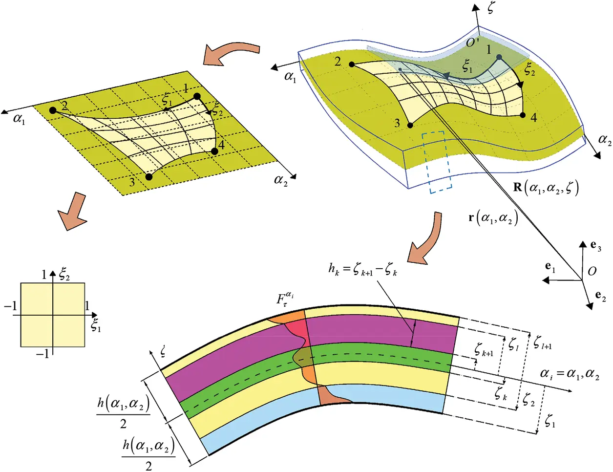
Figure 1: Graphic representation of the ESL methodology for the structural assessment of doubly-curved shells of arbitrary shape. NURBS mapping of the structure and definition of a 2D rectangular computational domain

Starting from Eqs. (1) and (2), the parameters Hi(α1,α2,ζ) are defined, accounting for the curvature effect alongside the thickness direction ζ:

Hi(α1,α2,ζ)=1+ζRi(α1,α2)fori=1,2(7)

Accordingly, in the case of straight shells along the αi principal direction, Eq. (7) turns into Hi(α1,α2,ζ)=1.

In the present manuscript, doubly-curved shells of variable thickness [16] have been considered; therefore, a generalized analytical expression of h=h(α1,α2) is provided hereafter:

hk(α1,α2)=hk0h~(α1,α2)=hk0(1+∑j4δjϕj(α1,α2)+δ¯)(8)

being hk0 the reference height of the k-th layer and δj for j=1,…,4 a scaling parameter, whereas δ¯ is a constant dimensionless shift number. In Eq. (8), thickness variation h~(α1,α2) has been described in terms of four analytical expressions ϕj(α1,α2) employing a dimensionless coordinate defined along each αi=α1,α2 principal direction of the shell, according to the following equation:

α¯i=αi−αi0αi1−αi0fori=1,2(9)

In the present formulation, the expressions of ϕj(α1,α2) for j=1,…,4 have been implemented, being αjm∈[0,1], nj∈N and pj∈R [16]:

ϕj(α1,α2)={α¯ipje−(α¯iαjm)pj(sin⁡(π(njα¯i+αjm)))p1fori=1,2j=1,2ϕj(α1,α2)={(1−α¯i)pje−(1−α¯iαjm)pj(sin⁡(π(nj(1−α¯i)+αjm)))pjfori=1,2j=3,4(10)

When an arbitrary curve is considered lying on the reference surface r(α1,α2) described with principal coordinates, a local reference system composed of three unit vectors nn, ns and nζ should be defined in each point of the curve at issue. More specifically, ns accounts for the tangential unit vector of the curve, whereas nn is the normal unit vector of the curve. nζ denotes the bi-normal direction. Referring to O′α1α2ζ middle surface reference system, nn, ns and nζ components can be computed in each point of the curve, leading to:

n n = [ n n1 ​​  n n2   n n3 ] T n s = [ n s1   n s2  n s3 ] T n ζ = [ n ζ1   n ζ1   n ζ2  ] T (11)

Since the curve at issue lies on r(α1,α2), it should be noted that nn3=ns3=nζ1=nζ2=0 and nζ3=1.

3  NURBS Blending of the Physical Domain

In the previous paragraph, the geometry of a generic doubly-curved shell has been described starting from the reference surface r(α1,α2), according to the ESL framework. Nevertheless, it is possible to perform a distortion of the original physical domain [α10,α11]×[α20,α21] in order to take into account structures of arbitrary shape. To this purpose, a set of blending coordinates ξ1,ξ2∈[−1,1] are introduced along the parametric lines of the mapped shell, as it has been shown in Fig. 1. In particular, the four edges of the physical are identified on the physical domain according to the following nomenclature [16]:

West edge(W)→ξ2=−1→(α1,α2)=(α¯1(1)(ξ1),α¯2(1)(ξ1))South edge(S)→ξ1=1→(α1,α2)=(α¯1(2)(ξ2),α¯2(2)(ξ2))East edge(E)→ξ2=1→(α1,α2)=(α¯1(3)(ξ1),α¯2(3)(ξ1))North edge(N)→ξ1=−1→(α1,α2)=(α¯1(4)(ξ2),α¯2(4)(ξ2))(12)

In Eq. (12), the symbols α¯i(j) with i=1,2 and j=1,…,4 account for the parametric representation of the outer sides of the reference surface alongside the physical domain, collected in the vectors α¯i=[α¯i(1)(ξ1)α¯i(2)(ξ2)α¯i(3)(ξ1)α¯i(4)(ξ2)]T for i=1,2. In the same way, the four corners of r(α1,α2) denoted with (α1(j),α2(j)) for j=1,…,4 are arranged so that αi=[αi(1)αi(2)αi(3)αi(4)]T with i=1,2. Based on these definitions, it is possible to assess the blending expressions αi(ξ1,ξ2) of the physical domain according to the following matrix-form expressions:

[α1(ξ1,ξ2)α2(ξ1,ξ2)]=[b¯00b¯][B¯00B¯][α~1α~2](13)

being α~i=[α¯iαi]T for i=1,2. Accordingly, the following definitions for b¯ and B¯ should be assessed:

b¯=[bb],B¯=[12I00−14B](14)

where I is the identity matrix. On the other hand, vectors b and matrix B read as follows:

b=[(1−ξ2)(1+ξ1)(1+ξ2)(1−ξ1)]B=[(1−ξ1)0000(1−ξ2)0000(1+ξ1)0000(1+ξ2)](15)

Starting from Eq. (13), it is possible to derive an expression for partial derivatives with respect to in-plane directions α1,α2 in terms of natural coordinates ξ1,ξ2 thanks to the well-known chain rule [16]:

[∂∂α1∂∂α2]=[∂ξ1∂α1∂ξ2∂α1∂ξ1∂α2∂ξ2∂α2][∂∂ξ1∂∂ξ2]=[ξ1,α1ξ2,α1ξ1,α2ξ2,α2][∂∂ξ1∂∂ξ2](16)

where the definitions ξi,αj=∂ξi/∂ξi∂αj∂αj for i,j=1,2 are introduced. In the case of arbitrarily-shaped physical domains, it is very likely that the partial derivatives with respect to ξ1,ξ2 should be referred to the principal coordinate system as well. For this reason, the following transformation should be declared, setting J the Jacobian matrix of Eq. (13):

[∂∂ξ1∂∂ξ2]=[∂α1∂ξ1∂α2∂ξ1∂α1∂ξ2∂α2∂ξ2][∂∂α1∂∂α2]=J[∂∂α1∂∂α2](17)

If det(J)≠0, the inverse form J−1 of the Jacobian matrix occurring in Eq. (17) can be calculated, thus obtaining:

J−1=1det(J)[∂α2∂ξ2−∂α2∂ξ1−∂α1∂ξ2∂α1∂ξ1](18)

Accordingly, the inverse relation of Eq. (17) accounts as follows:

[∂∂α1∂∂α2]=J−1[∂∂ξ1∂∂ξ2]=[∂ξ1∂α1∂ξ2∂α1∂ξ1∂α2∂ξ2∂α2][∂∂ξ1∂∂ξ2](19)

From a direct comparison between Eqs. (16) and (19), the definition of coefficients ξi,αj can be assessed [16]:

ξ1,α1=∂ξ1∂α1=1det(J)∂α2∂ξ2,ξ1,α2=∂ξ1∂α2=−1det(J)∂α1∂ξ2ξ2,α1=∂ξ2∂α1=−1det(J)∂α2∂ξ1,ξ2,α2=∂ξ2∂α2=1det(J)∂α1∂ξ1(20)

For the sake of completeness, first order partial derivatives det(Jξi) with i=1,2 of det(J) with respect to natural coordinates ξ1,ξ2 can be expressed as:

det(Jξ1)=∂α1∂ξ1∂2α2∂ξ1∂ξ2−∂α2∂ξ1∂2α1∂ξ1∂ξ2+∂α2∂ξ2∂2α1∂ξ12−∂α1∂ξ2∂2α2∂ξ12det(Jξ2)=−∂α1∂ξ2∂2α2∂ξ1∂ξ2+∂α2∂ξ2∂2α1∂ξ1∂ξ2−∂α2∂ξ1∂2α1∂ξ22+∂α1∂ξ1∂2α2∂ξ22(21)

Following a similar procedure of that adopted in Eqs. (16)–(20), the chain rule can also be employed for the computation of second order derivatives with respect to α1,α2 principal coordinates in terms of ∂/∂∂ξ1∂ξ1 and ∂/∂∂ξ2∂ξ2. The final expression for second order mixed derivatives looks as follows [16]:

∂2∂α1∂α2=ξ1,α1ξ1,α2∂2∂ξ12+ξ2,α1ξ2,α2∂2∂ξ22+(ξ1,α1ξ2,α2+ξ1,α2ξ2,α1)∂2∂ξ1∂ξ2+ξ1,α1α2∂∂ξ1+ξ2,α1α2∂∂ξ2(22)

being ξj,α1α2 with j=1,2 a transformation coefficient reading as:

ξ1,α1α2=1det(J)2(−∂α2∂ξ2∂2α1∂ξ1∂ξ2+∂α2∂ξ2∂α1∂ξ2det(Jξ1)det(J)+∂α2∂ξ1∂2α1∂ξ22−∂α2∂ξ1∂α1∂ξ2det(Jξ2)det(J))ξ2,α1α2=1det(J)2(−∂α2∂ξ1∂2α1∂ξ1∂ξ2+∂α1∂ξ2∂α1∂ξ1det(Jξ1)det(J)+∂α2∂ξ2∂2α1∂ξ12−∂α2∂ξ1∂α1∂ξ1det(Jξ2)det(J))(23)

In addition, one gets the following expression for pure second order derivatives with respect to αi direction, setting i=1,2 [16]:

∂2∂αi2=ξ1,αi2∂2∂ξ12+ξ2,αi2∂2∂ξ22+2ξ1,αiξ2,αi∂2∂ξ1∂ξ2+ξ1,αiαi∂∂ξ1+ξ2,αiαi∂∂ξ2fori=1,2(24)

where the coefficients ξj,αiαi for i,j=1,2 complete expression are thus reported:

ξ1,α1α1=1det(J)2(∂α2∂ξ2∂2α2∂ξ1∂ξ2−(∂α2∂ξ2)2det(Jξ1)det(J)−∂α2∂ξ1∂2α2∂ξ22+∂α2∂ξ1∂α2∂ξ2det(Jξ2)det(J))ξ1,α2α2=1det(J)2(∂α1∂ξ2∂2α1∂ξ1∂ξ2−(∂α1∂ξ2)2det(Jξ1)det(J)−∂α1∂ξ1∂2α1∂ξ22+∂α1∂ξ1∂α1∂ξ2det(Jξ2)det(J))ξ2,α1α1=1det(J)2(−∂α2∂ξ2∂2α2∂ξ12+∂α2∂ξ2∂α2∂ξ1det(Jξ1)det(J)+∂α2∂ξ1∂2α2∂ξ1∂ξ2−(∂α2∂ξ1)2det(Jξ2)det(J))ξ2,α2α2=1det(J)2(−∂α1∂ξ2∂2α1∂ξ12+∂α1∂ξ2∂α1∂ξ1det(Jξ1)det(J)+∂α1∂ξ1∂2α1∂ξ1∂ξ2−(∂α1∂ξ1)2det(Jξ2)det(J))(25)

In the present work, the β-th edge (α¯1(β),α¯2(β)) of the mapped physical domain for β=1,…,4, whose components α¯i(β)(ξj) along αi direction have been collected in the vector α¯i for i=1,2, has been geometrically parametrized with respect to ξj for j=1,2 in terms of NURBS curves [16].

4  ESL Kinematic Equations Employing Generalized Shape Functions

We now deal with the definition of the ESL assessment of the displacement field variable employing a generalized set of shape function for the weak formulation of the structural problem. The 3D displacement field component vector U(α1,α2,ζ)=[U1U2U3]T associated with each point of the solid of the Euclidean space, defined in Eq. (2) with respect to the principal set of coordinates α1,α2,ζ, can be expressed according to the following equation (Fig. 1):

U(α1,α2,ζ)=∑τ=0N+1Fτ(ζ)u(τ)(α1,α2)⇔[U1U2U3]=∑τ=0N+1[Fτα1000Fτα2000Fτα3][u1(τ)u2(τ)u3(τ)](26)

Employing the unified notation of Eq. (26), a generalized displacement field component vector u(τ)(α1,α2)=[u1(τ)u2(τ)u3(τ)]T is assessed for each τ-th order of the kinematic expansion, defined in each point of the reference surface r(α1,α2). The dependence of U from the out-of-plane coordinate ζ is taken from the definition, for each τ=0,…,N+1, of a series of thickness functions Fταi along each αi=α1,α2,α3 principal direction. It should be noted that the unknown field variable arrangement introduced in Eq. (26) comes into the definition of a 2D model for an arbitrary shell. Moreover, if Fταi are properly selected, a wide range of effects can be effectively predicted, thus awarding the model of 3D capabilities. In the present work, Fταi(ζ) have been chosen defined from power polynomials [16]:

Fταi(ζ)={ζτforτ=0,…,N(−1)kzkforτ=N+1(27)

Referring to τ=N+1, a dimensionless coordinate zk has been defined in each k-th layer of the stacking sequence starting from the through-the-thickness coordinate of the top (ζk+1) and the bottom (ζk) surface delimiting the k-th sheet, respectively. If k=1,…,l with l denoting the total number of laminae, one gets:

zk=(2ζk+1−ζkζ−ζk+1+ζkζk+1−ζk)(28)

As a matter of fact, the employment of the unified notation of Eq. (26) lets us to perform a systematic analysis with different ESL theories, since the theoretical formulation is independent from the actual selection of the thickness function analytical expression. Nevertheless, since various polynomials orders can be selected in Eq. (27), a nomenclature is adopted for a smarter identification of the axiomatic through-the-thickness assumptions of the simulation. In particular, the acronym ED(Z)−N is adopted. Letter “E” tells that an ESL formulation is considered. “D” stands for the displacement field as an unknown variable, whereas N denotes the maximum order of the kinematic expansion. When the additional generalized displacement field component vector u(N+1)(α1,α2) is introduced according to what exerted in Eq. (27), the letter “Z” is included. In this way, the formulation accounts for the zigzag function in each αi=α1,α2,α3 component [16].

Once the ESL assessment of the displacement field component vector U(α1,α2,ζ)=[U1U2U3]T has been performed, Eq. (26), defined in each point of the physical domain, should be referred to a 2D computational grid composed of a generic discrete set of IN×IM points, whose generic element can be identified with (α1f,α2g) for f=1,…,IN and g=1,…,IM. For this purpose, an interpolation algorithm is introduced for u(τ)(α1,α2) at each τ=0,…,N+1 kinematic expansion order. A very useful tool is the vectorization operator [16], accounting for a rearrangement with a 1D vector of a 2D matrix. If we denote with A a matrix of dimensions IN×IM of components Aij with i=1,…,IN and j=1,…,IM, a column vector A→=Vec(A) of dimensions INIM×1 is defined, whose arbitrary component Ak for k=1,…,INIM reads as:

A→=Vec(A)   ⇔   Ak=(Aij)k for k=i+(j−1)INi=1,…,IN    j=1,…,IM(29)

Since all quantities in Eq. (26) are evaluated in each point of the discrete computational grid, quantities ui(τ) are introduced with i=1,2,3 for each τ-th kinematic expansion order. Taking into account Eq. (29), they are arranged as follows:

u→i(τ)=[ui(11)(τ)⋯ui(IN1)(τ)ui(12)(τ)⋯ui(IN2)(τ)ui(1IM)(τ)⋯ui(INIM)(τ)]Tfori=1,2,3(30)

Once column vectors of Eq. (30) have been correctly defined the following definition can be stated, accounting for all the values assumed by the generalized displacement field component vector in each point of the computational grid:

u¯(τ)=[u→1(τ)Tu→2(τ)Tu→3(τ)T]T(31)

Thus, it is possible to introduce the discrete form of Eq. (26) employing a global interpolation algorithm. Accordingly, the following relation can be assessed for each τ-th order generalized displacement field component vector u(τ) employing a matrix NT of generalized shape functions:

u(τ)=NTu¯(τ)(32)

In a more expanded form, one gets [16]:

[u1(τ)(α1,α2)u2(τ)(α1,α2)u3(τ)(α1,α2)]=∑f=1IN∑g=1IM[lf(α1)lg(α2)000lf(α1)lg(α2)000lf(α1)lg(α2)][u1(τ)(α1f,α2g)u2(τ)(α1f,α2g)u3(τ)(α1f,α2g)](33)

where ui(τ)(α1,α2) for i=1,2,3 in a generic point is obtained from the interpolation of all the values ui(τ)(α1f,α2g) assumed by the generalized displacement field component in each (α1f,α2g) point of the above introduced discrete grid. To this end, the well-known univariate Lagrange interpolating polynomials lη(αi) of (IP−1)-th order defined along the αi=α1,α2 principal direction of the physical domain are employed, with η=f,g and IP=IN,IM. According to reference [16], lη(αi) can be computed as follows:

lη(α i)=∏j=1I P(α i−α ij)(α i−α iη)∏j=1,  j≠ηI P(α iη−α ij)             I P=I N,I Mfor   i=1,2                      η=f,g         (34)

Starting from Eq. (33) it is possible to define the generalized shape function matrix NT(α1,α2) alongside the physical domain, whose dimensions 3×3INIM depend on the selected computational grid. Eventually, one gets:

NT(α1,α2)=[lα2⊗lα1000lα2⊗lα1000lα2⊗lα1](35)

In Eq. (35), the Lagrange interpolating polynomials introduced in Eq. (34) are collected in a 1×IP vector with IP=IN,IM denoted with lαi for each αi=α1,α2, according to the following expanded form:

l α i=[ l 1(α i)   ⋯   l η(α i)   ⋯   l IP(α i) ]             I P=I N,I Mfor   i=1,2                      η=f,g         (36)

In the same way, vector lαi(1) accounting for the first order derivative lη(1)(αi)=∂lη/∂lη∂αi∂αi of the Lagrange interpolating polynomials collected according to Eq. (36) with respect to αi=α1,α2 is defined as follows, setting η=f,g:

N¯T(α 1,α 2)=lα 2⊗lα 1 ⇔ NT=[ N¯T000N¯T000N¯T ](37)

Since the Kronecker tensorial product, denoted with ⊗, has been adopted in Eq. (35), it is useful to introduce a N¯T row vector of dimensions 1×INIM so that NT matrix can be expressed in a compact form as follows [16]:

N¯T(α1,α2)=lα2⊗lα1⇔NT=[N¯T000N¯T000N¯T](38)

To sum up, the ESL assessment of the kinematic field introduced in Eq. (26) is rearranged accounting for the interpolation procedure of Eq. (32), leading to the following expression:

U(α1,α2,ζ)=∑τ=0N+1Fτu(τ)=∑τ=0N+1FτNTu¯(τ)(39)

Now, the generalized form of the displacement field of Eq. (39) is adopted for the definition of the kinematic relations for a doubly-curved shell structure, according to the ESL approach. More specifically, the kinematic relations for a 3D structure in principal coordinates αi=α1,α2,α3 (with α3=ζ) read as [16]:

ε=DU=Dζ(∑i=13DΩαi)U(40)

being ε(α1,α2,α3)=[ε1ε2γ12γ13γ23ε3]T the 3D strain component vector and D a differential operator relating ε to the displacement field component vector U(α1,α2,α3). Accordingly, the Dζ operator accounts for the partial derivatives with respect to the shell principal direction α3=ζ, as well as the curvature thickness parameters H1,H2:

Dζ=[1H10000000001H20000000001H11H20000000001H10∂∂ζ00000001H20∂∂ζ000000000∂∂ζ](41)

In the same way, DΩαi for αi=α1,α2,α3 read as:

DΩα1=[ D¯Ωα1  0    0 ]DΩα2=[ 0    D¯Ωα2  0 ]DΩα3=[ 0    0    D¯Ωα3 ](42)

being

D¯Ωα1=[1A1∂∂α11A1A2∂A2∂α1−1A1A2∂A1∂α21A2∂∂α2−1R10100]TD¯Ωα2=[1A1A2∂A1∂α21A2∂∂α21A1∂∂α1−1A1A2∂A2∂α10−1R2010]TD¯Ωα3=[1R11R2001A1∂∂α11A2∂∂α2001]T(43)

Introducing in Eq. (40) the ESL assessment of the displacement field settled in Eq. (26), the kinematic relations turn into the following equation, accounting for an expansion up to the (N+1)-th order [16]:

ε=∑τ=0N+1∑i=13DζDΩαiFτu(τ)=∑τ=0N+1∑i=13Z(τ)αiDΩαiu(τ)=∑τ=0N+1∑i=13Z(τ)αiε(τ)αi(44)

In the previous equation, the strain vector ε(α1,α2,α3) referred to a 3D solid has been expressed in terms of the ESL generalized strain component vector ε(τ)αi=[ε1(τ)αiε2(τ)αiγ1(τ)αiγ2(τ)αiγ13(τ)αiγ23(τ)αiω13(τ)αiω23(τ)αiε3(τ)αi]T , defined for an arbitrary order of the kinematic expansion. As can be seen, Z(τ)αi is introduced for each αi=α1,α2,α3 and for τ=0,…,N+1 according to the following extended form [16]:

Z(τ)αi=[FταiH1000000000FταiH2000000000FταiH1FταiH2000000000FταiH10∂Fταi∂ζ0000000FταiH20∂Fταi∂ζ000000000∂Fταi∂ζ](45)

In Eq. (44) it has also been shown that the generalized strain component vector ε(τ)αi embeds the ESL assessment of the displacement field of Eq. (26). Based on the generalized interpolation procedure performed in Eq. (32), ε(τ)αi can be related to the discrete vector u¯(τ) of the generalized displacement field of Eq. (31) for each τ=0,…,N+1, i.e.,

ε(τ)αi=DΩαiu(τ)=DΩαiNTu¯(τ)=Bαiu¯(τ)(46)

where the kinematic operators Bαi with αi=α1,α2,α3 are defined from the previously discussed higher order interpolation algorithm performed on the IN×IM discrete grid by means of the tensorial Kronecker product ⊗ [16]:

Bα19× (I​N×I​M)=[ 1A 1lα2⊗lα1(1)1A 1A 2∂A 2∂α1lα2⊗lα1−1A 1A 2∂A 1∂α2lα2⊗lα11A 2lα2(1)⊗lα1−1R 1lα2⊗lα10lα2⊗lα100 ],      Bα29× (I​N×I​M)=[ 1A 1A 2∂A 1∂α2lα2⊗lα11A 2lα2(1)⊗lα11A 1lα2⊗lα1(1)−1A 1A 2∂A 2∂α1lα2⊗lα10−1R 2lα2⊗lα10lα2⊗lα10 ],      Bα39× (I​N×I​M)=[ 1R 1lα2⊗lα11R 2lα2⊗lα1001A 1lα2⊗lα1(1)1A 2lα2(1)⊗lα100lα2⊗lα1 ](47)

We recall that in Eq. (47) the Lagrange polynomials employed for the interpolation of the field variable along the αi=α1,α2 in plane direction, as well as their first order derivative, have been collected in the vectors lαi and lαi(1), respectively.

5  Generally Anisotropic Lamination Scheme Assessment

The present manuscript investigates the problem of the static structural response of a doubly-curved shell with generally anisotropic laminated structures characterized by general orientations and material syngonies. It should be remarked for the sake of completeness that a sequence of l laminae has been contemplated, whose k-th layer with k=1,…,l is characterized by a thickness hk according to the conventions of Eq. (8) and a reference system O′α^1(k)α^2(k)ζ^(k) orientated along the material symmetry axes. Accordingly, the formulation has been developed by assuming ζ^(k)=ζ. In addition, a characteristic angle θk describing the orientation of α^1(k) axis with respect to α1 is introduced. Each layer of the stacking sequence is intended to be generally anisotropic. The mechanical behaviour is described with respect to the 3D stress and strain component vectors σ^(k)(α^1(k),α^2(k),ζ)=[σ^1(k)σ^2(k)τ^12(k)τ^13(k)τ^23(k)σ^3(k)]T and ε^(k)(α^1(k),α^2(k),ζ)=[ε^1(k)ε^2(k)γ^12(k)γ^13(k)γ^23(k)ε^3(k)]T from the introduction of a generally anisotropic stiffness matrix E(k) for each k-th layer. The generalized constitutive relationship can be thus defined as [16]:

σ^(k)=E(k)ε^(k)fork=1,…,l(48)

Since a linear elastic theoretical assessment of the structural problem is performed, the matrix E(k) reads as follows:

E(k)=[E11(k)E12(k)E16(k)E14(k)E15(k)E13(k)E12(k)E22(k)E26(k)E24(k)E25(k)E23(k)E16(k)E26(k)E66(k)E46(k)E56(k)E36(k)E14(k)E24(k)E46(k)E44(k)E45(k)E34(k)E15(k)E25(k)E56(k)E45(k)E55(k)E35(k)E13(k)E23(k)E36(k)E34(k)E35(k)E33(k)]fork=1,…,l(49)

where Eij(k) with i,j=1,…,6 relates the i-th component of σ^(k) vector to the j-th strain component of the ε^(k) vector. Accordingly, the coefficients employed in Eq. (49) account for the 3D elastic stiffnesses of the material, namely Eij(k)=Cij(k). When E(k) is referred to the plane stress assumption (σ3(k)=0), the reduced stiffness coefficients Eij(k)=Qij(k) can be employed, defined from the expression reported hereafter:

Qij(k)=Cij(k)−Cj3(k)Ci3(k)C33(k)fori,j=1,…,6,k=1,…,l(50)

Nevertheless, Eq. (48) should be referred to the curvilinear principal reference system of the physical domain, accounting for the 3D stress and strain vectors σ(k)(α1,α2,ζ)=[σ1(k)σ2(k)τ12(k)τ13(k)τ23(k)σ3(k)]T and ε(k)(α1,α2,ζ)=[ε1(k)ε2(k)γ12(k)γ13(k)γ23(k)ε3(k)]T. To this end, a generalized rotation matrix T(k) is defined according to reference [30] within each layer starting from the previously discussed angle θk employed to compute the rotated stiffness matrix E¯(k)=T(k)E(k)(T(k))T with components E¯ij(k) for i,j=1,…,6 referred to the shell geometric reference system O′α1α2ζ. More in detail, Eq. (48) takes the following form:

σ(k)=E¯(k)ε(k)⇔[σ1(k)σ2(k)τ12(k)τ13(k)τ23(k)σ3(k)]=[E¯11(k)E¯12(k)E¯16(k)E¯14(k)E¯15(k)E¯13(k)E¯12(k)E¯22(k)E¯26(k)E¯24(k)E¯25(k)E¯23(k)E¯16(k)E¯25(k)E¯66(k)E¯46(k)E¯56(k)E¯36(k)E¯14(k)E¯24(k)E¯46(k)E¯44(k)E¯45(k)E¯34(k)E¯15(k)E¯25(k)E¯56(k)E¯45(k)E¯55(k)E¯35(k)E¯13(k)E¯23(k)E¯36(k)E¯34(k)E¯35(k)E¯33(k)][ε1(k)ε2(k)γ12(k)γ13(k)γ23(k)ε3(k)]fork=1,…,l(51)

On the other hand Eq. (51), defined for the k-th layer of the 3D solid, should be assessed within the ESL framework accounting for all the l laminae occurring in the lamination scheme. To this purpose, the actual dispersion of stress components are employed for the definition of the generalized stress resultant component vector S(τ)αi(α1,α2)=[N1(τ)αiN2(τ)αiN12(τ)αiN21(τ)αiT1(τ)αiT2(τ)αiP1(τ)αiP2(τ)αiS3(τ)αi]T, associated to each τ-th order of the kinematic expansion of Eq. (39). In this way, Eq. (51) can be expressed in terms of S(τ)αi and ε(η)αi vectors, according to the following equations directly derived from the static equivalence principle:

S(τ)αi=∑η=0N+1∑j=13A(τη)αiαjε(η)αi    for    τ=0,...,N+1,   α i=α 1,α 2,α 3 (52)

where A(τη)αiαj is the generalized ESL stiffness matrix [16]:

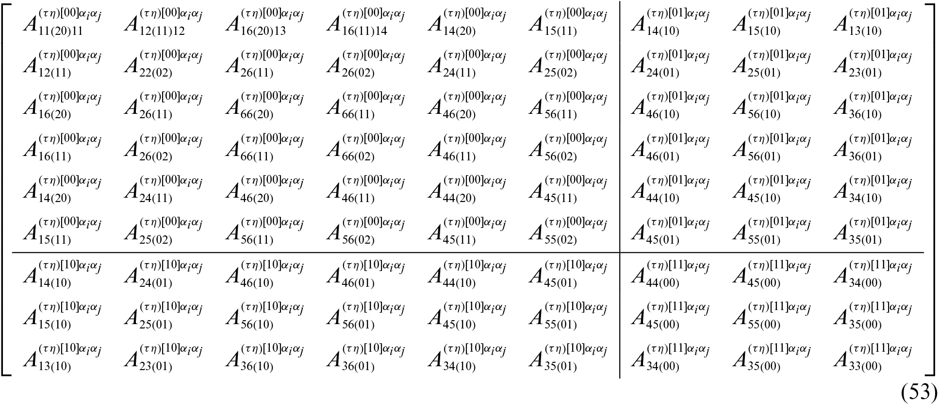
whose generic component A nm  (pq)(τη)[ fg ]α iα j is defined as:

Anm  (pq)(τη)[ fg ]α iα j=∑k=1l∫ζ kζ k+1B¯ nm(k)∂fF ηα j∂ζf∂gF τα i∂ζgH 1H 2H 1pH 2qdζ           τ,η=0,...,N+1           n,m=1,...,6for     p,q=0,1,2           α i,α j=α 1,α 2,α 3           f,g=0,1(54)

being Fηαj=∂0Fηαj/∂0Fηαj∂ζ0∂ζ0 and Fταi=∂0Fταi/∂0Fταi∂ζ0∂ζ0. As can be seen, four blocks can be traced in Eq. (53) accounting for the presence of the derivatives of the f,g-th order within the expression reported in Eq. (54). Furthermore, in Eq. (54) the term B¯nm(k) refers to the 3D rotated stiffness coefficient E¯ij(k) introduced in Eq. (51), possibly adjusted by the shear correction factor κ(ζ) [16] in the case of displacement thickness functions employed in Eq. (26) neglecting the out-of-plane stretching effects:

B¯nm(k)={E¯nm(k)forn,m=1,2,3,6κ(ζ)E¯nm(k)forn,m=4,5(55)

Employing the kinematic relations performed in Eq. (46) utilizing the generalized interpolation, Eq. (52) gets into:

S(τ)αi=∑η=0N+1∑j=13A(τη)αiαjBαju¯(η)    for    τ=0,...,N+1,   α i=α 1,α 2,α 3 (56)

Thus, the generalized ESL assessment of the constitutive relationship performed in Eq. (56) can be expressed so that each component of S(τ)αi(α1,α2) can be expressed in terms of the generalized displacement field component vector u¯(η) for η=0,…,N+1 at each point of the 2D discrete grid alongside the physical domain. Eventually, one gets:

S(τ)αi=∑η=0N+1∑j=13A(τη)αiαjDΩαjNTu¯(η)=∑η=0N+1∑j=13O(τη)αiαjNTu¯(η)for    τ=0,…,N+1,αi=α1,α2,α3(57)

In Appendix A, the interested reader can find the complete expressions for each component of matrix O(τη)αiαj.

6  Equilibrium Relations in the Variational Form

In the present section, the equilibrium equations for an arbitrary doubly-curved shell are derived by employing an energy approach. The stationary configuration is specifically enforced to the total potential energy virtual variation δΠ. The contribution of external loads should be inserted within the ESL framework, accounting for various pre-determined distributions along the top (ζ=+h/h22) and the bottom (ζ=−h/h22) surfaces of the shell. Moreover, the formulation embeds the contribution of linear elastic springs distributed along the shell edges. Suppose we denote with Les,Leb the virtual work of surface loads and boundary springs, respectively, the equilibrium configuration satisfies the following equation, accounting for the stationary assessment of the virtual variation δ of the computed quantities [16]:

δΠ=δΦ−δLes−δLeb=0(58)

being Φ the total elastic strain energy of the 3D solid, expressed via the ESL definition of the displacement field, as reported in Eq. (39).

6.1 Elastic Strain Energy

We focus on the total elastic strain energy Φ of the 3D shell described according to the ESL approach of Eq. (2). The virtual variation of Φ can be computed in terms of the 3D stress and strain vectors σ(k) and ε(k) defined in each k-th lamina of the stacking sequence concerning the geometrical principal reference system O′α1α2ζ, according to the following relation:

δΦ=∑k=1l∫α1∫α2∫ζkζk+1(δε(k))Tσ(k)A1A2H1H2dα1dα2dζ(59)

Employing the ESL assessment of the displacement field of Eq. (26), the through-the-thickness integration performed in Eq. (59) is avoided. Thus, δΦ can be computed in terms of S(τ)αi and ε(τ)αi, leading to [16]:

δΦ=∑τ=0N+1∑i=13∫α1∫α2(δε(τ)αi)TS(τ)αiA1A2dα1dα2(60)

Taking into account the weak formulation expression of generalized strain resultant vector of Eq. (46) in the previous equation, the virtual variation of the total elastic strain energy reads as:

δ Φ=∑τ=0N+1∑η=0N+1∑i=13∑j=13∫α 1∫α 2(Bα iδu¯(τ))TA(τη)α iα j(Bα ju¯(η))A 1A 2dα 1dα 2          =∑τ=0N+1∑η=0N+1(δu¯(τ))T(∑i=13∑j=13∫α 1∫α 2(Bα i)TA(τη)α iα j(Bα j)A 1A 2dα 1dα 2)u¯(η)(61)

In Eq. (61) the global stiffness matrix KΦ(τη) of the doubly-curved shell is introduced. Referring to the generic τ,η-th kinematic orders, KΦ(τη) takes the following expanded form [16]:

KΦ(τη)=∫α1∫α2[(Bα1)TA(τη)α1α1Bα1(Bα1)TA(τη)α1α2Bα2(Bα1)TA(τη)α1α3Bα3(Bα2)TA(τη)α2α1Bα1(Bα2)TA(τη)α2α2Bα2(Bα2)TA(τη)α2α3Bα3(Bα3)TA(τη)α3α1Bα1(Bα3)TA(τη)α3α2Bα2(Bα3)TA(τη)α3α3Bα3]A1A2dα1dα2=∫α1∫α2[KΦ(τη)α1α1KΦ(τη)α1α2KΦ(τη)α1α3KΦ(τη)α2α1KΦ(τη)α2α2KΦ(τη)α2α3KΦ(τη)α3α1KΦ(τη)α3α2KΦ(τη)α3α3]A1A2dα1dα2(62)

In Appendix B, an extended expression of each stiffness matrix coefficient KΦ(τη)αiαj is reported, setting τ,η=0,…,N+1 and αi,αj=α1,α2,α3.

6.2 External Loads General Distributions

Let us consider two generic vectors qa(1) and qa(2) of external loads applied to the doubly-curved shell structure at issue, whose components are referred in the above discussed geometric reference system O′α1α2ζ as shown in Fig. 2:

q a(1)=[ q 1a(1)   q 2a(1)   q 3a(1) ]T=[ q 1a(+)   q 2a(+)   q 3a(+) ]Tq a(2)=[ q 1a(2)   q 2a(2)   q 3a(2) ]T=[ q 1a(−)   q 2a(−)   q 3a(−) ]T(63)

where symbols (+) and (−) account for quantities referred to ζ=+h/h22 and ζ=−h/h22, respectively. Accordingly, a general variation q¯(α1,α2) dependent on in-plane principal coordinates can be assigned to each component qia(j) for i=1,2,3 and j=1,2 of external load vectors introduced in Eq. (63). If we denote with qi(j) a reference scaling value of loads applied along the αi principal direction, the following relation can be assessed (Fig. 2):

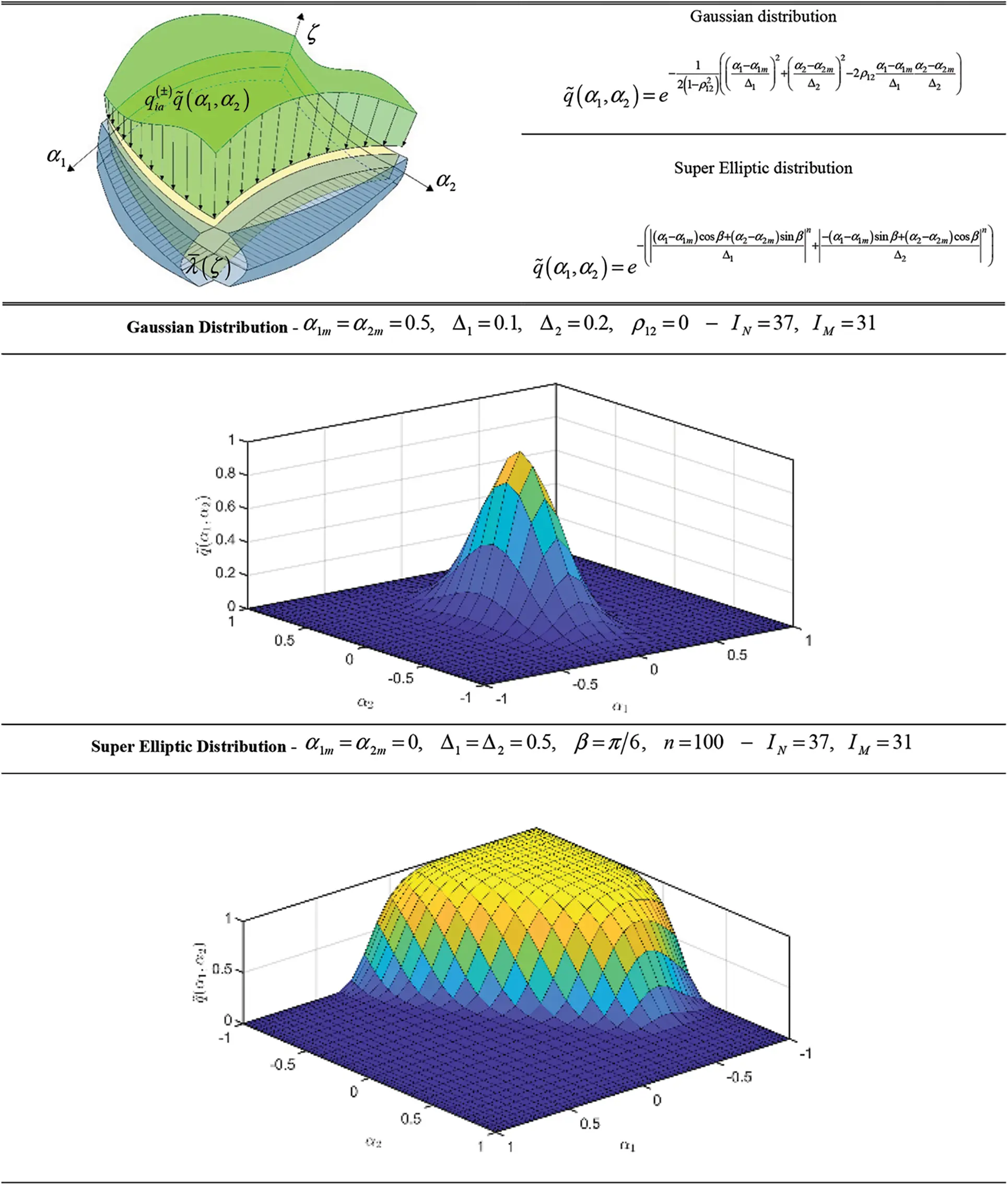
Figure 2: Generalized 2D distributions q~(α1,α2) along shell curvilinear principal coordinates α1,α2

qia(j)(α1,α2,±h2)=qi(j)|ζ=±h/2q¯(α1,α2)       for  i=1,2,3j=1,2    (64)

For a constant loading distribution, it is:

q¯(α1,α2)=1(65)

In the present manuscript, two different distributions for qa(j) components with j=1,2 are declared. A bivariate Gaussian distribution is now reported:

q¯(α1,α2)=e−12(1−ρ122)((α1−α1mΔ1)2+(α2−α2mΔ2)2−2ρ12α1−α1mΔ1α2−α2mΔ2)(66)

being αim for i=1,2 the position parameter acting on the αi in-plane principal direction with a variance scaling factor equal to Δi and a correlation factor between α1,α2 denoted with ρ12. In the same way, a Super Elliptic distribution has been employed, according to the following expression:

q¯(α1,α2)=e−(|(α1−α1m)cos⁡β+(α2−α2m)sin⁡βΔ1|n+ |−(α1−α1m)sin⁡β+(α2−α2m)cos⁡βΔ2|n)(67)

where β is the angular orientation of the bivariate dispersion principal axes of length Δi for i=1,2 with respect to α1,α2 principal shell coordinates. In addition, (α1m,α2m) is the location in the physical domain of the centre of the ellipse, whereas n is a power exponent. For n=2, Eq. (67) turns into the well-known Elliptic distribution. In Fig. 2 we plot the distributions presented in Eqs. (66) and (67), for fixed parameters configurations.

If a virtual variation δU(j) of the 3D displacement vector referred to the top (j=1) and the bottom (j=2) surface is considered, the virtual work δLes(3D) of surface loads of Eq. (63) can be computed as:

δLes(3D)=∫α1∫α2(∑j=12(∑i=13qi(j)δUi(j))H1(j)H2(j))A1A2dα1dα2(68)

being Hi(j) for j=1,2 the through-the-thickness curvature parameters calculated by means of Eq. (7) for ζ=+h/h22 and ζ=−h/h22. On the other hand, if we consider a virtual variation δu(τ) of the generalized displacement field component vector introduced in Eq. (26), a new generalized vector of external actions q(τ)(α1,α2)=[q1(τ)q2(τ)q3(τ)]T lying on the reference surface can be introduced for each τ=0,…,N+1. Thus, the virtual work δLes reads as follows:

δLes=∑τ=0N+1∫α1∫α2∑i=13qi(τ)δui(τ)A1A2dα1dα2=∑τ=0N+1∫α1∫α2(δu(τ))Tq(τ)A1A2dα1dα2(69)

The static equivalence principle employs both Eqs. (68) and (69), so that [16]:

δLes(3D)=δLes(70)

Starting from Eq. (70), the extended expressions of the q(τ) components are obtained for the τ-th kinematic expansion order, being Fταi(j) for j=1,2 the thickness function employed for the assessment of the displacement field components according to Eq. (26) calculated at ζ=+h/h22 and ζ=−h/h22, respectively:

qi(τ)=∑j=12qi(j)Fταi(j)H1(j)H2(j)fori=1,2,3(71)

Since the generalized displacement field component vectors u(τ) with τ=0,…,N+1 have been interpolated with a generalized shape functions set N in Eq. (39), the virtual work δLes of generalized external actions already computed in Eq. (69) should be expressed in terms of u¯(τ) vector taking into account Eq. (32), leading to the following expression [16]:

δLes=∑τ=0N+1∫α1∫α2(NTδu¯(τ))Tq(τ)A1A2dα1dα2=∑τ=0N+1(δu¯(τ))TQ(τ)(72)

In Eq. (72), the generalized external actions referred to each τ-th order have been collected in the 3INIM×1 column vector Q(τ), defined as:

Q(τ)=∫α1∫α2[N¯q1(τ)N¯q2(τ)N¯q3(τ)]A1A2dα1dα2(73)

6.3 Boundary Springs

The last contribution to the total potential energy occurring in Eq. (58) accounts for the influence of the elastic constraints distributed along the edges of the structure. In particular, a set of linear elastic springs of stiffness kif(k)αjm orientated along the shell side located at αj=αjm with αj=α1,α2,α3 and m=0,1 distributed along the αi=α1,α2,α3 principal direction has been considered, according to the theoretical development reported in reference [16]. The superscript k stands for the stacking sequence layer. Accordingly, they induce some boundary stresses after applying the corresponding 3D displacement component Ui=U1,U2,U3. If the physical domain consists of a rectangular 2D interval [α10,α11]×[α20,α21], different stresses are induced on each boundary. Referring to α1=α1m for m=0,1, the following definitions can be stated at the k-th lamina level, setting α2∈[α20,α21]:

σ¯1(k)(α1m,α2,ζ)=−k1f(k)α1mf(α1m,α2)U1(α1m,α2,ζ)τ¯12(k)(α1m,α2,ζ)=−k2f(k)α1mf(α1m,α2)U2(α1m,α2,ζ)for m=0,1k=1,…,lτ¯13(k)(α1m,α2,ζ)=−k3f(k)α1mf(α1m,α2)U3(α1m,α2,ζ)(74)

where f(α1m,α2) accounts for an arbitrary univariate function in the α2 coordinate located at α1=α1m. On the other hand, stresses τ¯12(k),σ¯2(k),τ¯23(k) can be found at α2=α2m according to the following definitions:

τ¯12(k)(α1,α2m,ζ)=−k1f(k)α2mf(α1,α2m)U1(α1,α2m,ζ)σ¯2(k)(α1,α2m,ζ)=−k2f(k)α2mf(α1,α2m)U2(α1,α2m,ζ)form=0,1k=1,…,lτ¯23(k)(α1,α2m,ζ)=−k3f(k)α2mf(α1,α2m)U3(α1,α2m,ζ)(75)

being α1∈[α10,α11]. In the same way, Eq. (75) contains a univariate dispersion of linear elastic springs denoted with f(α1,α2m) for α2=α2m. In order to provide an effective expression of both f(α1m,α2) and f(α1,α2m) regardless of the actual dimension of the physical domain, a new dimensionless coordinate ξ¯∈[0,1] is introduced, according to the following definition:

ξ¯=αr−αr0αr1−αr0for r=1,2(76)

As a matter of fact, the Super Elliptic distribution (S) of the p-th order has been employed, according to the following analytical expression, setting ξ¯m∈[0,1] and ξ~m∈]0,1] the position and the scaling parameter, respectively:

f(ξ)=e−(ξ¯−ξ¯mξ~m)p(77)

In the following, the expression of a Double–Weibull distribution (D) has been reported in terms of ξ¯:

f(ξ)=1−e−(ξ¯ξ¯m)p+e−(1−ξ¯ξ~m)p(78)

where ξ¯m,ξ~m∈[0,1] are two position parameters and p is the scaling value.

Starting from Eqs. (74) and (75) which have been expressed for a 3D structure, the stresses coming from the linear elastic springs distributions should be computed in terms of generalized stress resultants, accounting for the ESL assessment of the displacement field. Substituting Eq. (26) in the previously cited relations, one gets for α1=α1m with m=0,1:

[N¯1(τ)α1N¯12(τ)α2T¯1(τ)α3]=−∑η=0N+1[L1(2)α1mfb(τη)α1000L2(2)α1mfb(τη)α2000L3(2)α1mfb(τη)α3][u1(η)u2(η)u3(η)]=−∑η=0N+1L(1)α1mfb(τη)u(η)for m=0,1forα2∈[α20,α21](79)

Referring to the edges of the structure located at α2=α2m for m=0,1, Eq. (75) turns into:

[ N¯ 21(τ)α1N¯ 2(τ)α2T¯ 2(τ)α3 ]=−∑η=0N+1[ L 1(1)α 2mfb(τη)α 1000L 2(1)α 2mfb(τη)α 2000L 3(1)α 2mfb(τη)α 3 ][ u 1(η)u 2(η)u 3(η) ]=−∑η=0N+1L (1)α 2mfb(τη)u (η)       for   m=0,1               for   α 1∈[ α 20,α 21 ](80)

Fundamental coefficients Li(p)αnmfb(τη)αi occurring in Eqs. (79) and (80) can be computed for each τ,η=0,…,N+1 according to the following relation, setting n,p=1,2, i=1,2,3 and n,p=1,2:

Li(p)αnmfb(τη)αi=∑k=1l∫ζkζk+1kif(k)αnmFηαiFταiHpdζ(81)

Having in mind the ESL assessment of general distributions of boundary springs, the virtual work contribution δLeb to Eq. (58) can be computed as the sum of δLeb1 and δLeb2, referred to the edges of the physical domain characterized by α1=α1m and α2=α2m, respectively, for m=0,1 [16]:

δLeb=δLeb1+δLeb2=∑τ=0N+1(∮α2(δu(τ))TS¯α1(τ)A2α2+∮α1(δu(τ))TS¯α2(τ)A1α1)(82)

where S¯α1(τ) components are defined according to what exerted in Eq. (80). S¯α2(τ) accounts for the generalized boundary stressed reported in Eq. (80). Introducing in Eq. (82) the weak form assessment of the displacement field of Eq. (32), the final form of δLeb comes out:

δLeb=δLeb1+δLeb2=∑τ=0N+1((δu¯(τ))T(Q¯α1(τ)+Q¯α2(τ)))(83)

being Q¯α1(τ),Q¯α2(τ) the ESL boundary load vectors of Eqs. (79) and (80) expressed in terms of the generalized interpolation of the displacement field, as follows [16]:

Q¯α1(τ)=∮α2[N¯N¯1(τ)α1N¯N¯12(τ)α2N¯T¯1(τ)α3]A2α2,Q¯α2(τ)=∮α1[N¯N¯21(τ)α1N¯N¯2(τ)α2N¯T¯2(τ)α3]A1α1(84)

Thus, the generalized displacement vector u¯(τ) of Eq. (32) can be outlined in Eq. (83), accounting for the definitions of Eq. (84), together with what has been exerted in Eqs. (79) and (80). The final form of the virtual work associated with boundary springs reads as:

δLeb=∑τ=0N+1(δu¯(τ))T∑η=0N+1(∑m=01(∮α2NL(1)α2mfb(τη)NTA2α2+∮α1NL(1)α1mfb(τη)NTA1α1))u¯(η)=∑τ=0N+1(δu¯(τ))T∑η=0N+1K¯b(τη)u¯(η)(85)

Note that the fundamental stiffness matrix K¯b(τη) has been introduced, accounting for the ESL generalized stresses induced by the springs distributed along the edges of the physical domain, at each τ,η=0,…,N+1 kinematic expansion order, as well as the generalized shape functions arranged in N, based on the Lagrange interpolation procedure of Eq. (32).

6.4 Fundamental Governing Equations

The final form of the fundamental governing equations of the static problem can be outlined from Eq. (58), taking into account the contributions of the elastic strain energy of Eq. (61), the virtual work of surface loads of Eq. (72) and that of external boundary springs of Eq. (85). Referring to the τ-th order of the kinematic expansion, one gets [16]:

∑η=0N+1(K¯Φ(τη)−K¯b(τη))u¯(η)=Q(τ)⇔∑η=0N+1K¯(τη)u¯(η)=Q(τ)forτ=0,…,N+1(86)

In extended form, Eq. (86) can be assembled with respect to the displacement field ESL higher order model of Eq. (26), leading to the following expression:

[K¯(00)K¯(01)⋯K¯(0(N))K¯(0(N+1))K¯(10)K¯(11)⋯K¯(1(N))K¯(1(N+1))⋮⋮⋱⋮⋮K¯((N)0)K¯((N)1)⋯K¯((N)(N))K¯((N)(N+1))K¯((N+1)0)K¯((N+1)1)⋯K¯((N+1)(N))K¯((N+1)(N+1))][U¯(0)U¯(1)⋮U¯(N)U¯(N+1)]=[Q(0)Q(1)⋮Q(N)Q(N+1)]⇔K¯u¯=Q(87)

For shells of arbitrary shapes, the employment of the generalized blending functions assessed in Eq. (13) with the Jacobian matrix J of the transformation defined in Eq. (17) should be taken into account in the computation of all the contributions of Π occurring in Eq. (58). Accordingly, the generalized stiffness matrix K¯(τη) and the external surface loads Q(τ) should be adjusted appropriately for each τ=0,…,N+1 since integrals with respect to principal directions α1,α2 should be assessed in terms of natural coordinates ξ1,ξ2∈[−1,1]. Referring to a specific τ th kinematic expansion order, stiffness matrix defined in Eq. (62) turns into the following relation:

KΦ(τη)=∫−11∫−11[KΦ(τη)α1α1KΦ(τη)α1α2KΦ(τη)α1α3KΦ(τη)α2α1KΦ(τη)α2α2KΦ(τη)α2α3KΦ(τη)α3α1KΦ(τη)α3α2KΦ(τη)α3α3]A1A2det(J)dξ1dξ2(88)

The ESL assessment of external surface load vector Q(τ) reported in Eq. (73) reads as follows [16]:

Q(τ)=∫−11∫−11[N¯q1(τ)N¯q2(τ)N¯q3(τ)]A1A2det(J)dξ1dξ2(89)

As far as the definition of generalized boundary springs for arbitrarily-shaped structures is concerned, it is useful to refer to the local coordinate system introduced in Eq. (11) along each edge of the shell. As a consequence, boundary stresses can be expressed with respect to nn,ns,nζ directions employing the symbols N¯n(τ)α1,N¯ns(τ)α2,T¯ζ(τ)α3. The generalized boundary springs along the i-th edge of the structure with i=1,…,4 accounts as:

Q¯ n(i)(τ)=∫0L(i)[ N¯N¯ n(τ)α 1N¯N¯ ns(τ)α 2N¯T¯ ζ(τ)α 3 ] dsn(i)      for    i=1,...,4          τ=0,...,N+1(90)

Starting from the blending coordinates transformation of Eq. (13), the length L(i) of the shell side can be computed according to the following relation [16], setting j=1,2:

L(i)=∫−11A12(dα1dξj)2+A22(dα2dξj)2dξjfori=1,…,4(91)

Since the natural coordinate set ξ1,ξ2 has been defined in the dimensionless rectangular interval [−1,1]×[−1,1], Eq. (90) can be written as:

Q¯n(i)(τ)=∫−11[N¯N¯n(τ)α1N¯N¯ns(τ)α2N¯T¯ζ(τ)α3]L(i)2dη(i)fori=1,..,4(92)

Once the quantity Q¯n(i)(τ) has been successfully computed in the previous equation for each τ-th order, a kinematic expansion is performed such that Eq. (92) is embedded in the global variational matrices of Eq. (87). In this way, the global stiffness matrix K¯ accounts for the 3D assessment of the boundary linear elastic springs introduced for the definition of natural and non-conventional boundary conditions, whereas the term Q is employed for the external surface loads.

In order to compute the generalized stress resultants N¯n(τ)α1,N¯ns(τ)α2,T¯ζ(τ)α3 induced by linear elastic springs for a mapped geometry employing the approach of Eqs. (74) and (75), it is useful to express the generalized displacement field un(τ),us(τ),uζ(τ) referred to nn,ns,nζ local reference system in terms of u1(τ),u2(τ),u3(τ) for each τ-th order of the kinematic expansion [16]:

[un(τ)us(τ)uζ(τ)]=[nn1nn20ns1ns20001][u1(τ)u2(τ)u3(τ)](93)

In the same way, the generalized stress resultants N¯n(τ)α1,N¯ns(τ)α2,T¯ζ(τ)α3 should be expressed in terms of the S(τ)αi vector for αi=α1,α2,α3 according to the following relations [16]:

[Nn(τ)α1Nns(τ)α2Tζ(τ)α3]=[nn12nn22nn1nn2nn1nn200nn1ns1nn2ns2nn1ns2nn2ns1000000nn1nn2][N1(τ)α1N2(τ)α1N12(τ)α1N21(τ)α1T1(τ)α3T2(τ)α3](94)

7  Numerical Implementation with the GDQ Method

In the present section we deal with the numerical assessment of the fundamental governing equations for the static problem derived in Eq. (87) in their assembled form. The employed numerical technique that has been adopted is the well-known GDQ method. According to this methodology, the discrete form of the derivatives is directly provided. Referring to a generic point (ξ1,ξ2)∈[−1,1]×[−1,1] belonging to the dimensionless squared computational domain, the (n+m)-th order derivative of a bivariate function f(ξ1,ξ2) concerning natural coordinates ξ1,ξ2 can be expressed as [16]:

∂n+mf(ξ 1,ξ 2)∂ξ 1n∂ξ 2m|ξ 1=ξ1i, ξ 2=ξ2j≅∑k=1I Nςikξ 1(n)(∑l=1IMςjlξ 2(m)f(ξ 1k,ξ 2l))   i = 1, 2,..., INj = 1, 2,..., IM(95)

where IN,IM denote the number of the selected discrete points along ξ1,ξ2 directions, respectively. As can be seen, Eq. (95) accounts for a quadrature rule for derivative purposes. The weighting coefficients ςpvξr(q) for r=1,2, p=i,j, q=n,m and v=k,l are computed utilizing the recursive expression valid for each q≥1 [16]:

ςpvξ r(1)=L(1)(ξ rp)(ξ rp−ξ rv)L(1)(ξ rv),          ςpvξ r(q)=q(ςpvξ r(1)ςppξ r(q−1)−ςpvξ r(q−1)ξ rp−ξ rv)p≠vςppξ r(q)=−∑v=1 v≠pNςpvξ r(q)p=v(96)

Eq. (96) is based on the interpolation of the unknown function employing the Lagrange interpolating polynomials L. In the case of pure derivatives with respect to ξ1,ξ2, it gives m=0 and n=0, respectively, and GDQ coefficients come into the following relation:

ςpvξr(0)=δpvforr=1,2(97)

being δpv the Kronecker delta operator. For a generic non-uniform grid of IN×IM points, the GDQ weighting coefficients for the derivative of the (n+m)-th order are calculated by means of Eqs. (96) and (97) are collected in a INIM×INIM squared matrix denoted with ςξ1(n)ξ2(m). Starting from Eq. (96), the matrix at issue can be obtained from a proper expansion of matrix ςξr(q) for q=n,m and r=1,2 of dimensions IQ×IQ with IQ=IN,IM, respectively, accounting for the derivatives of n-th and m-th order along ξ1,ξ2:

ςξ1(n)ξ2(m)=ςξ2(m)⊗ςξ1(n)(98)

Based on Eq. (97), it is ςξr(0)=I. In this way, the numerical derivation employing the GDQ method with respect to ξ1,ξ2 can be performed as:

f→(n+m)=ςξ1(n)ξ2(m)f→(99)

where f is a IN×IM matrix whose general component is f(ξ1i,ξ1j) for i=1,…,IN and j=1,…,IM. In the same way, the generic element of f(n+m) is ∂n+mf(ξ1i,ξ2j)/∂n+mf(ξ1i,ξ2j)∂ξ1n∂ξ2m∂ξ1n∂ξ2m.

A 2D Legendre-Gauss-Lobatto (LGL) grid of dimensions IN×IM referred to the domain [−1,1]×[−1,1] has been here adopted, such that:

(1−ξ r2)A I​P−1(ξ r)=0      for    I P=I N,I Mr=1,2           (100)

In Eq. (100), AIP−1(ξr) with r=1,2 denotes the Lobatto polynomials of the IP-th order, which can be calculated from the IP-th derivation of the Legendre polynomials LIP−1(ξr) with respect to ξr [16]:

A I​P−1(ξ r)=ddξ r(L I​P(ξ r))      for    I P=I N,I M        r=1,2                    ξ r∈[ −1,1 ]             (101)

Since the fundamental governing relations (86) account for derivations along α1,α2 principal directions, we consider the GDQ rule of Eq. (95) referred to natural coordinates ξ1,ξ2. The matrix approach is then followed, starting from Eq. (98). Employing the generalized blending functions reported in Eq. (13), the matrices ςα1(1)α2(0) and ςα1(0)α2(1) for the first order derivatives along α1,α2 of a generic bivariate function f(α1,α2) can be computed as:

ςα 1(1)α 2(0)=P→ 11∘ςξ 1(1)ξ 2(0)+P→ 21∘ςξ 1(0)ξ 2(1)ςα 1(0)α 2(1)=P→ 12∘ςξ 1(1)ξ 2(0)+P→ 22∘ςξ 1(0)ξ 2(1)(102)

being P→ij with i,j=1,2 the vectorized form by means of Eq. (29) of the coordinate transformation computed by Eq. (19). In the same way, starting from Eq. (22) and Eq. (24) the discrete form of second order derivatives can be assessed introducing the quantities Prij with r,i,j=1,2:

ςα1(2)α2(0)=P→11o2∘ςξ1(2)ξ2(0)+P→21o2∘ςξ1(0)ξ2(2)+2P→11∘P→21∘ςξ1(1)ξ2(1)+P→111∘ςξ1(1)ξ2(0)+P→211∘ςξ1(0)ξ2(1)ςα1(0)α2(2)=P→12o2∘ςξ1(2)ξ2(0)+P→22o2∘ςξ1(0)ξ2(2)+2P→12∘P→22∘ςξ1(1)ξ2(1)+P→122∘ςξ1(1)ξ2(0)+P→222∘ςξ1(0)ξ2(1)ςα1(1)α2(1)=P→11∘P→12∘ςξ1(2)ξ2(0)+P→21∘P→22∘ςξ1(0)ξ2(2)+(P→11∘P→22+P→12∘P→21)∘ςξ1(1)ξ2(1)+P→112∘ςξ1(1)ξ2(0)+P→212∘ςξ1(0)ξ2(1)(103)

The employment of the GDQ method allows to obtain the discrete form of the governing equations. When the assembly of the fundamental relations is performed alongside the entire IN×IM computational domain, it is useful to distinguish the inner domain nodes “d” from those located along the boundaries (“b” nodes). As a matter of fact, the DOFs associated with the latter are collected in a column vector denoted with δb, whereas those referring to the former are arranged within the vector δd. Thus, the fundamental system accounts as follows [16]:

[K¯bbK¯bdK¯dbK¯dd][δbδd]=[Q¯bQ¯d](104)

Performing a static condensation of Eq. (104) with respect to δd according to the procedure reported in Eq. (16), the final form of the discrete system of dimensions 3(N+2)INIM×3(N+2)INIM comes out, being I the identity matrix:

(K¯dd−K¯db(K¯bb)−1K¯bd)δd=Q¯d−K¯db(K¯bb)−1Q¯b(105)

The numerical integrations that are involved in the formulation of the present manuscript are performed by means of the GIQ procedure [16]. Referring to a generic univariate function f=f(x) defined in the closed interval [a,b] with a<b∈R, a discrete grid is selected from the 1D domain, namely xk∈[a,b] with k=1,2,…,IN. Accordingly, the integral of f restricted to the sub-interval [xi,xj]⊆[a,b] with xi,xj belonging to the grid at issue can be computed as a weighted sum of the values f(xk) for k=1,2,…,IN assumed by the function at each point of the computational grid of [a,b]:

∫xixjf(x)dx=∑k=1INwkijf(xk)(106)

where wkij=wjk−wik are referred to the interval [xi,xj]. The coefficients wjk,wik are computed following the extensive procedure of reference [16], starting from the shifted GDQ weighting coefficients reported hereafter, setting ε=1×10−10:

ς¯ ijζ(1)=ζ i−εζ j−ες ijζ(1)            for   i≠jς¯ ijζ(1)=ς iiζ(1)+1ζ i−ε       for   i=j(107)

Then, they are collected in the matrix ς¯ζ(1) of dimensions IN×IN. Thus, the coefficients wik,wjk referred to the integral of f restricted to the interval [ε,xr]⊆[a,b] are the elements of the GIQ matrix, reading as:

W=(ς¯ζ(1))−1(108)

All the terms wkij introduced in Eq. (106) can be collected in a vector of dimensions 1×IN denoted with w(x), setting x the integration variable. In the same way, the 1×IM vector w(y) can be introduced when the integration of the univariate function f=f(y) is required. For a bivariate function f=f(x,y), Eq. (106) turns into the following expression, setting a generic 2D IN×IM grid from a rectangular domain [a,b]×[c,d] of extremes a<b∈R and c<d∈R [16]:

∫cd∫abf(x,y)dxdy=∑i=1IN∑j=1IMwi1INwj1IMf(xi,yj)=∑k=1INMwk1INMfk(109)

where fk values for k=1,…,INM=INIM are arranged employing the above introduced by-column vectorization operation of Eq. (29). On the other hand, wk1INIM GIQ coefficients are computed using the previously introduced vectors w(x),w(y), as reported:

w(xy)=w(y)⊗w(x)=[w11IM⋯wIM1IM]⊗[w11IN⋯wIN1IN](110)

Referring to the bivariate function f=f(x,y), it is also possible performing a univariate integration along a parametric line of the rectangular computational domain parallel to x and y, respectively, employing the GIQ rule. For this purpose, w(x0) and w(0y) are defined starting from Eq. (110):

w(0y)=w(y)⊗o(x)w(x0)=o(y)⊗w(x)(111)

For the sake of completeness, symbol o(x),o(y) are row vectors of ones of dimensions 1×IN and 1×IM, respectively. Thus, the following relations can be derived:

∫abf(x,y)dx=∑i=1IN∑j=1IMwi1INwj(0)f(xi,yj)∫cdf(x,y)dy=∑i=1IN∑j=1IMwi(0)wj1IMf(xi,yj)(112)

We recall that in Eq. (87) the global stiffness matrix of the shell has been provided, starting from a parametrization of the reference surface r(α1,α2) employing principal coordinates. As it has been shown, for arbitrarily-shaped structures KΦ(τη) for τ,η=0,…,N+1 is described by means of natural coordinates ξ1,ξ2 in Eq. (88). For this purpose, it is useful to define a matrix of dimensions 3INIM×3IN2IM2 for the transformation at issue:

P=(w(ξ1ξ2)∘(A→1∘A→2∘D→J)T)⊗O(113)

being O a ones squared matrix of dimensions 3INIM. Accordingly, w(ξ1ξ2)=w(ξ2)⊗w(ξ1) following Eq. (110), whereas DJ, A1, and A2 accounts for the determinant of the Jacobian matrix J, as well as the Lamè parameters A1,A2 of the shell. If the index k=n+(m−1)IN with n=1,…,IN and m=1,…,IM is assessed, we obtain the vectorized form of KΦ(τη), accounting for the IN×IM grid of the computational domain:

K~Φ(τη)=[KΦ(1)(τη)αiαjKΦ(2)(τη)αiαj⋯KΦ(k)(τη)αiαj⋯KΦ(INIM)(τη)αiαj]T(114)

Employing Eqs. (113) and (114), the stiffness matrix K^Φ(nm)(τη) for an arbitrarily-shaped shell structure can be computed:

K^Φ(nm)(τη)=PK~Φ(τη)(115)

In the following, the discrete form of the generalized external loads of Eq. (84) is provided by means of the GIQ method presented in Eq. (106):

N~1(τ)α1=w(0α2)T∘A→2∘N¯1(τ)α1N~12(τ)α2=w(0α2)T∘A→2∘N¯12(τ)α2T~1(τ)α3=w(0α2)T∘A→2∘T¯1(τ)α3N~21(τ)α1=w(α10)T∘A→1∘N¯21(τ)α1N~2(τ)α2=w(α10)T∘A→1∘N¯2(τ)α2T~2(τ)α3=w(α10)T∘A→1∘T¯2(τ)α3(116)

In the same way, Eq. (116) becomes suitable for an arbitrary mapped domain. According to the nomenclature introduced in Eq. (12), it gives for ξ2=−1:

N˜n(τ)α1=L(1)2w˜(α10)T∘N¯n(τ)α1N˜ns(τ)α2=L(1)2w˜(α10)T∘N¯ns(τ)α2T˜ζ(τ)α3=L(1)2w˜(α10)T∘T¯ζ(τ)α3(117)

The edge characterized by ξ1=1 behaves as:

N˜n(τ)α1=L(2)2w˜(0α2)T∘N¯n(τ)α1N˜ns(τ)α2=L(2)2w˜(0α2)T∘N¯ns(τ)α2T˜ζ(τ)α3=L(2)2w˜(0α2)T∘T¯ζ(τ)α3(118)

On the other hand, for ξ2=1 it is:

N˜n(τ)α1=L(3)2w˜(α10)T∘N¯n(τ)α1N˜ns(τ)α2=L(3)2w˜(α10)T∘N¯ns(τ)α2T˜ζ(τ)α3=L(3)2w˜(α10)T∘T¯ζ(τ)α3(119)

Finally, the edge identified with ξ1=−1 reads as:

N˜n(τ)α1=L(4)2w˜(0α2)T∘N¯n(τ)α1N˜ns(τ)α2=L(4)2w˜(0α2)T∘N¯ns(τ)α2T˜ζ(τ)α3=L(4)2w˜(0α2)T∘T¯ζ(τ)α3(120)

8  Post-Processing Analysis

Once the fundamental governing relations reported in Eq. (87) have been solved by means of the GDQ method, the solution in terms of the generalized displacement field component vector u(τ) is obtained. Actually, the 3D distributions of both kinematic and mechanical quantities along the shell thickness should be recovered starting from the outcomes of the 2D model. To this purpose, the Chebyshev-Gauss-Lobatto (CGL) non-uniform grid is introduced. The location ξg of the computational points is provided for the [−1,1] dimensionless interval [16]:

ξ g=−cos (g−1I T−1π)      for   ξ g∈[ −1,1 ]g=1,...,I T(121)

being IT the number of the selected discrete points. Referring to the interval [ζk,ζk+1] for k=1,…,l representing the k-th layer of the staking sequence within the 3D physical domain, Eq. (121) should be transformed according to the following relation:

ζg=ζ k+1−ζ k2(ξg+1)+ζ k      for   ξ g∈[ −1,1 ]g=1,...,I Tk=1,...,l(122)

Employing the unified ESL assessment of the displacement field introduced in Eq. (26) it is possible to derive the through-the-thickness distribution of the displacement field component vector U(ijg)(k) with i=1,…,IN, j=1,…,IM and g=1,…,IT for each k-th layer of the stacking sequence [16]:

U(ijg)(k)=∑τ=0N+1Fτ(g)(k)u(ij)(τ)(α1i,α2j)⇔[U1(ijg)(k)(α1i,α2j,ζg(k))U2(ijg)(k)(α1i,α2j,ζg(k))U3(ijg)(k)(α1i,α2j,ζg(k))]=∑τ=0N+1[Fτ(g)α1(k)(ζg(k))000Fτ(g)α2(k)(ζg(k))000Fτ(g)α3(k)(ζg(k))][u1(ij)(τ)(α1i,α2j)u2(ij)(τ)(α1i,α2j)u3(ij)(τ)(α1i,α2j)](123)

being Fτ(g)α1(k)(ζg(k)),Fτ(g)α2(k)(ζg(k)),Fτ(g)α3(k)(ζg(k)) the generalized thickness functions set calculated at the (α1i,α2j,ζg(k)) point of the 3D solid, whereas u1(ij)(τ),u2(ij)(τ),u3(ij)(τ) are the generalized displacement field components for the τ-th kinematic expansion order referred to the point (α1i,α2j) of the physical domain, for i=1,…,IN, j=1,…,IM. In the same way, the generalized strain component vector ε(ij)(τ)αq for q=1,2,3 and τ=0,…,N+1 are computed in terms of the discrete 3D strain component vector ε(ijg)(k)=[ε1(ijg)(k)ε2(ijg)(k)γ12(ijg)(k)γ13(ijg)(k)γ23(ijg)(k)ε3(ijg)(k)]T within each k-th lamina, leading to the following expression:

ε(ijg)(k)=∑τ=0N+1∑q=13Z(ijg)(kτ)αiε(ij)(τ)αq(124)

Referring to the generic (α1i,α2j,ζg(k)) point of the shell structure, membrane stresses can be calculated according to the generally anisotropic law of Eq. (51), leading to the following relation, setting E¯ij(kg) for i,j=1,…,6 the elastic stiffness coefficients of the k-th layer referred to the geometric reference system employed for the computation of σ1(k),σ2(k),τ12(k) stresses:

[σ1(ijg)(k)σ2(ijg)(k)τ12(ijg)(k)]=[E¯11(ijg)(k)E¯12(ijg)(k)E¯16(ijg)(k)E¯14(ijg)(k)E¯15(ijg)(k)E¯13(ijg)(k)E¯12(ijg)(k)E¯22(ijg)(k)E¯26(ijg)(k)E¯24(ijg)(k)E¯25(ijg)(k)E¯23(ijg)(k)E¯16(ijg)(k)E¯26(ijg)(k)E¯66(ijg)(k)E¯46(ijg)(k)E¯56(ijg)(k)E¯36(ijg)(k)][ε1(ijg)(k)ε2(ijg)(k)γ12(ijg)(k)γ13(ijg)(k)γ23(ijg)(k)ε3(ijg)(k)](125)

Nevertheless, the remaining stress components τ13(k),τ23(k),σ3(k) are not calculated starting from the constitutive relation (51). The 3D equilibrium equations [16] expressed in curvilinear principal coordinates are employed, instead, as:

[∂∂ζ+1R1+ζ+1R2+ζ000∂∂ζ+1R1+ζ+1R2+ζ000∂∂ζ+1R1+ζ+1R2+ζ][τ13(k)τ23(k)σ3(k)]=[a(k)b(k)c(k)](126)

where R1,R2 are the principal curvature radii of the reference surface r(α1,α2), whereas the terms a(k),b(k),c(k) depend on the quantities calculated in Eq. (125), reading as:

a(k)=−1A 1(1+ζ/R 1)∂σ 1(k) ∂α 1+σ 2(k)−σ 1(k) A 1A 2(1+ζ/R 2)∂A 2∂α 1−1A 2(1+ζ/R 2)∂τ 12(k) ∂α 2−2τ 12(k)A 1A 2(1+ζ/R 1)∂A 1∂α 2b(k)=−1A 2(1+ζ/R 2)∂σ 2(k)∂α 2+σ 1(k)−σ 2(k)A 1A 2(1+ζ/R 1)∂A 1∂α 2−1A 1(1+ζ/R 1)∂τ 12(k) ∂α 1−2τ 12(k)A 1A 2(1+ζ/R 2)∂A 2∂α 1c(k)=−1A 1(1+ζ/R 1)∂τ 13(k)∂α 1−τ 13(k)A 1A 2(1+ζ/R 2)∂A 2∂α 1−1A 2(1+ζ/R 2)∂τ 23(k) ∂α 2−τ 23(k)A 1A 2(1+ζ/R 1)∂A 1∂α 2+σ 1(k)R 1+ζ+σ 2(k)R 2+ζ(127)

It should be noted that the expression of c(k) contains the terms τ13(k),τ23(k). For this reason, the first two relations of Eq. (126) should be solved independently in the first step. Then, the solution of the third equation can be easily found. To this end, the discrete form of the derivatives of in-plane stresses σ1(k),σ2(k),τ12(k) with respect to α1,α2 occurring in the first two expressions of Eq. (127) should be performed employing the GDQ method for each k-th layer of the lamination scheme, setting k=1,…,l:

 σ1,1(ijg)(k)=∂σ 1(k)∂α 1|(ijg)≅∑q=1I Nς iqα 1(1)σ 1(qjg)(k),        σ2,2(ijg)(k)=∂σ 2(k)∂α 2|(ijg)≅∑q=1I Mς jqα 2(1)σ 2(qjg)(k)τ12,1(ijg)(k)=∂τ 12(k)∂α 1|(ijg)≅∑q=1I Nς iqα 1(1)τ 12(qjg)(k),        τ12,2(ijg)(k)=∂τ 12(k)∂α 2|(ijg)≅∑q=1I Mς jqα 2(1)τ 12(qjg)(k)(128)

The first order differential relations (126) should fulfill a single boundary condition. Referring to the first lamina of the stacking sequence (k=1), the external loads applied at the bottom side of the structure (ζ=−h/h22) satisfy the following boundary conditions:

τ~13(ij1)(1)=q1a(ij)(−)τ~23(ij1)(1)=q2a(ij)(−)(129)

being q1a(ij)(−),q2a(ij)(−) the in-plane static loads referred to the (α1i,α2j) point of the bottom skin of the structure following the convention in Eq. (63). On the other hand, for an arbitrary k-th layer, the first two relations of Eq. (126) can be solved at each discrete grid point (α1i,α2j,ζg(k)) by means of the GDQ computations of Eq. (128) enforcing the unknown stress compatibility conditions between the k-th and the (k+1)-th laminae as follows:

τ˜ 13(ijI T)(k)=τ˜ 13(ij1)(k+1)τ˜ 23(ijI T)(k)=τ˜ 23(ij1)(k+1)     for    i=1,...,I N  j=1,...,I M  k=1,...,l−1(130)

For the surface loads q1a(ij)(+) and q2a(ij)(+) at the top side, an adjustment algorithm is provided starting from the solution of Eq. (126) by means of the boundary conditions (129) and (130). Accordingly, the exact fulfilment of the compatibility conditions between stresses and in-plane external loads is ensured at the external shell skins [16]:

τ13(ijs)=τ˜13(ijs)+(ζ s+h(ij)2)q 1a(ij)(+)−τ˜13(ijIL)h(ij)τ23(ijs)=τ˜23(ijs)+(ζ s+h(ij)2)q 2a(ij)(+)−τ˜23(ijIL)h(ij)     for    i=1,...,I Nj=1,...,I Ms=1,...,I L=l⋅I T(131)

In the previous equation an index s=kg has been introduced, accounting for g=1,…,IT points defined according to Eq. (122) for the k-th lamina alongside the entire shell thickness h(ij)=h(αi,αj) for i=1,…,IN and j=1,…,IM. As a matter of fact, stresses τ~13(ijIL),τ~23(ijIL) come from the direct solution of the balance Eq. (126). The introduction of the index s leads to vectors τ~13,τ~23 employed for the numerical implementation of Eq. (131), accounting for an assembly of out-of-plane shear stresses alongside the entire lamination scheme:

τ~13=[τ~13(ij1)(1)⋯τ~13(ijIT)(1)τ~13(ij1)(2)⋯τ~13(ijIT)(2)⋯τ~13(ij1)(k)⋯τ~13(ijIT)(k)⋯τ~13(ij1)(l)⋯τ~13(ijIT)(l)]Tτ~23=[τ~23(ij1)(1)⋯τ~23(ijIT)(1)τ~23(ij1)(2)⋯τ~23(ijIT)(2)⋯τ~23(ij1)(k)⋯τ~23(ijIT)(k)⋯τ~23(ij1)(l)⋯τ~23(ijIT)(l)]T(132)

Once the corrected values τ13(ijs),τ23(ijs) of stresses are found employing Eq. (131), the index association τ13(ijm)(k)=τ13(ijs) and τ23(ijm)(k)=τ23(ijs) is performed. In this way, the first order derivatives of τ13(k),τ23(k) with respect to α1,α2 can be performed within each k-th lamina based on the GDQ algorithm:

∂τ13(k)∂α1|(ijm)≅∑q=1INςiqα1(1)τ13(qjm)(k),∂τ23(k)∂α2|(ijm)≅∑q=1IMςjqα2(1)τ23(qjm)(k)(133)

Now, it is possible to solve the third differential relation in (126), while enforcing the stress compatibility condition for the surface external loads q3a(−) at the boundary of the shell. Referring to the discrete point located at (α1i,α2j), one gets:

σ~3(ij1)(1)=q3a(ij)(−)(134)

In the same way, the following relation should be fulfilled at the interface level between the k-th and (k+1)-th lamina, being k=1,…,l−1:

σ~3(ijIT)(k)=σ~3(ij1)(k+1)(135)

Following a similar procedure to Eq. (132) for τ13(k),τ23(k) shear stresses, the association σ~3(ijm)(k)=σ~3(ijs) is performed, thus leading to the definition of the following vector:

σ~3=[σ~3(ij1)(1)⋯σ~3(ijIT)(1)σ~3(ij1)(2)⋯σ~3(ijIT)(2)⋯σ~3(ij1)(k)⋯σ~3(ijIT)(k)⋯σ~3(ij1)(l)⋯σ~3(ijIT)(l)]T(136)

Therefore, the load boundary conditions at the top surface of the shell read as [16]:

σ3(ijs)=σ~3(ijm)+(ζs+h(ij)2)q3a(ij)(+)−σ~3(ijIL)h(ij)(137)

being q3a(ij)(+) the component of external loads applied at ζ=+h/h22 at each (α1i,α2j) point.

Starting from the main outcomes of Eqs. (131) and (137), the corrected values of the out-of-plane 3D deformations collected γ13(k),γ23(k),ε13(k) of the k-th layer can be calculated as well, according to what has been stated in reference [16]. To this end, the constitutive law for generally anisotropic materials introduced in Eq. (51) is employed. Performing a computation in each discrete point (α1i,α2j,ζg(k)) with i=1,…,IN, j=1,…,IM and g=1,…,IT, it gives the discrete vector x(ijg)(k)=[γ13(ijg)(k)γ23(ijg)(k)ε3(ijg)(k)]T:

A(ijg)(k)x(ijg)(k)=b(ijg)(k)(138)

where

A(ijg)(k)=[E¯44(ijg)(k)E¯45(ijg)(k)E¯34(ijg)(k)E¯45(ijg)(k)E¯55(ijg)(k)E¯35(ijg)(k)E¯34(ijg)(k)E¯35(ijg)(k)E¯33(ijg)(k)]b(ijg)(k)=[τ13(ijg)(k)τ23(ijg)(k)σ3(ijg)(k)]−[E¯14(ijg)(k)E¯24(ijg)(k)E¯46(ijg)(k)E¯15(ijg)(k)E¯25(ijg)(k)E¯56(ijg)(k)E¯13(ijg)(k)E¯23(ijg)(k)E¯36(ijg)(k)][ε1(ijg)(k)ε2(ijg)(k)γ12(ijg)(k)](139)

From the inversion of the fundamental linear system of Eq. (138), the corrected values of γ13(ijg)(k),γ23(ijg)(k),ε3(ijg)(k) 3D strains are provided at each discrete point of the shell (α1i,α2j,ζg(k)) with i=1,…,IN, j=1,…,IM and g=1,…,IT:

γ 13(ijg)(k)=1detA(ijg)(k)(E¯ 33(ijg)(k)E¯ 55(ijg)(k)−(E¯ 35(ijg)(k))2)(τ 13(ijg)(k)−E¯ 14(ijg)(k)ε 1(ijg)(k)−E¯ 24(ijg)(k)ε 2(ijg)(k)−E¯ 46(ijg)(k)γ 12(ijg)(k))              +1detA(ijg)(k)(E¯ 34(ijg)(k)E¯ 35(ijg)(k)−E¯ 33(ijg)(k)E¯ 45(ijg)(k))(τ 23(ijg)(k)−E¯ 15(ijg)(k)ε 1(ijg)(k)−E¯ 25(ijg)(k)ε 2(ijg)(k)−E¯ 56(ijg)(k)γ 12(ijg)(k))              +1detA(ijg)(k)(E¯ 35(ijg)(k)E¯ 45(ijg)(k)−E¯ 34(ijg)(k)E¯ 55(ijg)(k))(σ 3(ijg)(k)−E¯ 13(ijg)(k)ε 1(ijg)(k)−E¯ 23(ijg)(k)ε 2(ijg)(k)−E¯ 36(ijg)(k)γ 12(ijg)(k))γ 23(ijg)(k)=1detA(ijg)(k)(E¯ 34(ijg)(k)E¯ 35(ijg)(k)−E¯ 33(ijg)(k)E¯ 45(ijg)(k))(τ 13(ijg)(k)−E¯ 14(ijg)(k)ε 1(ijg)(k)−E¯ 24(ijg)(k)ε 2(ijg)(k)−E¯ 46(ijg)(k)γ 12(ijg)(k))              +1detA(ijg)(k)(E¯ 33(ijg)(k)E¯ 44(ijg)(k)−(E¯ 34(ijg)(k))2)(τ 23(ijg)(k)−E¯ 15(ijg)(k)ε 1(ijg)(k)−E¯ 25(ijg)(k)ε 2(ijg)(k)−E¯ 56(ijg)(k)γ 12(ijg)(k))              +1detA(ijg)(k)(E¯ 34(ijg)(k)E¯ 45(ijg)(k)−E¯ 35(ijg)(k)E¯ 44(ijg)(k))(σ 3(ijg)(k)−E¯ 13(ijg)(k)ε 1(ijg)(k)−E¯ 23(ijg)(k)ε 2(ijg)(k)−E¯ 36(ijg)(k)γ 12(ijg)(k))ε 3(ijg)(k)=1detA(ijg)(k)(E¯ 35(ijg)(k)E¯ 45(ijg)(k)−E¯ 34(ijg)(k)E¯ 55(ijg)(k))(τ 13(ijg)(k)−E¯ 14(ijg)(k)ε 1(ijg)(k)−E¯ 24(ijg)(k)ε 2(ijg)(k)−E¯ 46(ijg)(k)γ 12(ijg)(k))              +1detA(ijg)(k)(E¯ 34(ijg)(k)E¯ 45(ijg)(k)−E¯ 35(ijg)(k)E¯ 44(ijg)(k))(τ 23(ijg)(k)−E¯ 15(ijg)(k)ε 1(ijg)(k)−E¯ 25(ijg)(k)ε 2(ijg)(k)−E¯ 56(ijg)(k)γ 12(ijg)(k))              +1detA(ijg)(k)(E¯ 44(ijg)(k)E¯ 55(ijg)(k)−(E¯ 45(ijg)(k))2)(σ 3(ijg)(k)−E¯ 13(ijg)(k)ε 1(ijg)(k)−E¯ 23(ijg)(k)ε 2(ijg)(k)−E¯ 36(ijg)(k)γ 12(ijg)(k))(140)

In the last Eq. (140), detA(ijg)(k) refers the determinant of the matrix A(ijg)(k) of Eq. (138):

detA(ijg)(k)=E¯33(ijg)(k)E¯44(ijg)(k)E¯55(ijg)(k)+2E¯34(ijg)(k)E¯35(ijg)(k)E¯45(ijg)(k)−E¯44(ijg)(k)(E¯35(ijg)(k))2−E¯33(ijg)(k)(E¯45(ijg)(k))2−E¯55(ijg)(k)(E¯34(ijg)(k))2(141)

The corrected strain values can be employed for the correction of membrane stresses σ1(ijg)(k),σ2(ijg)(k),τ12(ijg)(k) at each point of the discrete computational domain associated to the structure.

9  Numerical Investigations

We now present a series of case studies to validate the proposed methodology. Different structures have been considered, characterized by a variety of lamination schemes and curvatures. More specifically, the linear static response of zero-, singly- and doubly-curved panels have been investigated. Geometries of arbitrary shape have been considered, accounting for the generalized mapping technique of Eq. (13). The results provided by the ESL methodology presented in the manuscript have been compared to predictions obtained from refined 3D FEM simulations with parabolic elements as provided by a commercial software. The numerical investigations check for the accuracy of the model for different displacement field axiomatic assumptions according to Eq. (26), governing parameters of the employed distributions of external loads, and boundary linear springs distributions.

9.1 Materials Employed in the Analyses

In the present section we describe the mechanical input properties of materials for numerical analyses. For each component, the stiffness matrix E(k) is provided according to conventions from Eq. (49), referring to the material reference system O′α^1(k)α^2(k)ζ^(k). In particular, a triclinic and a trigonal material have been employed belonging to the class of generally anisotropic materials. Referring to the class of orthotropic medium, a classic composite graphite-epoxy has been considered. Moreover, some considerations are provided for a 3D honeycomb lattice cell, characterized by an orthotropic softcore behaviour.

In the following, the 3D stiffness matrix of the triclinic material (ρ(k)=7750kg/kgm3m3) has been reported, setting Eij(k) with i,j=1,…,6 the generalized stiffness constants:

E(k)=[E11(k)E12(k)E16(k)E14(k)E15(k)E13(k)E12(k)E22(k)E26(k)E24(k)E25(k)E23(k)E16(k)E26(k)E66(k)E46(k)E56(k)E36(k)E14(k)E24(k)E46(k)E44(k)E45(k)E34(k)E15(k)E25(k)E56(k)E45(k)E55(k)E35(k)E13(k)E23(k)E36(k)E34(k)E35(k)E33(k)]=[98.8453.920.031.05−0.150.7853.9299.190.030.55−0.1850.870.030.0322.55−0.040.250.021.050.55−0.0421.10.071.03−0.1−0.180.250.0721.14−0.1850.7850.870.021.03−0.1887.23]GPa(142)

The trigonal material (ρ(k)=2649kg/kgm3m3) accounts for the following stiffness matrix E(k):

E(k)=[E11(k)E12(k)E16(k)E14(k)E15(k)E13(k)E12(k)E22(k)E26(k)E24(k)E25(k)E23(k)E16(k)E26(k)E66(k)E46(k)E56(k)E36(k)E14(k)E24(k)E46(k)E44(k)E45(k)E34(k)E15(k)E25(k)E56(k)E45(k)E55(k)E35(k)E13(k)E23(k)E36(k)E34(k)E35(k)E33(k)]=[86.746.9900−17.9111.916.9986.740017.9111.910039.88−17.910000−17.9157.9400−17.9117.910057.94011.9111.91000107.20]GPa(143)

Referring to the orthotropic graphite-epoxy (ρ(k)=1450kg/kgm3m3), the mechanical properties have been provided in terms of the nine independent engineering constants, namely the Young moduli E1(k),E2(k),E3(k), the shear moduli G12(k),G13(k),G23(k) and the Poisson’s coefficients ν12(k),ν13(k),ν23(k):

E1(k)=137.90GPaE2(k)=8.96GPaE3(k)=8.96GPaG12(k)=7.10GPaG13(k)=7.10GPaG23(k)=6.21GPaν12(k)=0.30ν13(k)=0.30ν23(k)=0.49(144)

The correlations between quantities reported in Eq. (144) and anisotropic elastic constants Eij(k) for i,j=1,…,6 have been reported in Appendix C.

A 3D lattice structure is now presented, called 3D Augmented Re-entrant Cellular Structure (3D ARCS), which has been extensively outlined in references [109,110]. In Fig. 3 a geometric representation of a 3D ARCS unit cell, together with all the geometric features, is presented. As can be seen, the main characteristics of the cell can be referred to a 2D pattern, which has been properly highlighted. When referring to the principal reference system of the shell O′α1α2ζ, the heights of both vertical ribs are denoted with h¯ and h¯0, whereas the length of the inclined rib of the angle ϑ is identified with l. All the cell frames have a squared cross section of width t. Due to the geometric and material symmetry of the unit cell, the equivalence of in-plane directions α1,α2 can be declared according to the Neumann’s principle. The constituent material is intended to be isotropic, characterized by an elastic modulus Es and a density ρs. It is useful to introduce for the unit cell, the dimensionless cell slenderness denoted with α,β,γ,η [109]:

α=h¯l,β=tl,γ=th¯,η=th¯0(145)

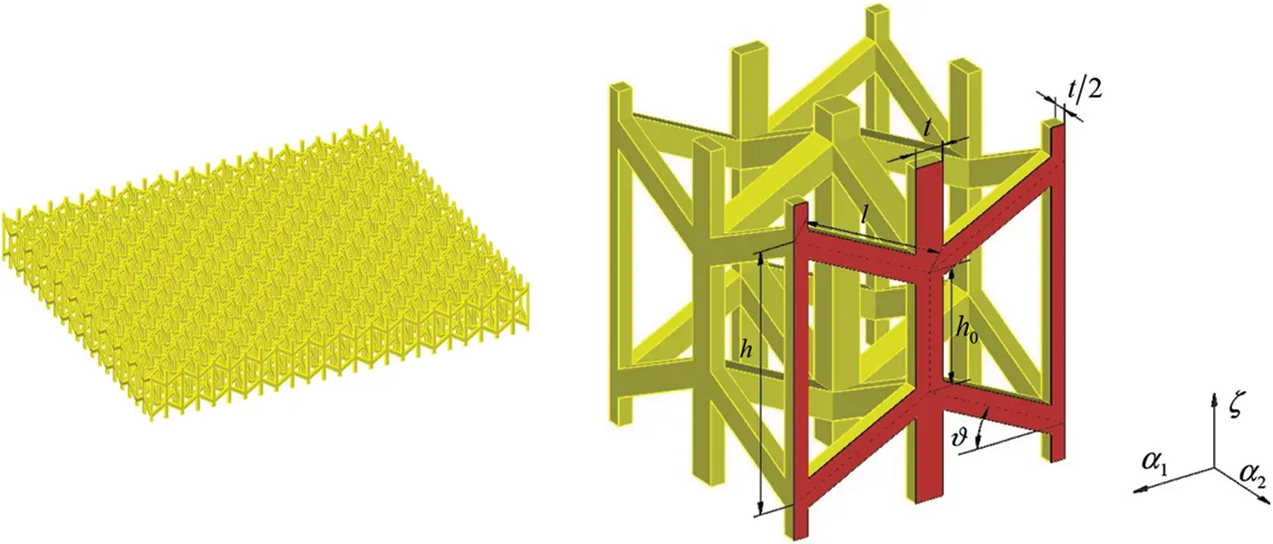
Figure 3: Geometric representation of a 3D Augmented Re-entrant Cellular Structure (3D ARCS) unit cell. The configuration of the 2D unit pattern provides an auxetic behaviour of the equivalent continuum along in-plane directions α1,α2

Starting from reference [109], the classical beam theory is adopted to model each frame, here assumed as thin frame with rigid node area. A preliminary geometric overlapping verification should be performed. The vertical struts do not superimpose to each other if the following geometric relation is respected:

t<lsin⁡ϑ1(146)

being ϑ1=π/π22−ϑ. Moreover, the overlapping test for inclined tips is based on the following inequality:

(1−cos⁡ϑ1)tsin⁡ϑ1+2lcos⁡ϑ1<h¯(147)

The following stiffnesses are conveniently introduced, accounting for the extensional behaviour and the bending deflections of the frame [109]:

k sl=E stβk sh=E stγk sh 0=E stηk fl=E stβ3k fh 0=E stη3k fh=E stγ3(148)

Moreover, the generalized stiffness parameter ϕ is defined as:

ϕ=cos2ϑkfl+sin2ϑksl(149)

Based on the Eqs. (148) and (149), the quantities A,B are defined as:

A=ϕ−1kslϕ+1ksh0+1ksh1ksh0+1ksh2ϕ,B=1kfl−1ksl(150)

Following the procedure in reference [109], the 3D ARCS k-th layer can be homogenized as an orthotropic medium. The correspondent Elastic moduli E1(k),E2(k),E3(k) are expressed as:

E1(k)=E2(k)=2h¯0+h¯11ksl+(A+1ϕksl)B sin2ϑ,E3(k)=h¯0+h¯l2cos2ϑϕksh0ksh+ksh0+kshϕksh0+ϕksh+4(151)

whereas the shear moduli G12(k),G13(k),G23(k) are defined as:

G12(k)=kflh¯0+h¯G13(k)=G23(k)=βcos⁡ϑ11kfh0+kfh4tlcos⁡ϑh¯0+h¯+(tcos⁡ϑ(h¯−lsin⁡ϑ)kfl+kfh−kfh0kfl(kfh+kfh0)tlcos⁡ϑsin⁡ϑ)(1l−sin⁡ϑh¯0+h¯)(152)

In the following, the expressions for Poisson’s orthotropic coefficients ν12(k),ν13(k),ν23(k) can be found:

ν12(k)=−ABsin2ϑ1ksl+(A+1ϕksl)Bsin⁡ϑ,ν13(k)=ν23(k)=−lh¯0+h¯(ϕ−1ksl)(ksh−ksh0)ϕksh0ksh+ksh0+ksh1ksl+(A+1ϕksl)Bsin⁡ϑ(153)

In addition, the homogenized density of the 3D ARCS layer is computed according to the following expression, applying the procedure of void fraction introduced in reference [110]:

ρ(k)=ρs(α+4−3+cos⁡ϑ1sin⁡ϑ1β+2h¯0l)β22sin2ϑ1(α−cos⁡θ)(154)

9.2 Straight Panels

The first set of numerical investigations considers some rectangular plates of constant thickness with general boundary conditions and subjected to a static uniform load. All the mechanic and geometric properties of the structure are reported in Fig. 4. A convergence study starts considering a fully clamped rectangular plate of dimensions Lx=1.5m and Lx=1m subjected to uniform pressure q3a(+)=−1.0×104Pa. The lamination scheme accounts for two external triclinic layers and a central orthotropic lamina made of graphite-epoxy. A reference 3D FEM solution has been provided, and the vertical deflection of the central part of the structure has been computed. The results are summarized in Table 1, with a clear fast convergence for all the displacement field assumptions.

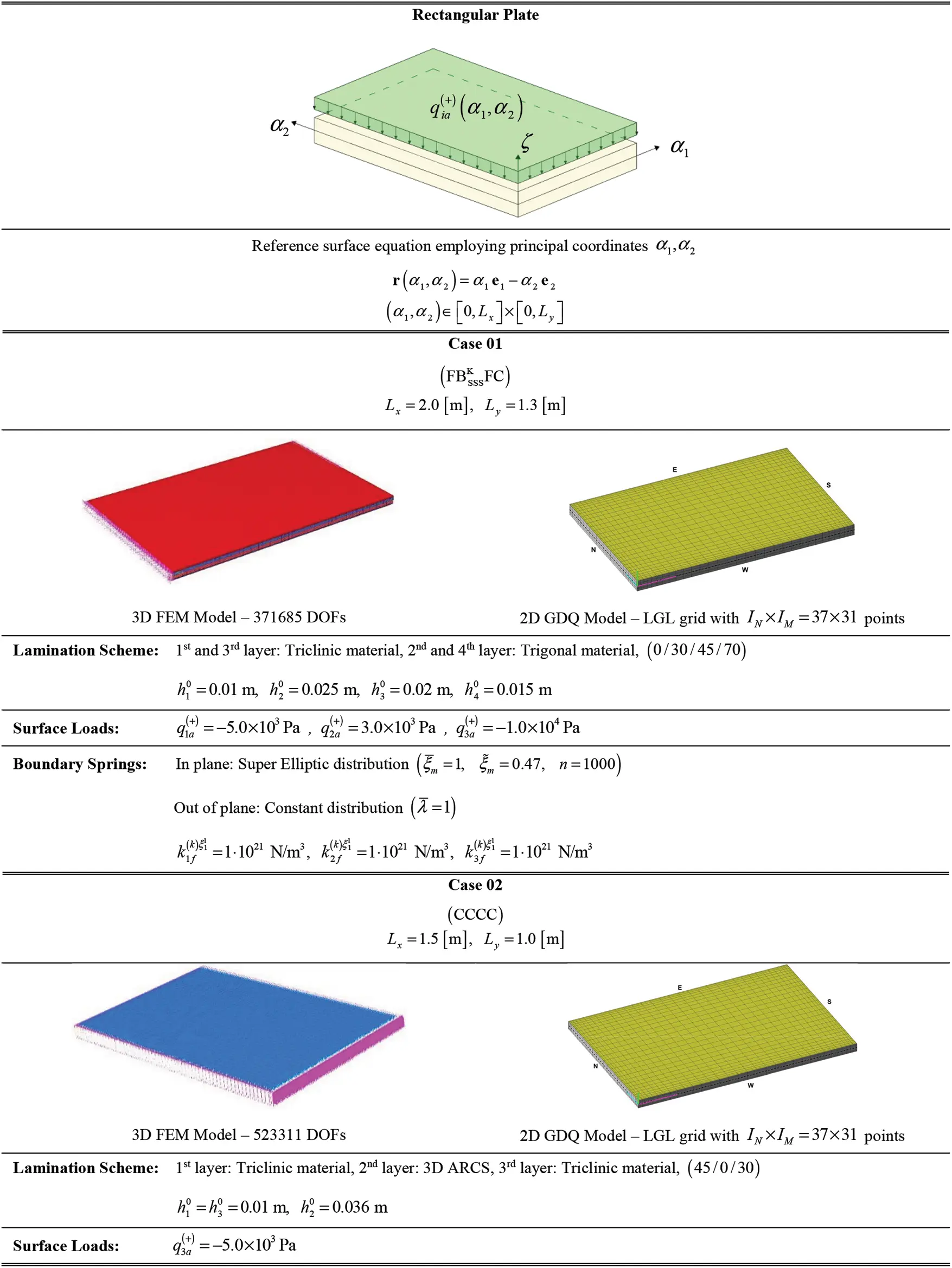
Figure 4: Geometric and mechanical properties for an anisotropic rectangular plate enforced with non-conventional boundary conditions and subjected to a general loading

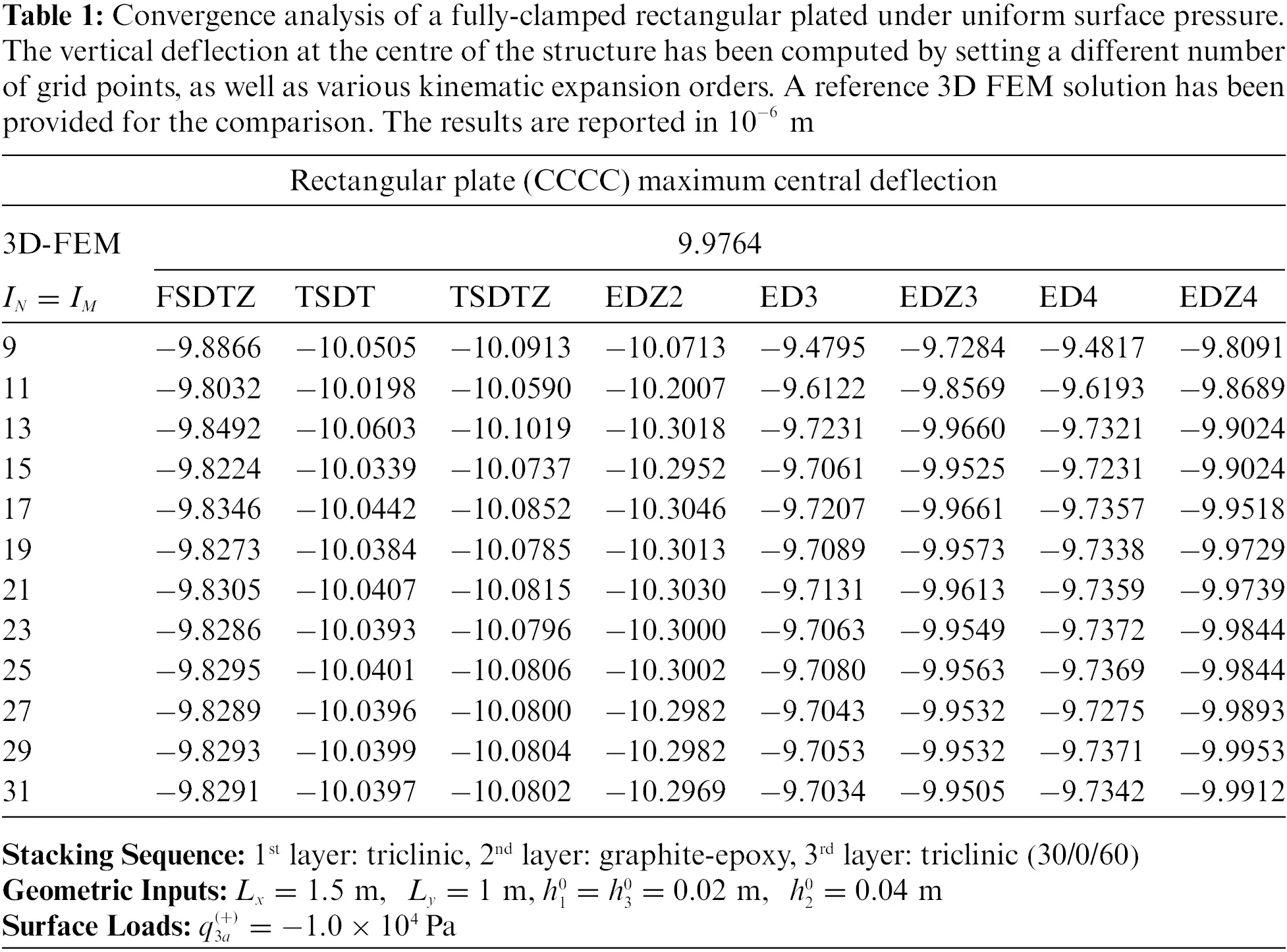
In particular, two different configurations have been considered. For the Case 01, four layers with general orientations (0/30/45/70) have been employed in the lamination scheme, embedding the triclinic material of Eq. (142) and the trigonal material introduced in Eq. (143). As far as the external constraints is concerned, the super elliptic distribution of Eq. (77) has been employed, leading to a half edge clamped condition. A general uniform pressure q~(α1,α2)=1 has been applied on the top surface of the shell, characterized by both normal q3a(+) and tangential components q1a(+),q2a(+) with respect to α1,α2,ζ principal directions. A reference solution has been computed with a 3D FEM model, employing 371685 DOFs. The GDQ simulations, instead, were performed on a computational grid based on the LGL distribution of Eq. (100) characterized by IN=37 and IM=31. Different higher order theories have been considered according to Eq. (27), together with the zigzag effects. The static structural response has been reported in Figs. 5–7. The 3D displacement field components U1,U2,U3 through-the-thickness distributions of Fig. 5 taken from the point located in the centre of the structure show that an almost linear distribution of in-plane components is predicted with all the assumptions, whereas a constant dispersion of U3 is assumed.

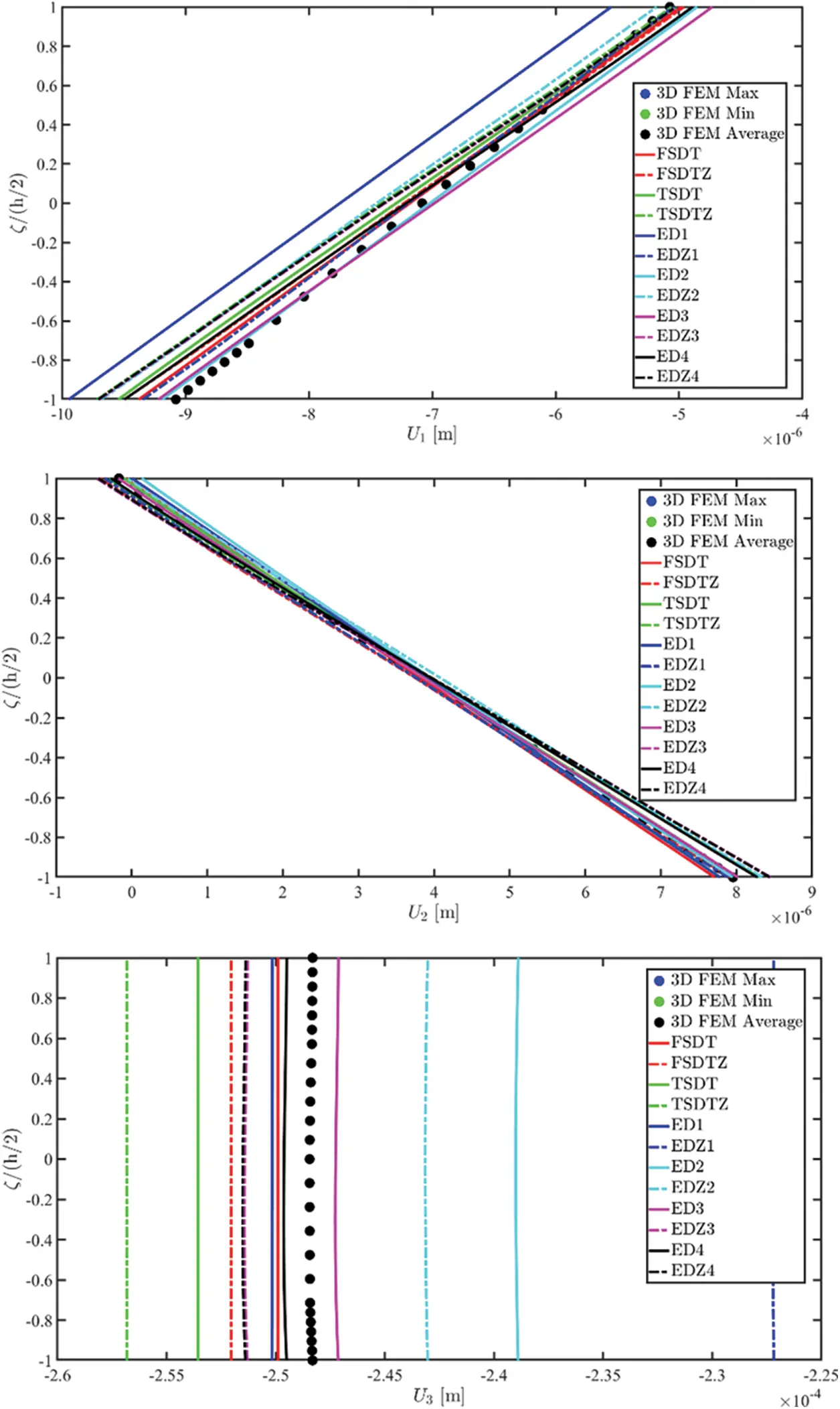
Figure 5: Through-the-thickness distributions at (0.50(ξ11−ξ10),0.50(ξ21−ξ20)) of the three-dimensional displacement field vector U(α1,α2,ζ) of a rectangular plate composed of four generally anisotropic layers under static loads (q~3(+)=−10000Pa) enforced with general boundary conditions (FBSSSKFC)

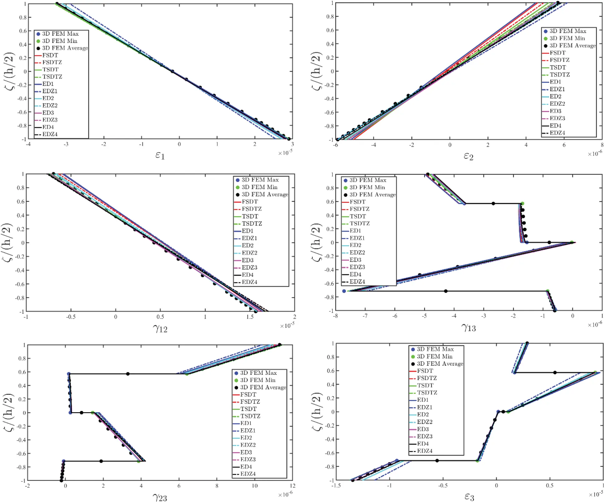
Figure 6: Through-the-thickness distributions at (0.50(ξ11−ξ10),0.50(ξ21−ξ20)) of the three-dimensional strain vector ε(α1,α2,ζ) of a rectangular plate composed of four generally anisotropic layers under static loads (q~3(+)=−10000Pa) enforced with general boundary conditions (FBSSSKFC)

On the other hand, the best agreement with the 3D FEM outcomes is provided by the EDZ4 theory for all the components. As far as the 3D strain vector dispersions are concerned (Fig. 6), the GDQ approach predicts well the kinematic variables. In this case, the simulation with a fourth kinematic expansion order without the zigzag effect (ED4) seems to be more accurate, even though all the approaches provide very good results. The employment of a higher order assumption for the displacement field is crucial for the γ13 distortion component, since in the third layer the 3D FEM predicts a slight nonlinear dispersion. The through-the-thickness distributions of stresses reported in Fig. 7 employing the EDZ4 higher order assumption of the displacement field are perfectly in line with those belonging to the 3D reference solution. It can be seen that lower order ED1 and EDZ1 shell theories cannot give results of the same accuracy, even when embedding a zigzag function within the formulation.

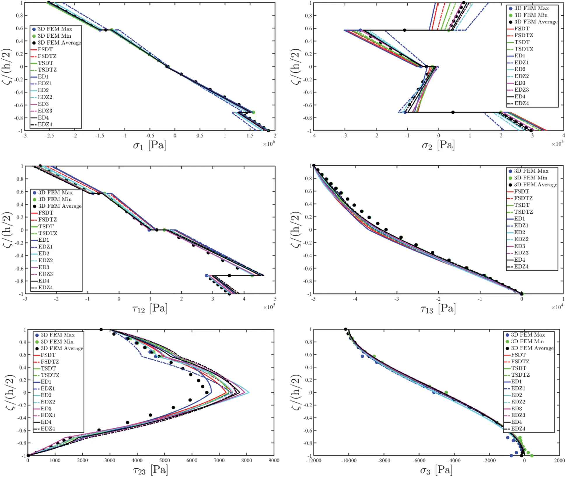
Figure 7: Through-the-thickness distributions at (0.50(ξ11−ξ10),0.50(ξ21−ξ20)) of the three-dimensional stress vector σ(α1,α2,ζ) of a rectangular plate composed of four generally anisotropic layers under static loads (q~3(+)=−10000Pa) enforced with general boundary conditions (FBSSSKFC)

The second investigation was performed on a fully-clamped (CCCC) rectangular plate under a uniform static pressure along the ζ coordinate. The structure is characterized by two external layers of the triclinic material assessed in Eq. (142) and a central core made of an orthotropic 3D ARCS, whose mechanical properties are computed employing the homogenization provided by Eqs. (151)–(154). In particular, the geometric input quantities have been selected so that h¯=0.0024m, h¯0=l=0.0012m and ϑ=π/π66. The tips and struts thicknesses are chosen so that t=0.05l. The constitutive material is intended to be isotropic with an elastic modulus Es=196GPa and a density equal to ρs=7800kg/kgm3m3. The central isotropic layer is obtained from a superimposition of five cells. Thickness plots have been derived at (0.25(ξ11−ξ10),0.25(ξ21−ξ20)), and they have been reported in Figs. 8–10. In this case, since the central layer behaves like a softcore, two different stable reference solutions have been computed, namely the 3D FEM and a fourth-order Layer-Wise (LD4) calculated by means of the GDQ method [19]. For the sake of completeness, the simulation has been performed also with the EDZ4 displacement field theory, employing the strong formulation [27]. Fig. 8 shows that the employment of higher order theories, together with the zigzag assumption, is required for seeking results in line with other theories for both in-plane and out-of-plane displacement field components. This is due to the fact that the central softcore layer of 3D ARCS induces an unconventional in-plane deflection of the structure due to the static pressure. Similar considerations can be made for the 3D strain components of Fig. 9. Note that both the 3D FEM and LD4 predict a behaviour typical of lamination schemes embedding softcore layers. Also for this case, the zigzag effect is very evident, since common ED−N theories are not adequate. Referring to out-of-plane distortions γ13 and γ23, the squeezing effect of the central core of the plate is outlined. Actually, the ESL simulations not including the zigzag axiomatic assumption of Eq. (27) are not capable of predicting the right structural response. The EDZ3 solution is in line with LD4 and 3D FEM predictions for all strain components. Also for the stress component vector through-the-thickness dispersions reported in Fig. 10, the employment of the zigzag function leads to good predictions in line with reference simulations, regardless the kinematic expansion order. In the case of σ3(k) three-dimensional stress component, higher order theories provide results in line with the 3D FEM outcomes. Lower order theories account only for the fulfilment of the external loads, because of the recovery algorithm assessed in Eq. (137).

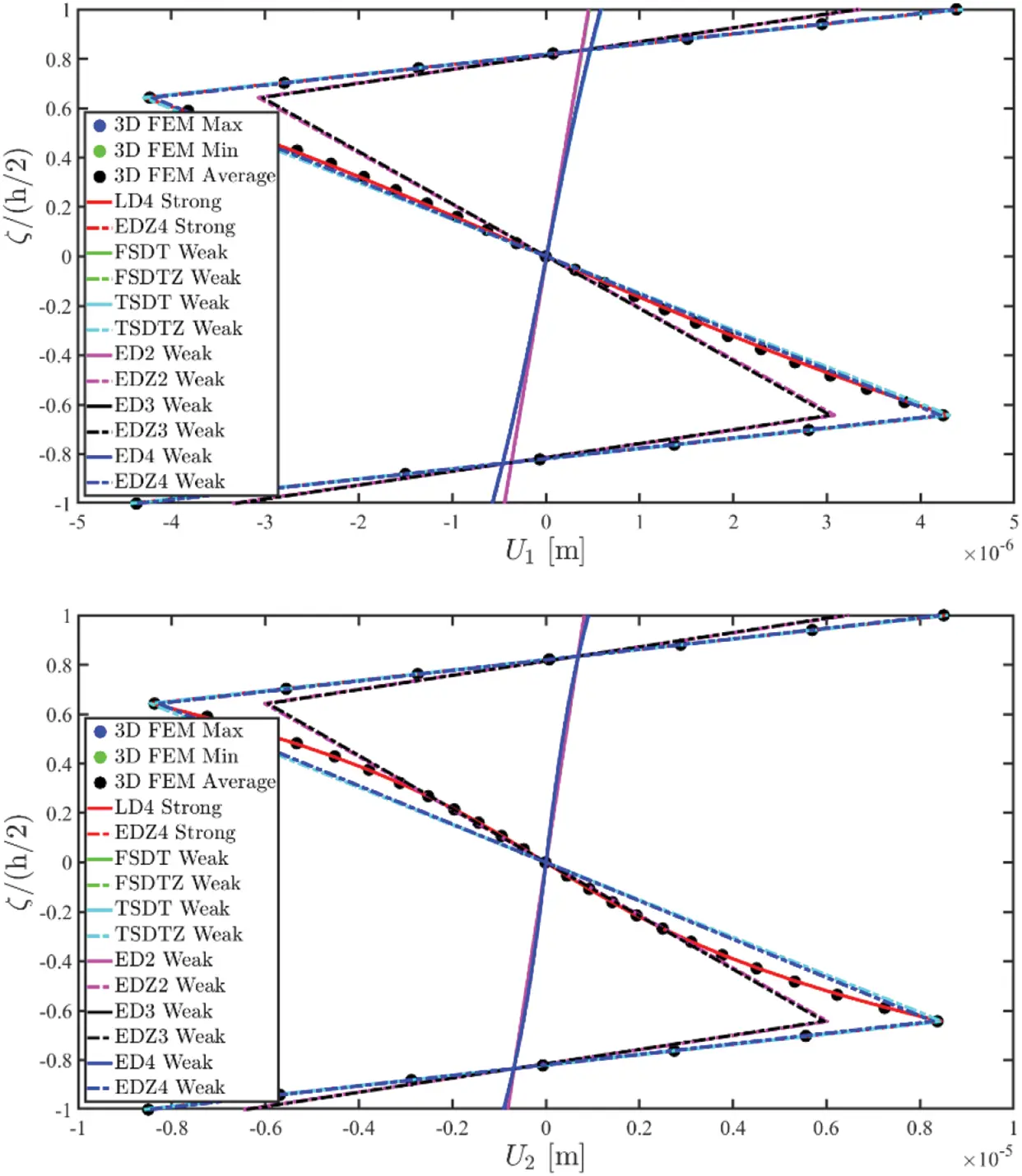
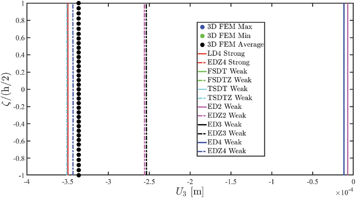
Figure 8: Through-the-thickness distributions at (0.25(ξ11−ξ10),0.25(ξ21−ξ20)) of the three-dimensional displacement field vector U(α1,α2,ζ) of a fully-clamped (CCCC) rectangular plate composed of three generally anisotropic layers under static loads (q~3(+)=−5000Pa) enforced with general boundary conditions (FBSSSKFC)

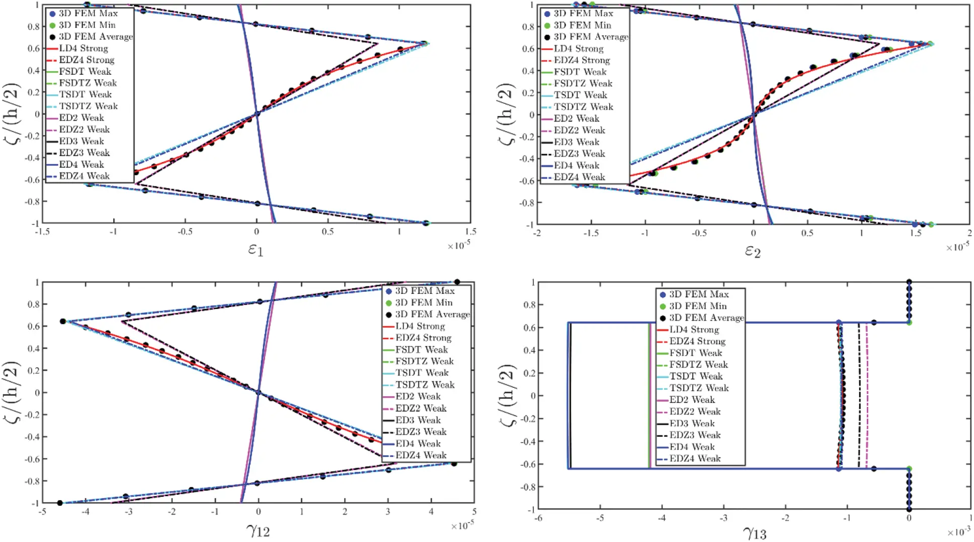
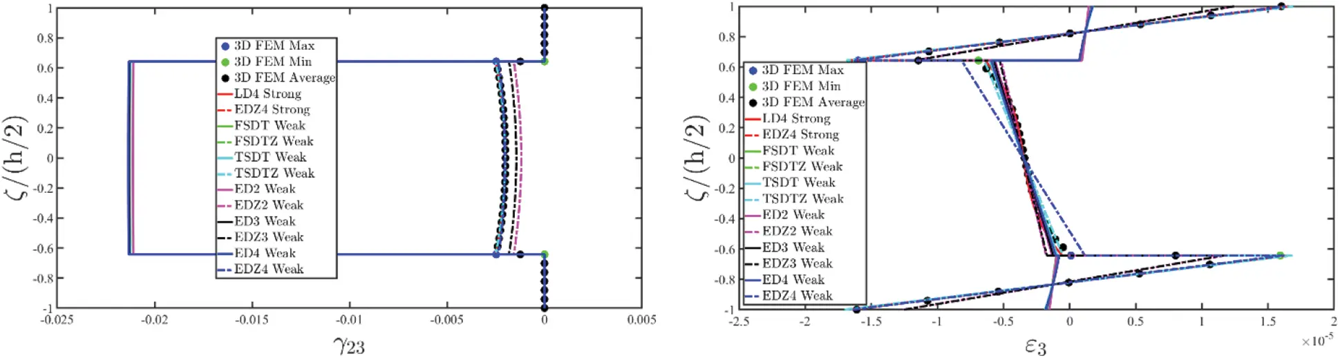
Figure 9: Through-the-thickness distributions at (0.25(ξ11−ξ10),0.25(ξ21−ξ20)) of the three-dimensional strain vector ε(α1,α2,ζ) of a fully-clamped (CCCC) rectangular plate composed of three generally anisotropic layers under static loads (q~3(+)=−5000Pa) enforced with general boundary conditions (FBSSSKFC)

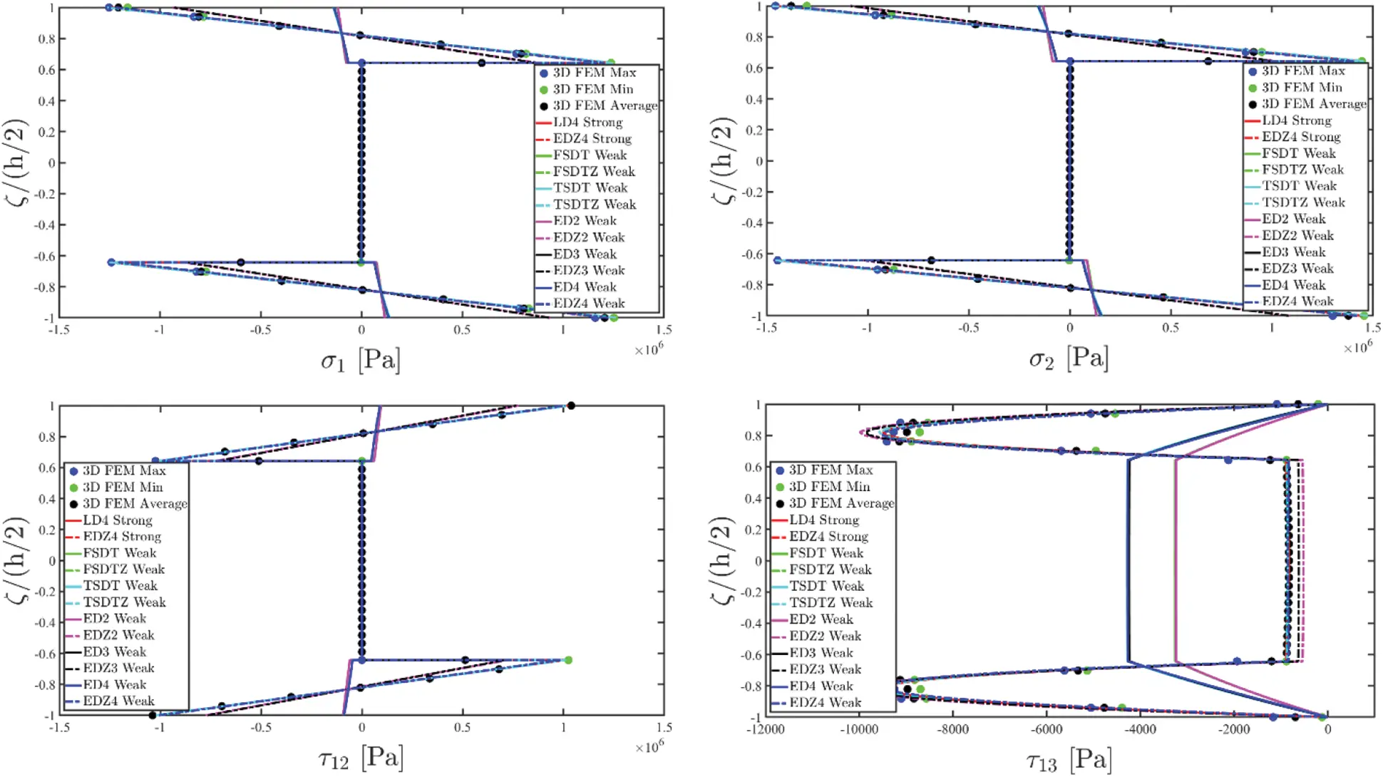
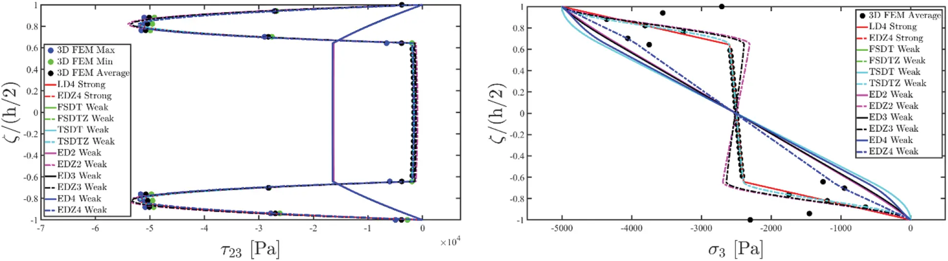
Figure 10: Through-the-thickness distributions at (0.25(ξ11−ξ10),0.25(ξ21−ξ20)) of the three-dimensional stress vector σ(α1,α2,ζ) of a fully-clamped (CCCC) rectangular plate composed of three generally anisotropic layers under static loads (q~3(+)=−5000Pa) enforced with general boundary conditions (FBSSSKFC)

9.3 Panels with Curvatures

In the present section the linear static analysis is performed for laminated structures characterized by the presence of curvature. Accordingly, a singly-curved shell and two doubly-curved panels have been considered, each of them enforced with generalized external constraints. The lamination schemes account for layers characterized by a general orientation with respect to the curvilinear principal reference system. As far as surface pressures are concerned, various loading conditions have been considered. They have been modelled within the ESL framework employing the distributions q¯(α1,α2) outlined in Eqs. (65)–(67).

In Fig. 11, there are all the information regarding the analysed cylindrical panel. According to the ESL approach, the shape of the structure is described starting from the reference surface, as shown in Eq. (2). In the following, the expression of the reference surface is reported employing principal curvilinear coordinates α1,α2, setting Rb the radius of the circle [16]:

r(α1,α2)=Rbcos⁡α2e1−Rbsin⁡α2e2+α1e3(155)

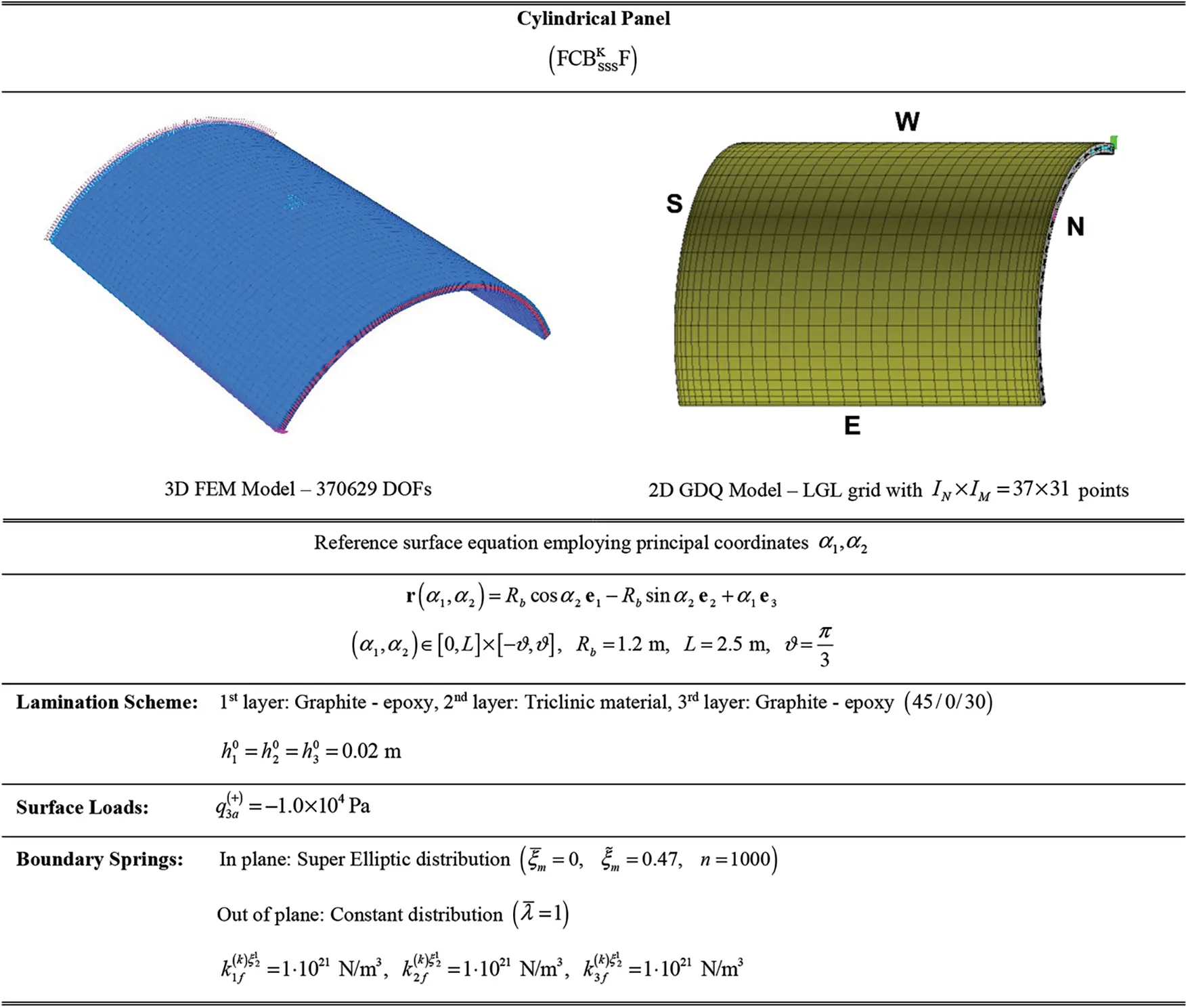
Figure 11: Geometric and mechanical properties for an anisotropic cylindrical panel enforced with non-conventional boundary conditions and subjected to general loads

The stacking sequence accounts for three layers. Namely, a central triclinic material has been covered by two external sheets of graphite-epoxy of the same thickness. A uniform surface load q3a(+)=−1.0⋅104Pa has been applied to the top surface (ζ=+h/h22) of the shell. Boundary conditions account for the clamping of the South (S) edge, whereas the East (E) side is constrained in a portion of its length by means of the super elliptic distribution described in Eq. (77). The structural response has been outlined in Figs. 12–14 which refer to the dispersions of kinematic and static quantities along with the shell thickness in the region located at the centre of the physical domain. 3D displacement field components U1,U2,U3 have been reported in Fig. 12. It is shown that the 3D FEM solution is properly predicted by the higher order models, especially for the out-of-plane component which cannot be predicted by lower order assumptions like the ED1 displacement field. The in-plane components are characterized by a linear distribution instead. On the other hand, an excellent agreement between different ESL approaches can be found in Fig. 13, regardless of the employment of the zigzag function. Also, for this case, ED1 predictions are not in line with the outcomes from refined 3D FEM. As can be seen from Fig. 14, also the 3D stress component vectors coming from different ESL approaches are in line with those obtained from the commercial software. Referring to the τ13,τ23 and σ3 dispersions, the exact fulfilment of the external load conditions can be easily seen. The worst accuracy is obtained when N=1.

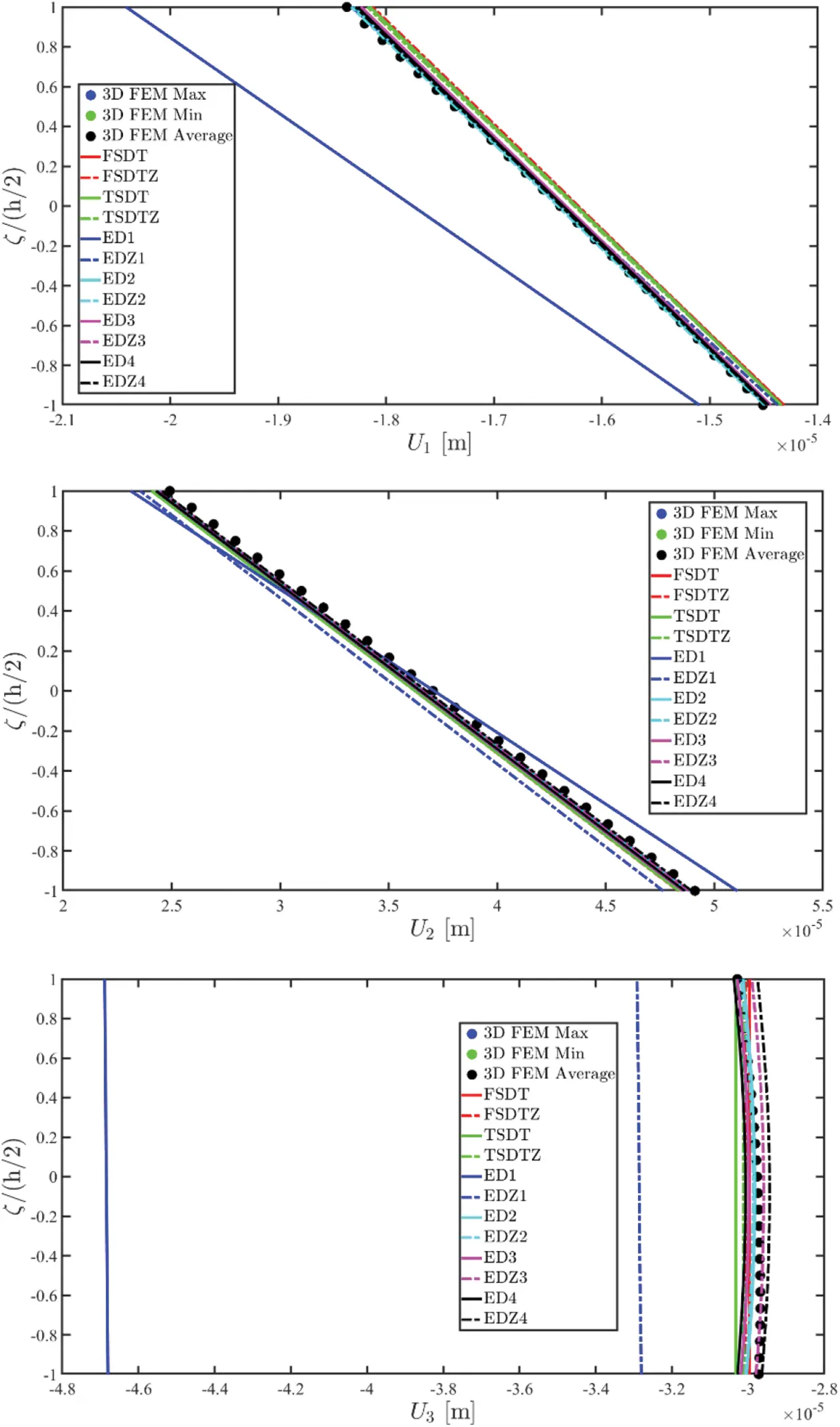
Figure 12: Through-the-thickness distributions at (0.50(ξ11−ξ10),0.50(ξ21−ξ20)) of the three-dimensional displacement field vector U(α1,α2,ζ) of a cylindrical panel composed of three generally anisotropic layers under static loads (q~3(+)=−10000Pa) enforced with general boundary conditions (FCBSSSKF)

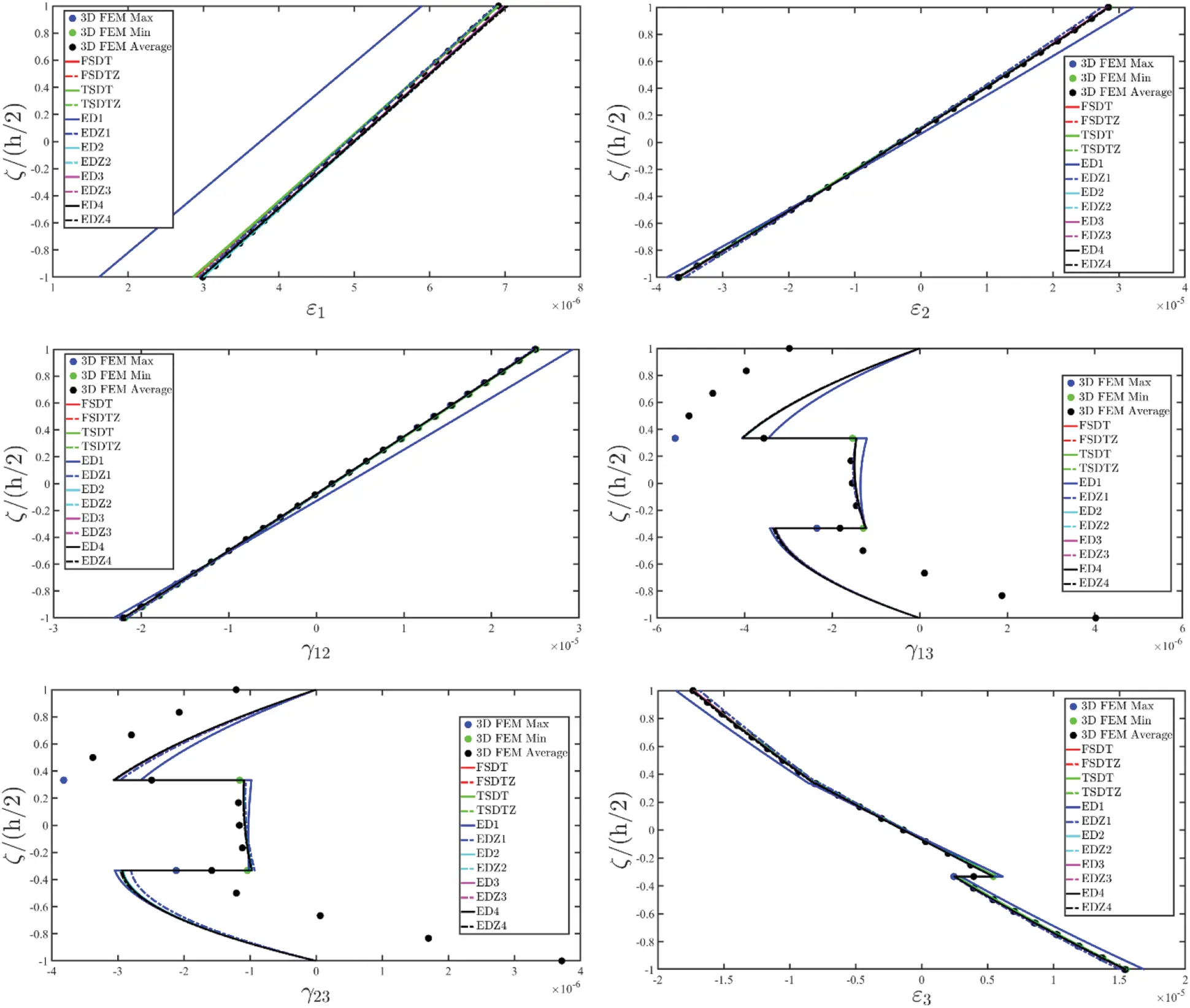
Figure 13: Through-the-thickness distributions at (0.50(ξ11−ξ10),0.50(ξ21−ξ20)) of the three-dimensional strain vector ε(α1,α2,ζ) of a cylindrical panel composed of three generally anisotropic layers under static loads (q~3(+)=−10000Pa) enforced with general boundary conditions (FCBSSSKF)

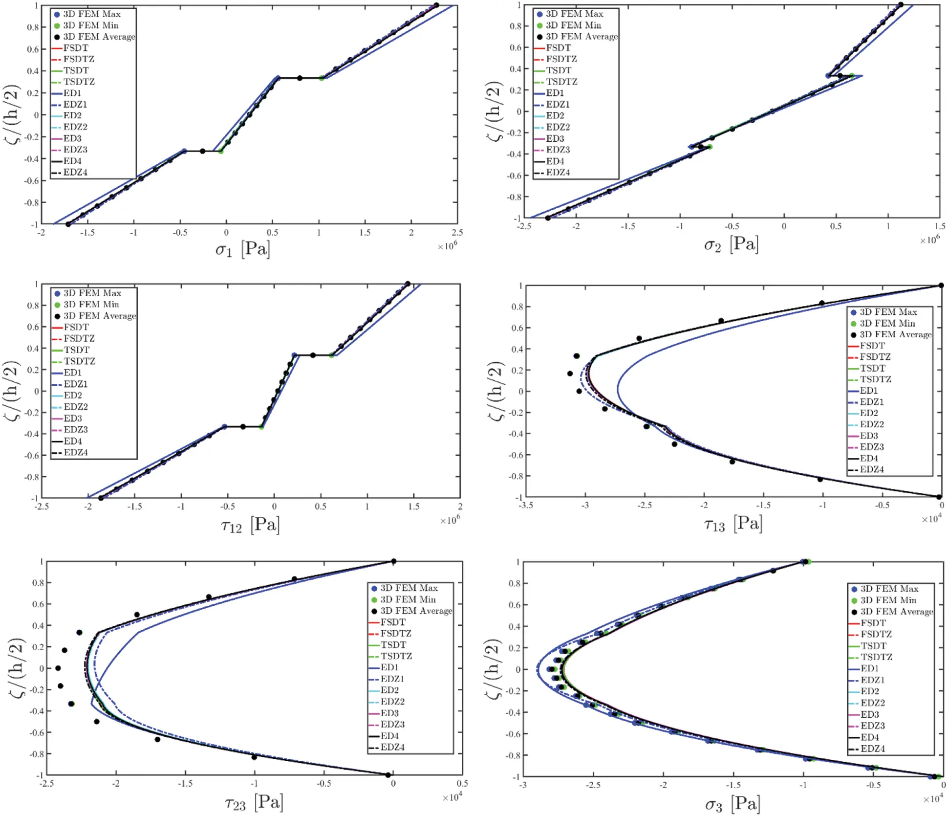
Figure 14: Through-the-thickness distributions at (0.50(ξ11−ξ10),0.50(ξ21−ξ20)) of the three-dimensional stress vector σ(α1,α2,ζ) of a cylindrical panel composed of three generally anisotropic layers under static loads (q~3(+)=−10000Pa) enforced with general boundary conditions (FCBSSSKF)

Next numerical investigation is performed on a doubly-curved panel of translation of mapped geometry. In particular, a hyperbolic paraboloid has been considered, whose reference surface equation in principal coordinates is reported [16]:

r(α 1,α2)=(12kα 1tanα 1+14kα 2tan2 α 2sinα 1)  e1+(−12kα 2tan2α 2) e2                      +(14kα 1tan2 α 1+14kα 2tan2 α2cosα 1)e3(156)

being kα1,kα2 two characteristic parameters depending on the curvature of the principal lines. A geometric representation of the structure at issue is reported in Fig. 15, together with all the lamination scheme information and the boundary conditions. The physical domain mapping has been assessed by means of the NURBS-based procedure of Eq. (13) with all the information related to each surface edge reported in Fig. 15. External constraints have been modelled on the structure setting the West (W) side fully clamped. The employment of the Double–Weibull distribution defined in Eq. (78) accounts for the perfect clamping of the two external points of the East (E) edge. A uniform load has been applied in a quarter of the structure on the top surface. Within the GDQ simulation, such discrete variation of the load has been modelled by means of the Super Elliptic distribution reported in Eq. (67). In the out-of-plane direction, linear elastic springs follows a uniform dispersion (λ¯(ζ)=1). In Fig. 16, the dispersion of the displacement field components U1,U2,U3 at (0.50(ξ11−ξ10),0.50(ξ21−ξ20)) are collected coming from various higher order theories. The refined 3D FEM outcomes are taken as references. It is shown that the U1 deflection is well predicted by the proposed formulation with a higher order assumption of the displacement field. On the other hand, other in-plane field variable is not well predicted. As far as the vertical deflection is concerned, the structure at issue is characterized by a certain stretching along with the shell thickness. The shape of the distribution is depicted as well. The three-dimensional strain components are collected in Fig. 17. It is shown that the 3D FEM solution can be fit by higher order assumptions of the displacement field together with the zigzag function. In particular, best performances are provided by the EDZ4 solution. The same considerations can be repeated for the three-dimensional stress vector σ(α1,α2,ζ) of Fig. 18. In fact, the shape of the distributions is well predicted by all the proposed theories. It is interesting to note that the implemented recovery algorithm leads to the perfect fulfilment of the equilibrium boundary conditions coming from external surface loads.

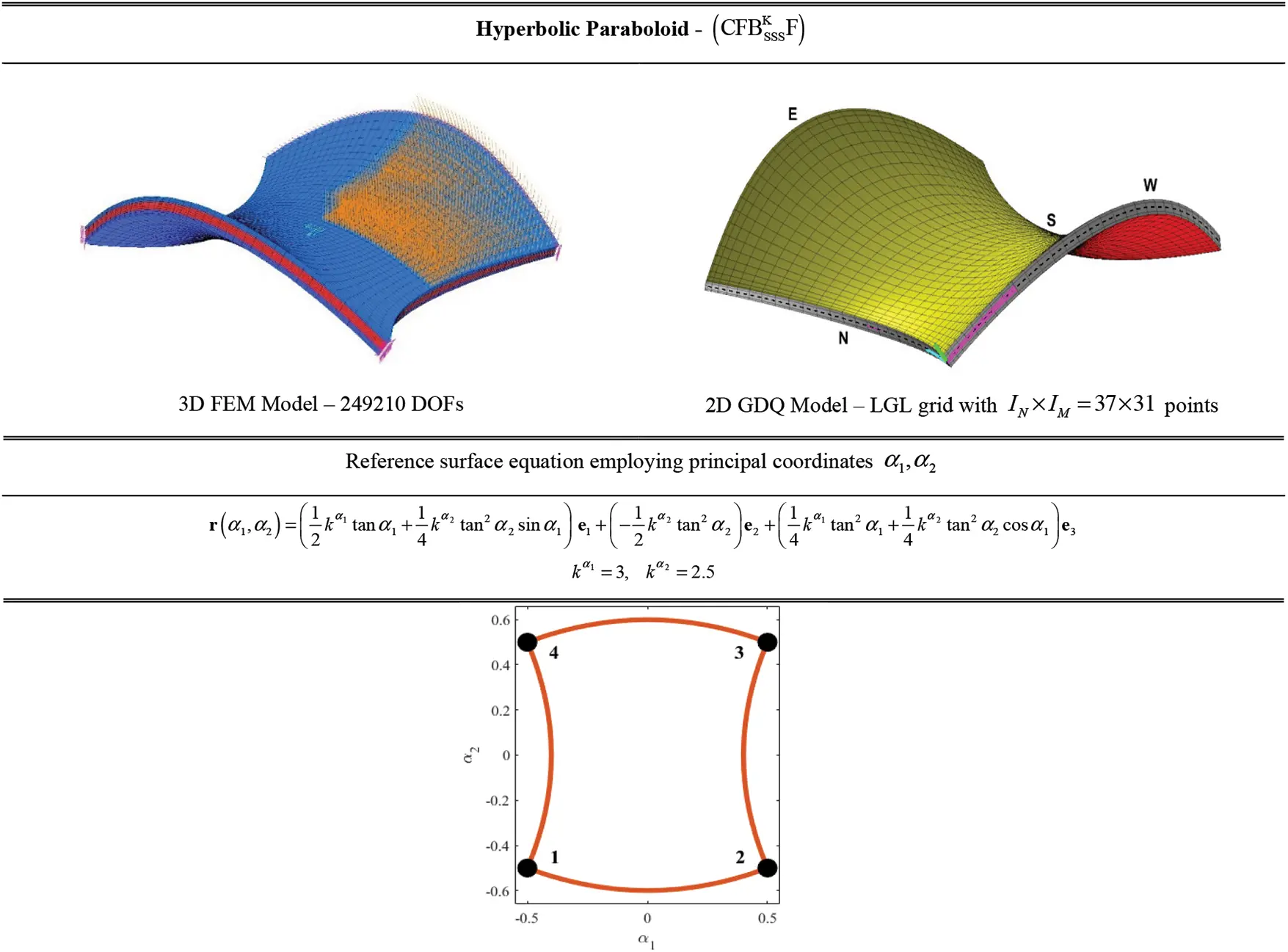
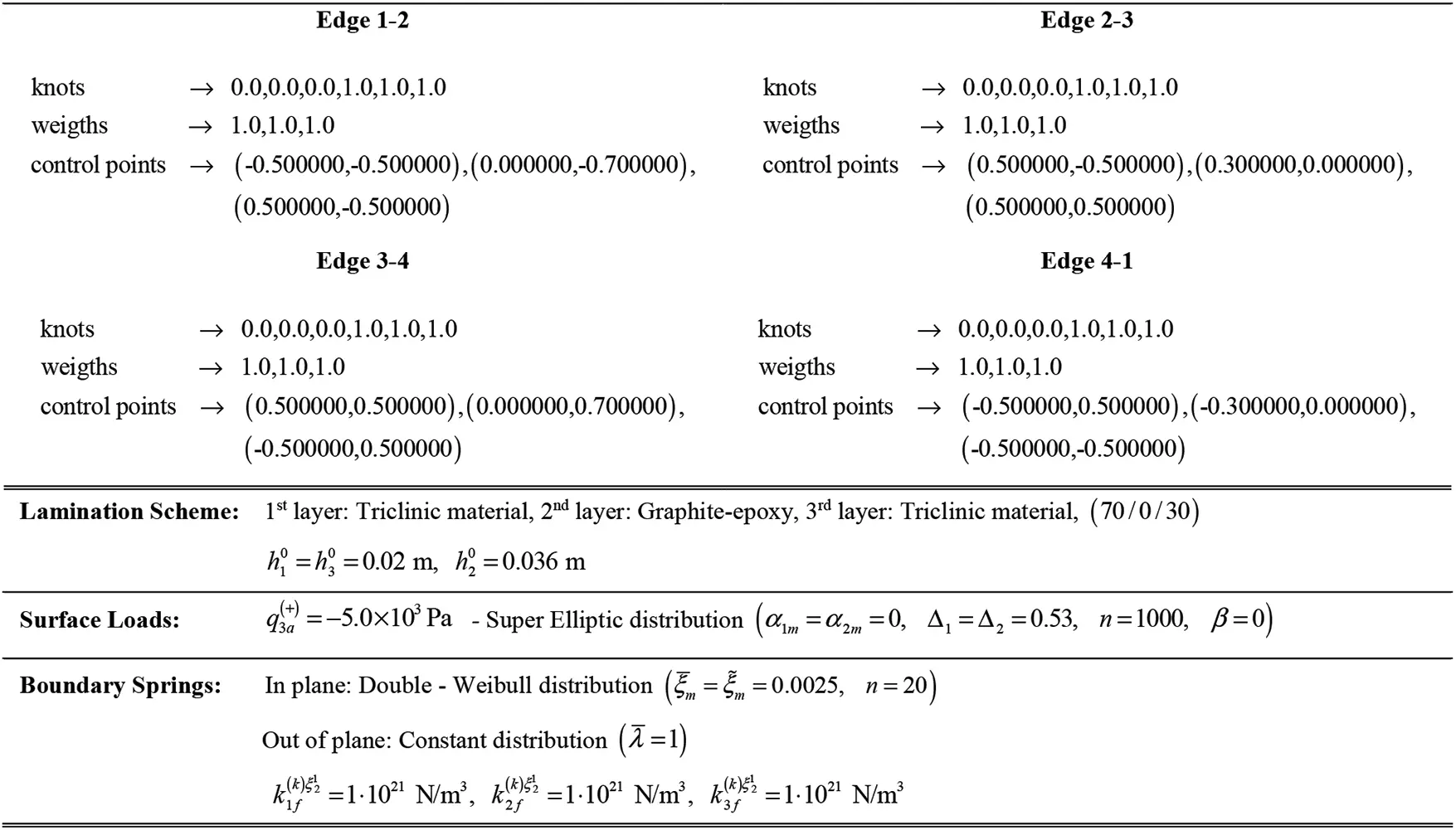
Figure 15: Geometric and mechanical properties of an anisotropic mapped Hyperbolic Paraboloid enforced with non-conventional boundary conditions and subjected to general loads

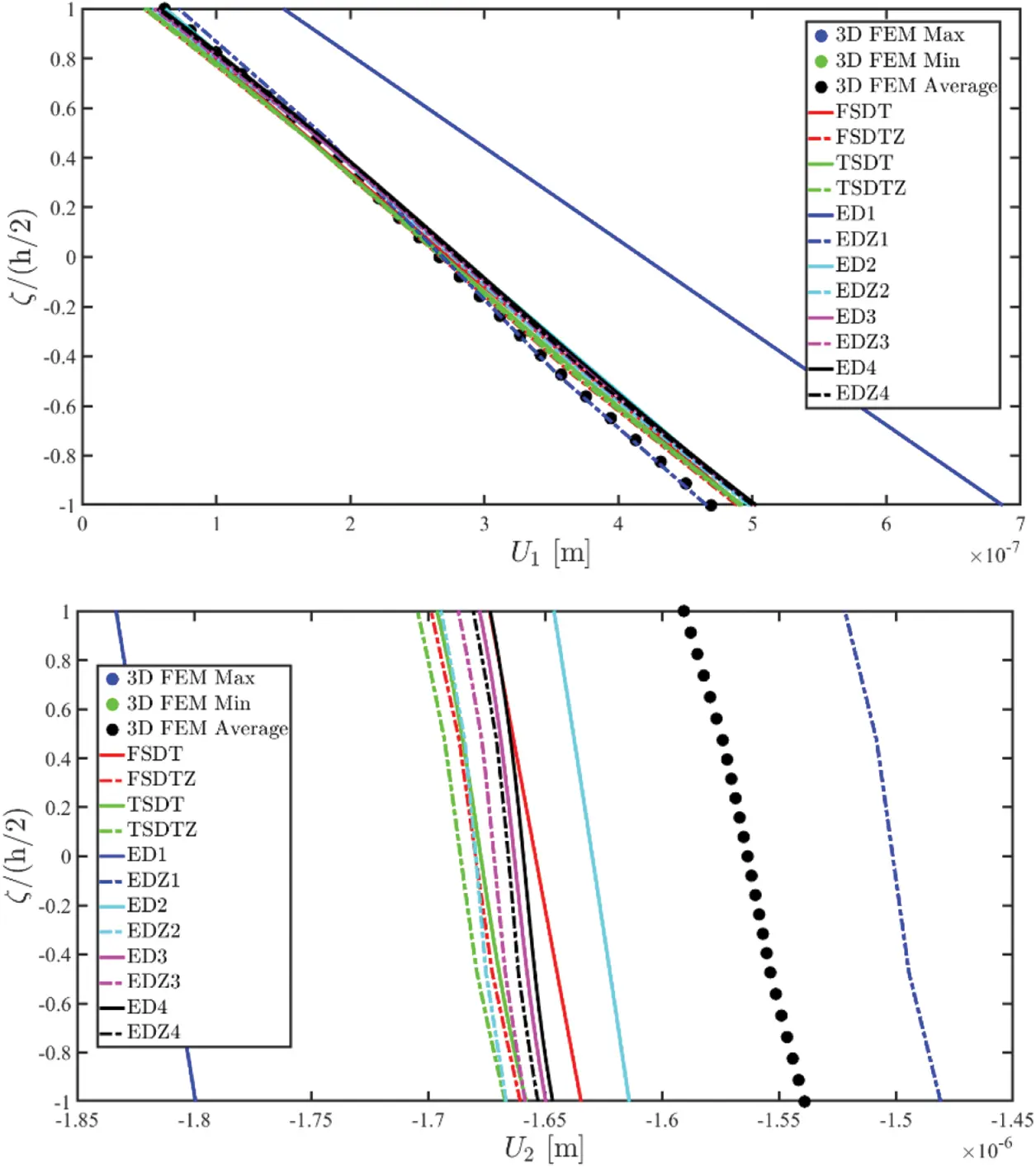
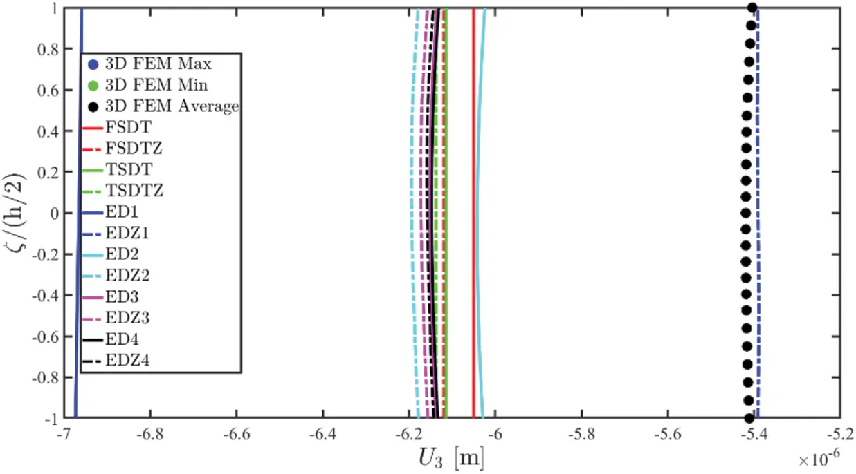
Figure 16: Through-the-thickness distributions at (0.50(ξ11−ξ10),0.50(ξ21−ξ20)) of the three-dimensional displacement field vector U(α1,α2,ζ) of a hyperbolic paraboloid of arbitrary shape composed of three generally anisotropic layers under static loads (q~3(+)=−5000Pa) enforced with general boundary conditions (CFBDDDKF)

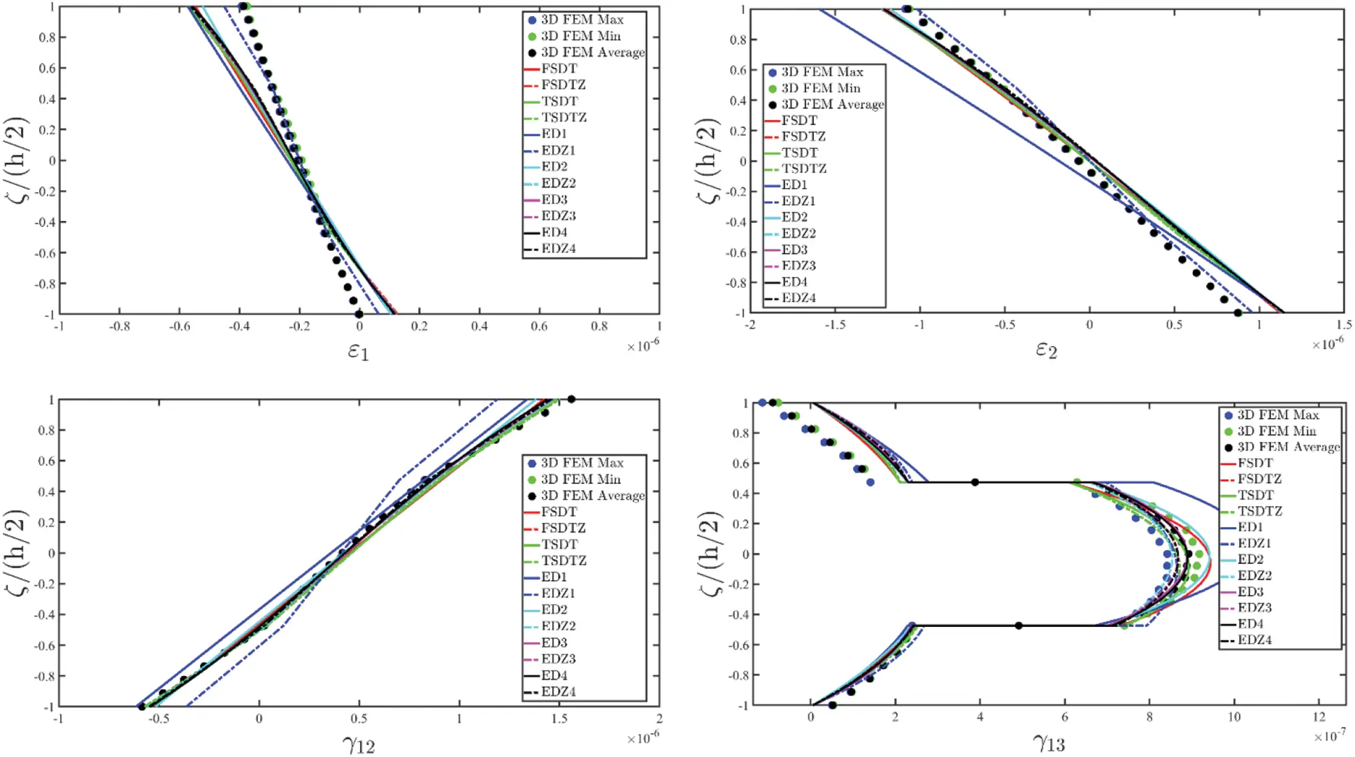
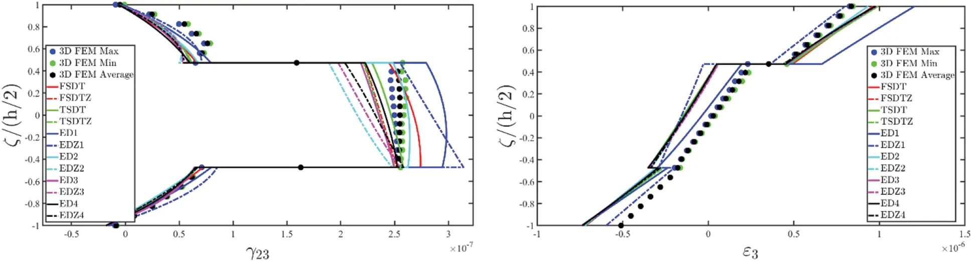
Figure 17: Through-the-thickness distributions at (0.50(ξ11−ξ10),0.50(ξ21−ξ20)) of the three-dimensional strain vector ε(α1,α2,ζ) of a hyperbolic paraboloid of arbitrary shape composed of three generally anisotropic layers under static loads (q~3(+)=−5000Pa) enforced with general boundary conditions (CFBDDDKF)

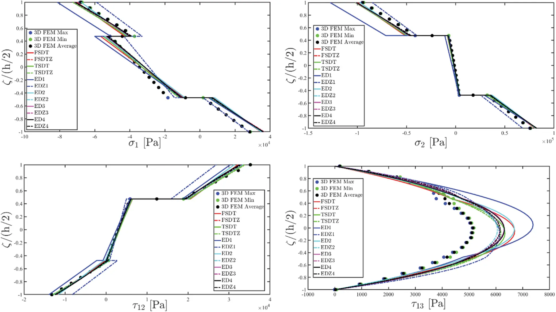
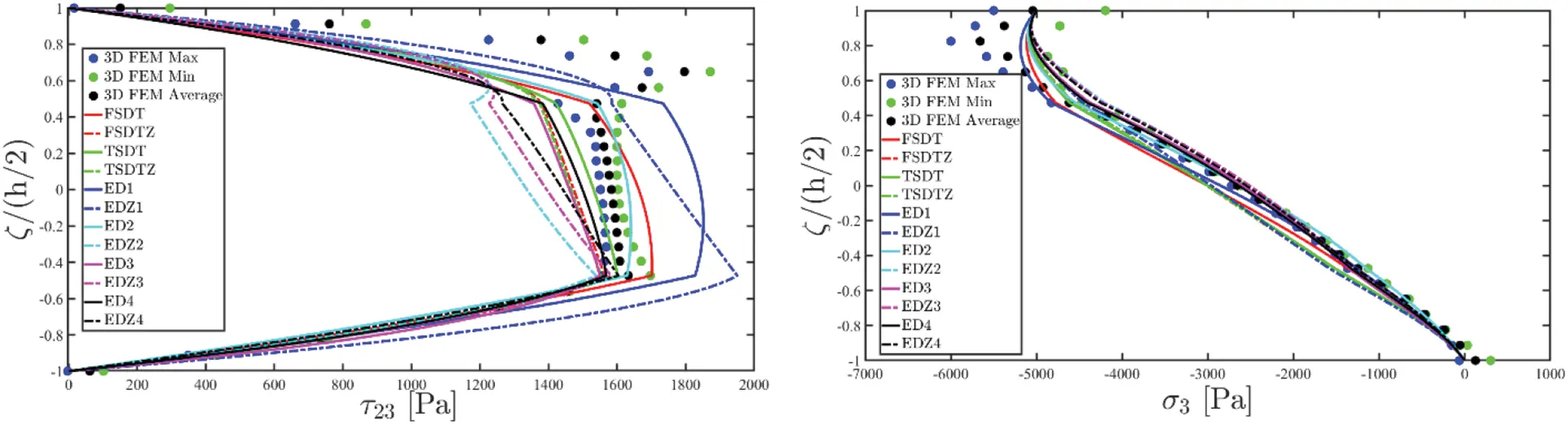
Figure 18: Through-the-thickness distributions at (0.50(ξ11−ξ10),0.50(ξ21−ξ20)) of the three-dimensional stress vector σ(α1,α2,ζ) of a hyperbolic paraboloid of arbitrary shape composed of three generally anisotropic layers under static loads (q~3(+)=−5000Pa) enforced with general boundary conditions (CFBDDDKF)

The last numerical investigation has been performed on a super elliptic panel of revolution enforced with general external constraints along the West (W) mapped edge. Since the shell at issue is a doubly-curved revolution panel, the reference surface equation is computed starting from the general relation based on spherical coordinates [16]:

r(α1,α2)=(R0(α1)cos⁡α2)e1−(R0(α1)sin⁡α2)e2+x3(α2)e3(157)

where R0(α1) denotes the radius of the parallel, whereas x3(α2) is valuated in terms of α2:

R0(α1)=a1a2cos⁡α1(a2n|cos⁡α1|n+a1n|sin⁡α1|n)1n,x3(α2)=−a1a2sin⁡α1(a2n|cos⁡α1|n+a1n|sin⁡α1|n)1n(158)

In Eq. (158), a1,a2 are two geometric characteristic parameters, whereas n denotes the order of the meridian curve. In Fig. 19 a representation of the domain distortion has been provided, together with the knot vector, the weights and the control points coordinate alongside the physical domain.

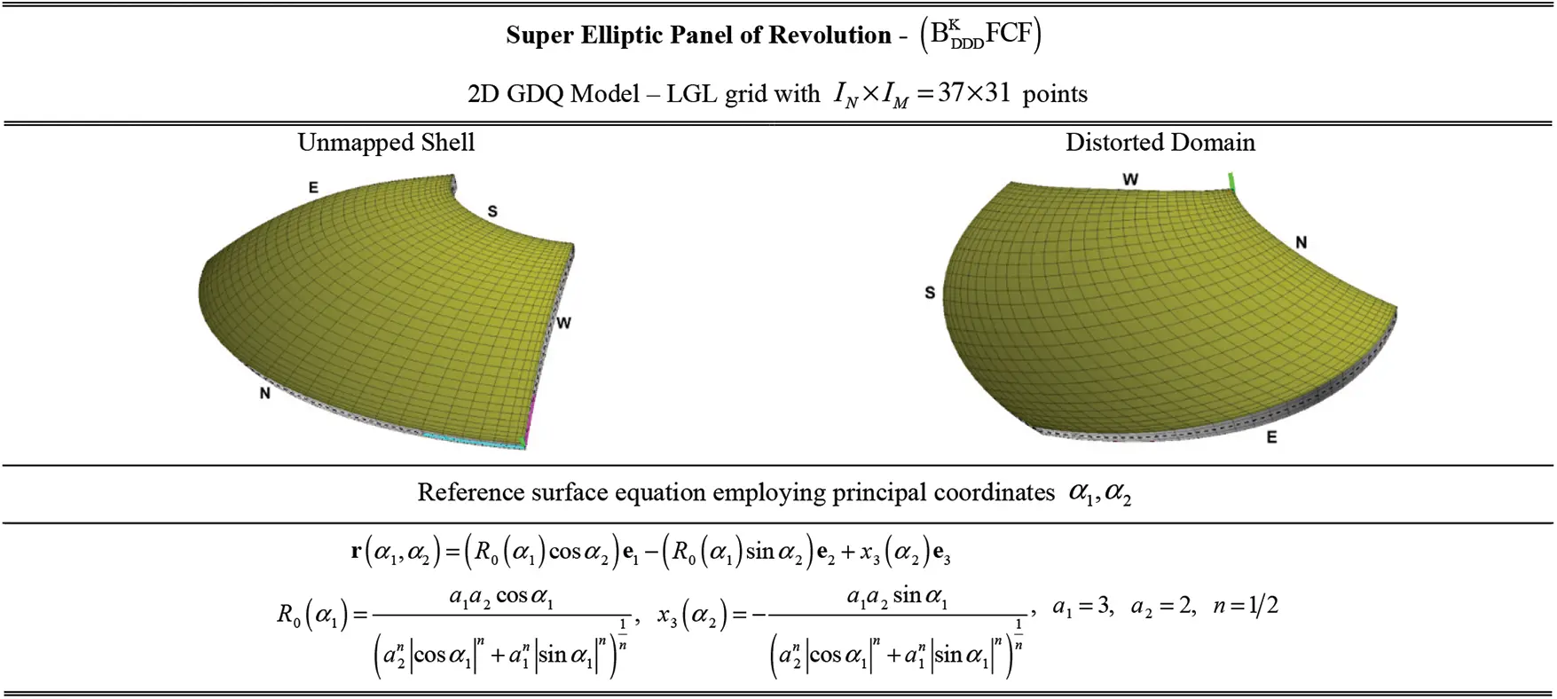
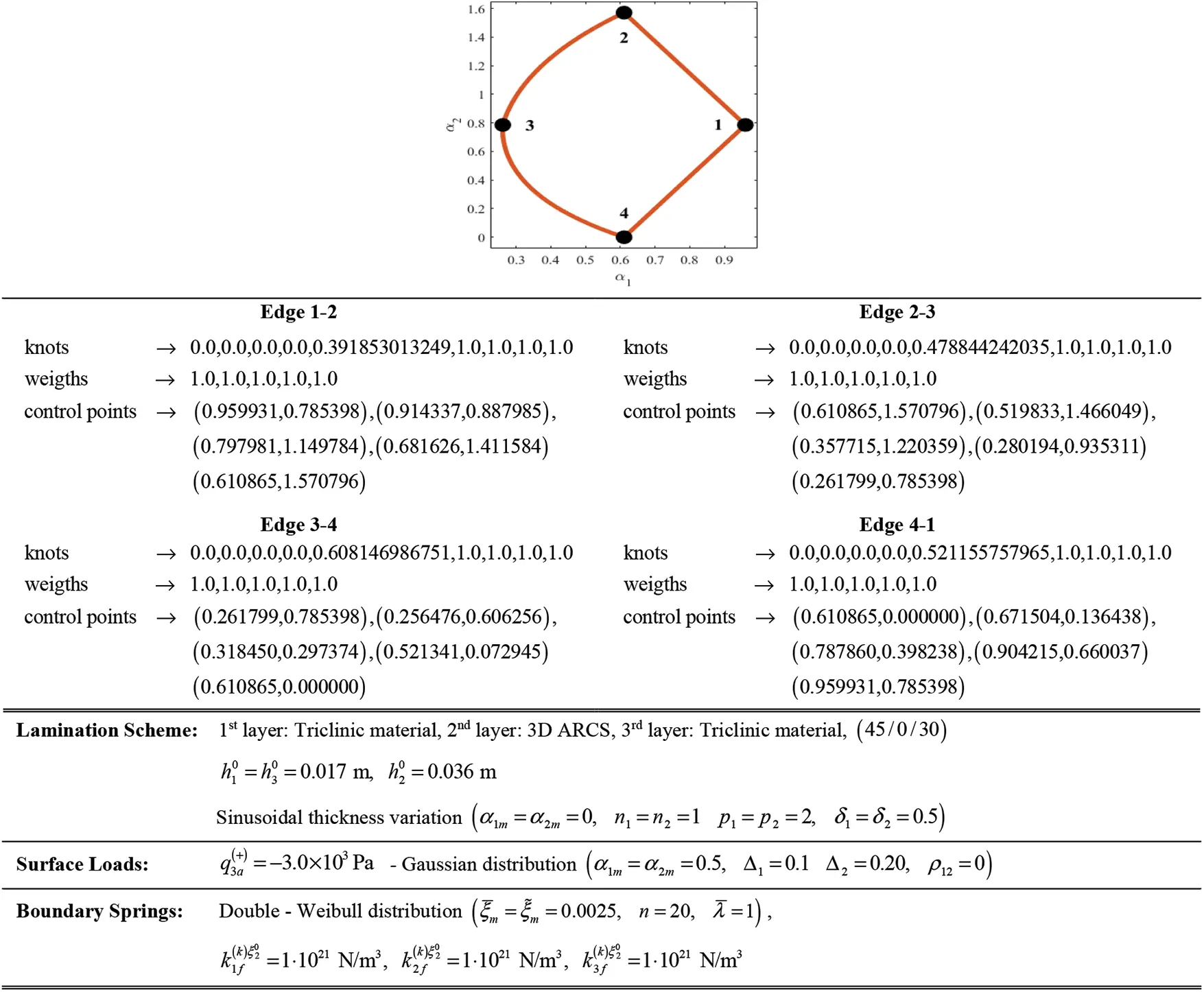
Figure 19: Geometric and mechanical properties of a super elliptic panel of revolution of mapped geometry enforced with non-conventional boundary conditions and subjected to general loads

It is interesting to note that the employed NURBS procedure allows tackling straight curves as a particular case. A general surface load has been applied to the structure, following a smooth distribution according to the Gaussian bivariate function of Eq. (67). The central core is orthotropic, in line with the 3D ARCS employed for the rectangular plate; since it has already been shown that the LD4 simulation predicts well the refined 3D FEM solutions, this time the LW model has been adopted as a reference structural response. Moreover, since the lamination scheme is characterized by a central softcore and two external layers of triclinic material (142), the ESL solution has been calculated only with the employment of the zigzag hypothesis on the displacement field and various N-th kinematic expansion orders, according to what exerted in Eq. (27). The static deflections, computed at (0.25(ξ11−ξ10),0.25(ξ21−ξ20)), have been collected in Fig. 20. The in-plane displacement field components show that the EDZ4 assumption in both the strong and weak form best fits the results provided by the LD4 reference simulation in both triclinic layers and in the central 3D ARCS softcore. A great accordance is noticed between different approaches involving the strong and weak form of the EDZ4 structural theory. The shape of the distribution coming from the LD4 model is also well predicted by the ESL theory with zigzag functions characterized by N=4. On the other hand, the ESL solution provides a linear distribution in the displacement field in-plane components, whereas the LD4 simulation accounts for a nonlinear dispersion due to the softcore behaviour of the lattice layer. Referring to the through-the-thickness dispersions of the three-dimensional strains reported in Fig. 21, the squeezing phenomenon due to the presence of the 3D ARCS is evident. The EDZ4 theory in both its strong and weak formulation well predicts the deformations of the two external triclinic layers. Referring to the central core, the structural response is strongly dependent on the choice of the axiomatic displacement field thickness function. The employment of a higher order for the kinematic expansion provides results close to the LW outcomes, especially for the case of out-of-plane distortions γ13,γ23 and stretching component ε3.

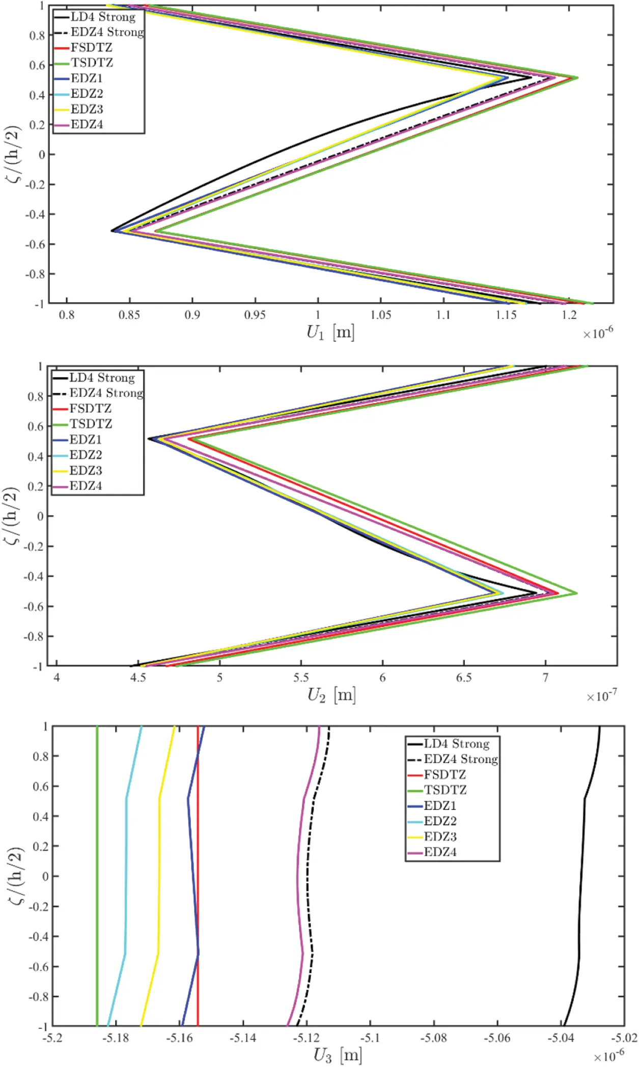
Figure 20: Through-the-thickness distributions at (0.25(ξ11−ξ10),0.25(ξ21−ξ20)) of the three-dimensional displacement field vector U(α1,α2,ζ) of a super elliptic panel of revolution of arbitrary shape composed of two generally anisotropic layers under static loads (q~3(+)=−3000Pa) enforced with general boundary conditions (BDDDKFCF)

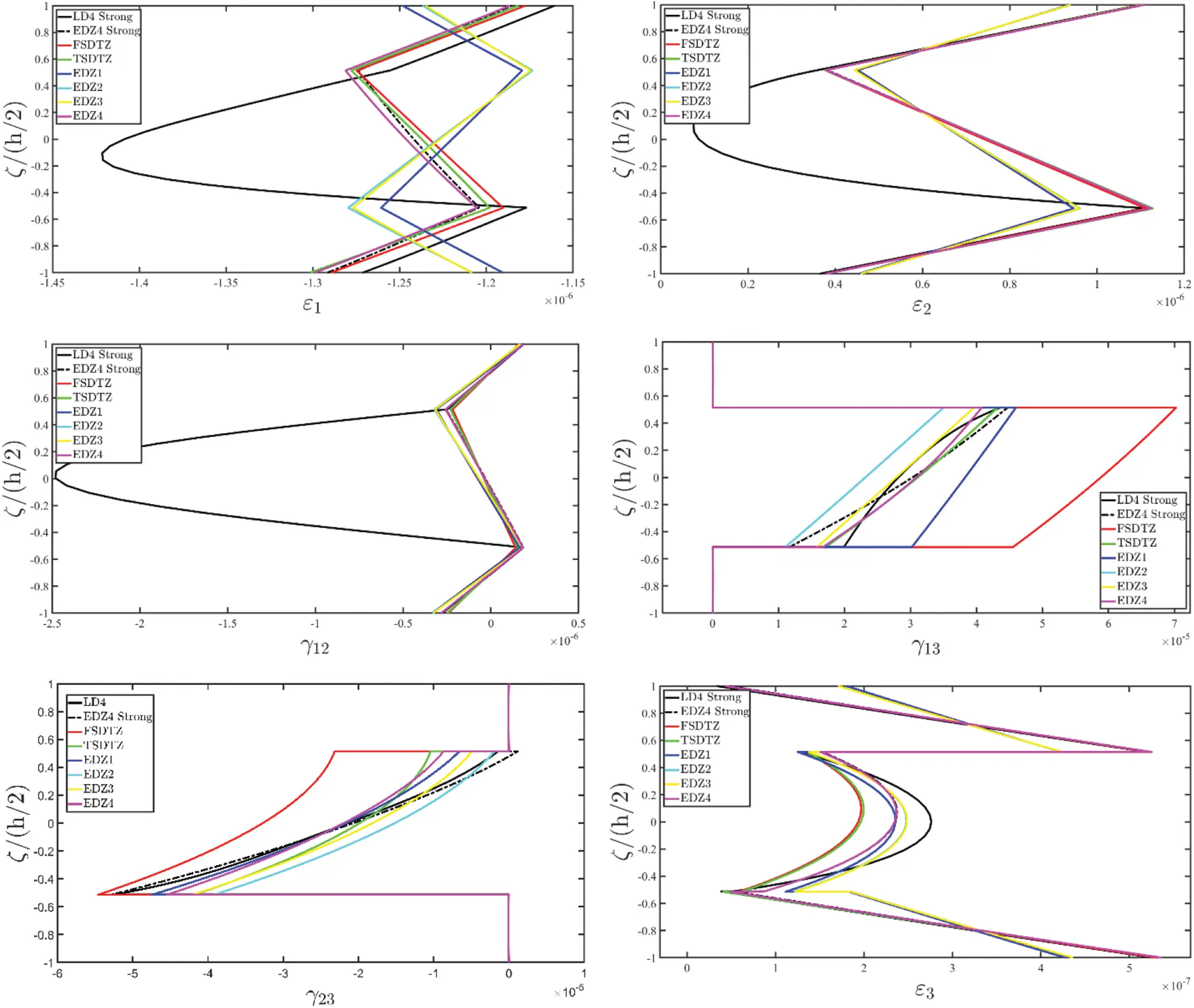
Figure 21: Through-the-thickness distributions at (0.25(ξ11−ξ10),0.25(ξ21−ξ20)) of the three-dimensional strain vector ε(α1,α2,ζ) of a super elliptic panel of revolution of arbitrary shape composed of two generally anisotropic layers under static loads (q~3(+)=−3000Pa) enforced with general boundary conditions (BDDDKFCF)

Some concluding remarks are made on the three-dimensional stress components σ(α1,α2,ζ), as visible in Fig. 22. Since the equivalent elastic stiffnesses provided via the implementation of the engineering constants from Eqs. (151) and (152) are lower than those of a triclinic material provided in Eq. (142), in the central area of the structure very low in-plane normal and shear stresses are obtained. On the contrary, the two outer layers provide higher values of stresses, following a linear dispersion. A parabolic distribution is traced in the τ13,τ23 and σ3 representation, due to the enforcement of the equilibrium boundary conditions. A great accordance can be found between the LD4 reference simulation and the results obtained from the ESL solution regardless the maximum order of the kinematic expansion.

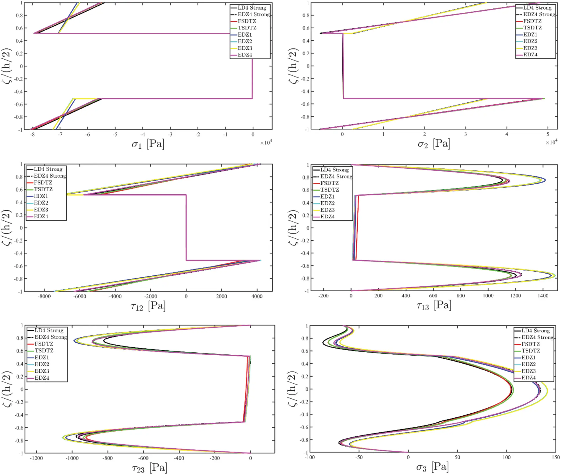
Figure 22: Through-the-thickness distributions at (0.25(ξ11−ξ10),0.25(ξ21−ξ20)) of the three-dimensional stress vector σ(α1,α2,ζ) of a super elliptic panel of revolution of arbitrary shape composed of two generally anisotropic layers under static loads (q~3(+)=−3000Pa) enforced with general boundary conditions (BDDDKFCF)

Above all, it is shown that the proposed formulation is very reliable for the static study of arbitrarily-shaped laminated structures under static loads. Moreover, the accuracy of the model is not affected by the presence of a layer with lattice features.

10  Conclusions

In the present work, an ESL formulation based on higher order theories has been proposed for the linear static analysis of structures with double curvature and arbitrary shape accounting for a general assessment of external boundary conditions and lamination schemes, involving a generalized in-plane and out-of-plane dispersion of linear elastic springs. Furthermore, a general shape of the external loads has been provided based on various bivariate distributions. The formulation has been developed following a generalized variational approach, accounting for an interpolation of the field variable of higher order based on Lagrange polynomials and a generic number of grid points. Differently from classical variational approaches, the structural problem is now characterized by refined shape functions, with a significant reduction in the computational cost. As a matter of fact, the computation of the fundamental matrices is performed by means of a numerical integration throughout the entire physical domain.

In the post-processing phase, an equilibrium-based recovery procedure has allowed for an exact fulfilment of boundary conditions coming from the externally applied surface loads. A series of validating examples has been proposed, where the static response of structures with different curvatures has been successfully checked. The accuracy of the solution has been evaluated from a direct comparison of the results obtained from refined 3D and LW theories. The proposed formulation has been demonstrated to be very reliable for disparate situations in terms of materials, lamination schemes and load conditions.

Funding Statement: The authors received no specific funding for this study.

Conflicts of Interest: The authors declare that they have no conflicts of interest to report regarding the present study.

References

 1.  Schlaich, J., Schober, H. (1996). Glass-covered grid-shells. Structural Engineering International, 6, 88–90. DOI 10.2749/101686696780495716. [Google Scholar] [CrossRef]

 2.  Adriaenssens, S., Block, P., Veenendaal, D., Williams, C. (2014). Shell structures for architecture: Form finding and optimization. New York: Routledge. [Google Scholar]

 3.  Nielsen, M. W. D., Johnson, K. J., Rhead, A. T., Butler, R. (2017). Laminate design for optimised in-plane performance and ease of manufacture. Composite Structures, 177(1), 119–128. DOI 10.1016/j.compstruct.2017.06.061. [Google Scholar] [CrossRef]

 4.  Vannucci, P., Verchery, G. (2002). A new method for generating fully isotropic laminates. Composite Structures, 58(1), 75–82. DOI 10.1016/S0263-8223(02)00038-7. [Google Scholar] [CrossRef]

 5.  Clyne, T. W., Hull, D. (2019). An introduction to composite materials. Cambridge: Cambridge University Press. [Google Scholar]

 6.  Kalamkarov, A. L., Hassan, E. M., Georgiades, A. V., Savi, M. A. (2009). Asymptotic homogenization model for 3D grid-reinforced composite structures with generally orthotropic reinforcements. Composite Structures, 89(2), 186–196. DOI 10.1016/j.compstruct.2008.07.026. [Google Scholar] [CrossRef]

 7.  Richardson, J. N., Adriaenssens, S., Coelho, R. F., Bouillard, P. (2013). Coupled form-finding and grid optimization approach for single layer grid shells. Engineering Structures, 52(1), 230–239. DOI 10.1016/j.engstruct.2013.02.017. [Google Scholar] [CrossRef]

 8.  Schek, H. J. (1974). The force density method for form finding and computation of general networks. Computer Methods in Applied Mechanics and Engineering, 3(1), 115–134. DOI 10.1016/0045-7825(74)90045-0. [Google Scholar] [CrossRef]

 9.  Qatu, M. S., Sullivan, R. W., Wang, W. (2010). Recent research advances on the dynamic analysis of composite shells: 2000–2009. Composite Structures, 93(1), 14–31. DOI 10.1016/j.compstruct.2010.05.014. [Google Scholar] [CrossRef]

10. Sokolnikoff, I. S., Specht, R. D. (1956). Mathematical theory of elasticity. New York: McGraw-Hill. [Google Scholar]

11. Dindarloo, M. H., Li, L., Dimitri, R., Tornabene, F. (2020). Nonlocal elasticity response of doubly-curved nanoshells. Symmetry, 12(3), 466. DOI 10.3390/sym12030466. [Google Scholar] [CrossRef]

12. Oden, J. T., Reddy, J. N. (2012). An introduction to the mathematical theory of finite elements. New York: Dover Publications Inc. [Google Scholar]

13. Zienkiewicz, O. C., Taylor, R. L., Nithiarasu, P., Zhu, J. Z. (1977). The finite element method. London: McGraw-Hill. [Google Scholar]

14. Akin, J. E. (2005). Finite element analysis with error estimators: An introduction to the fem and adaptive error analysis for engineering students. Burlington: Elsevier. [Google Scholar]

15. Gould, P. L. (1999). Analysis of plates and shells. Upper Saddle River: Prentice-Hall. [Google Scholar]

16. Tornabene, F., Bacciocchi, M. (2018). Anisotropic doubly-curved shells. Higher-order strong and weak formulations for arbitrarily shaped shell structures. Bologna: Esculapio. [Google Scholar]

17. Tornabene, F., Viola, E., Fantuzzi, N. (2013). General higher-order equivalent single layer theory for free vibrations of doubly-curved laminated composite shells and panels. Composite Structures, 104(1), 94–117. DOI 10.1016/j.compstruct.2013.04.009. [Google Scholar] [CrossRef]

18. Reddy, J. N., Robbins Jr, D. H. (1994). Theories and computational models for composite laminates. Applied Mechanics Reviews, 47(6), 147–169. DOI 10.1115/1.3111076. [Google Scholar] [CrossRef]

19. Tornabene, F., Viscoti, M., Dimitri, R. (2022). Generalized higher order layerwise theory for the dynamic study of anisotropic doubly-curved shells with a mapped geometry. Engineering Analysis with Boundary Elements, 134(1), 147–183. DOI 10.1016/j.enganabound.2021.09.017. [Google Scholar] [CrossRef]

20. Tornabene, F., Fantuzzi, N., Bacciocchi, M., Reddy, J. N. (2017). An equivalent layer-wise approach for the free vibration analysis of thick and thin laminated and sandwich shells. Applied Sciences, 7(1), 17. DOI 10.3390/app7010017. [Google Scholar] [CrossRef]

21. Ferreira, A. J. M. (2005). Analysis of composite plates using a layerwise theory and multiquadrics discretization. Mechanics of Advanced Materials and Structures, 12(2), 99–112. DOI 10.1080/15376490490493952. [Google Scholar] [CrossRef]

22. Kim, H. S., Chattopadhyay, A., Ghoshal, A. (2003). Dynamic analysis of composite laminates with multiple delamination using improved layerwise theory. AIAA Journal, 41(9), 1771–1779. DOI 10.2514/2.7295. [Google Scholar] [CrossRef]

23. Cho, Y. B., Averill, R. C. (2000). First-order zig-zag sublaminate plate theory and finite element model for laminated composite and sandwich panels. Composite Structures, 50(1), 1–15. DOI 10.1016/S0263-8223(99)00063-X. [Google Scholar] [CrossRef]

24. D’Ottavio, M. (2016). A sublaminate generalized unified formulation for the analysis of composite structures. Composite Structures, 142(1), 187–199. [Google Scholar]

25. Pantano, A., Averill, R. C. (2000). A 3D zig-zag sublaminate model for analysis of thermal stresses in laminated composite and sandwich plates. Journal of Sandwich Structures & Materials, 2(3), 288–312. DOI 10.1177/109963620000200307. [Google Scholar] [CrossRef]

26. Reddy, J. N. (1993). An evaluation of equivalent-single-layer and layerwise theories of composite laminates. Composite Structures, 25(1–4), 21–35. DOI 10.1016/0263-8223(93)90147-I. [Google Scholar] [CrossRef]

27. Tornabene, F., Viscoti, M., Dimitri, R., Reddy, J. N. (2021). Higher order theories for the vibration study of doubly-curved anisotropic shells with a variable thickness and isogeometric mapped geometry. Composite Structures, 267(1), 113829. DOI 10.1016/j.compstruct.2021.113829. [Google Scholar] [CrossRef]

28. MacNeal, R. H. (1998). Perspective on finite elements for shell analysis. Finite Elements in Analysis and Design, 30(3), 175–186. DOI 10.1016/S0168-874X(98)00005-5. [Google Scholar] [CrossRef]

29. Ozkul, T. A., Ture, U. (2004). The transition from thin plates to moderately thick plates by using finite element analysis and the shear locking problem. Thin-Walled Structures, 42(10), 1405–1430. DOI 10.1016/j.tws.2004.05.003. [Google Scholar] [CrossRef]

30. Cottrell, J. A., Hughes, T. J., Bazilevs, Y. (2009). Isogeometric analysis: Toward integration of CAD and FEA. Chichester: John Wiley & Sons. [Google Scholar]

31. Tornabene, F., Fantuzzi, N., Ubertini, F., Viola, E. (2015). Strong formulation finite element method based on differential quadrature: A survey. ASME Applied Mechanics Reviews, 67(2), 20801. DOI 10.1115/1.4028859. [Google Scholar] [CrossRef]

32. Nguyen, V. P., Anitescu, C., Bordas, S. P., Rabczuk, T. (2015). Isogeometric analysis: An overview and computer implementation aspects. Mathematics and Computers in Simulation, 117(1), 89–116. DOI 10.1016/j.matcom.2015.05.008. [Google Scholar] [CrossRef]

33. Hughes, T. J. R., Reali, A., Sangalli, G. (2010). Efficient quadrature for NURBS-based isogeometric analysis. Computer Methods in Applied Mechanics and Engineering, 199(5–8), 301–313. DOI 10.1016/j.cma.2008.12.004. [Google Scholar] [CrossRef]

34. Kiran, R., Nguyen-Thanh, N., Huang, J., Zhou, K. (2021). Buckling analysis of cracked orthotropic 3D plates and shells via an isogeometric-reproducing kernel particle method. Theoretical and Applied Fracture Mechanics, 114 (1), 102993. DOI 10.1016/j.tafmec.2021.102993. [Google Scholar] [CrossRef]

35. Huang, J., Nguyen-Thanh, N., Gao, J., Fan, Z., Zhou, K. (2022). Static, free vibration, and buckling analyses of laminated composite plates via an isogeometric meshfree collocation approach. Composite Structures, 285(1), 115011. DOI 10.1016/j.compstruct.2021.115011. [Google Scholar] [CrossRef]

36. Tornabene, F., Fantuzzi, N., Bacciocchi, M. (2017). A new doubly-curved shell element for the free vibrations of arbitrarily shaped laminated structures based on weak formulation isogeometric analysis. Composite Structures, 171(1), 429–461. DOI 10.1016/j.compstruct.2017.03.055. [Google Scholar] [CrossRef]

37. Tornabene, F., Viscoti, M., Dimitri, R. (2022). Equivalent single layer higher order theory based on a weak formulation for the dynamic analysis of anisotropic doubly-curved shells with arbitrary geometry and variable thickness. Thin-Walled Structures, 174(1), 109119. DOI 10.1016/j.tws.2022.109119. [Google Scholar] [CrossRef]

38. Piegl, L., Tiller, W. (1987). Curve and surface constructions using rational B-splines. Computer-Aided Design, 19(9), 485–498. DOI 10.1016/0010-4485(87)90234-X. [Google Scholar] [CrossRef]

39. Piegl, L., Tiller, W. (1996). The NURBS book. Berlin: Springer Science & Business Media. [Google Scholar]

40. Tu, L. W. (2017). Differential geometry: Connections, curvature, and characteristic classes. Medford: Springer. [Google Scholar]

41. Berger, M., Gostiaux, B. (2012). Differential geometry: Manifold. New York: Springer Science & Business Media. [Google Scholar]

42. Khare, R. K., Kant, T., Garg, A. K. (2003). Closed-form thermo-mechanical solutions of higher-order theories of cross-ply laminated shallow shells. Composite Structures, 59(3), 313–340. DOI 10.1016/S0263-8223(02)00245-3. [Google Scholar] [CrossRef]

43. Kant, T., Menon, M. P. (1989). Higher-order theories for composite and sandwich cylindrical shells with C0 finite element. Computers & Structures, 33(5), 1191–1204. DOI 10.1016/0045-7949(89)90458-6. [Google Scholar] [CrossRef]

44. Reddy, J. N., Liu, C. (1985). A Higher-order shear deformation theory of laminated elastic shells. International Journal of Engineering Science, 23(3), 319–330. DOI 10.1016/0020-7225(85)90051-5. [Google Scholar] [CrossRef]

45. Reddy, J. N. (1987). A generalization of two-dimensional theories of laminated composite plates. Communications in Applied Numerical Methods, 3(3), 173–180. DOI 10.1002/(ISSN)1555-2047. [Google Scholar] [CrossRef]

46. Washizu, K. (1975). Variational methods in elasticity and plasticity. Oxford: Pergamon Press. [Google Scholar]

47. Tornabene, F., Fantuzzi, N., Viola, E., Carrera, E. (2014). Static analysis of doubly-curved anisotropic shells and panels using CUF approach, differential geometry and differential quadrature method. Composite Structures, 107(1), 675–697. DOI 10.1016/j.compstruct.2013.08.038. [Google Scholar] [CrossRef]

48. Mantari, J. L., Soares, C. G. (2012). Bending analysis of thick exponentially graded plates using a new trigonometric higher order shear deformation theory. Composite Structures, 94(6), 1991–2000. DOI 10.1016/j.compstruct.2012.01.005. [Google Scholar] [CrossRef]

49. Carrera, E., Filippi, M., Zappino, E. (2013). Laminated beam analysis by polynomial, trigonometric, exponential and zig–zag theories. European Journal of Mechanics-A/Solids, 41(1), 58–69. DOI 10.1016/j.euromechsol.2013.02.006. [Google Scholar] [CrossRef]

50. Mantari, J. L., Soares, C. G. (2013). A novel higher-order shear deformation theory with stretching effect for functionally graded plates. Composites Part B: Engineering, 45(1), 268–281. DOI 10.1016/j.compositesb.2012.05.036. [Google Scholar] [CrossRef]

51. Benson, D. J., Bazilevs, Y., Hsu, M. C., Hughes, T. (2010). Isogeometric shell analysis: The Reissner–Mindlin shell. Computer Methods in Applied Mechanics and Engineering, 199(5–8), 276–289. DOI 10.1016/j.cma.2009.05.011. [Google Scholar] [CrossRef]

52. Liu, F. L., Liew, K. M. (1998). Static analysis of Reissner-Mindlin plates by differential quadrature element method. Journal of Applied Mechanics, 65(3), 705–710. DOI 10.1115/1.2789114. [Google Scholar] [CrossRef]

53. Reddy, J. N. (1984). A simple higher-order theory for laminated composite plates. ASME Journal of Applied Mechanics, 51(4), 745–752. DOI 10.1115/1.3167719. [Google Scholar] [CrossRef]

54. Aliaga, J. W., Reddy, J. N. (2004). Nonlinear thermoelastic analysis of functionally graded plates using the third-order shear deformation theory. International Journal of Computational Engineering Science, 5(4), 753–779. DOI 10.1142/S1465876304002666. [Google Scholar] [CrossRef]

55. Aagaah, M. R., Mahinfalah, M., Jazar, G. N. (2006). Natural frequencies of laminated composite plates using third order shear deformation theory. Composite Structures, 72(3), 273–279. DOI 10.1016/j.compstruct.2004.11.012. [Google Scholar] [CrossRef]

56. Carrera, E., Brischetto, S., Cinefra, M., Soave, M. (2011). Effects of thickness stretching in functionally graded plates and shells. Composites Part B: Engineering, 42(2), 123–133. DOI 10.1016/j.compositesb.2010.10.005. [Google Scholar] [CrossRef]

57. Whitney, J. M., Pagano, N. J. (1970). Shear deformation in heterogeneous anisotropic plates. ASME Journal of Applied Mechanics, 37(4), 1031–1036. DOI 10.1115/1.3408654. [Google Scholar] [CrossRef]

58. Tessler, A., di Sciuva, M., Gherlone, M. (2010). A consistent refinement of first-order shear deformation theory for laminated composite and sandwich plates using improved zigzag kinematics. Journal of Mechanics of Materials and Structures, 5(2), 341–367. DOI 10.2140/jomms.2010.5.341. [Google Scholar] [CrossRef]

59. Tessler, A., di Sciuva, M., Gherlone, M. (2009). A refined zigzag beam theory for composite and sandwich beams. Journal of Composite Materials, 43(9), 1051–1081. DOI 10.1177/0021998308097730. [Google Scholar] [CrossRef]

60. Iurlaro, L., Gherlone, M. D., di Sciuva, M., Tessler, A. (2013). Assessment of the refined zigzag theory for bending, vibration, and buckling of sandwich plates: A comparative study of different theories. Composite Structures, 106(1), 777–792. DOI 10.1016/j.compstruct.2013.07.019. [Google Scholar] [CrossRef]

61. Tessler, A. (2015). Refined zigzag theory for homogeneous, laminated composite, and sandwich beams derived from Reissner’s mixed variational principle. Meccanica, 50(10), 2621–2648. DOI 10.1007/s11012-015-0222-0. [Google Scholar] [CrossRef]

62. Zhu, B., Yu, T. X., Tao, X. M. (2007). An experimental study of in-plane large shear deformation of woven fabric composite. Composites Science and Technology, 67(2), 252–261. DOI 10.1016/j.compscitech.2006.08.011. [Google Scholar] [CrossRef]

63. Mohammed, U., Lekakou, C., Dong, L., Bader, M. G. (2000). Shear deformation and micromechanics of woven fabrics. Composites Part A: Applied Science and Manufacturing, 31(4), 299–308. DOI 10.1016/S1359-835X(99)00081-0. [Google Scholar] [CrossRef]

64. Carrera, E., Brischetto, S. (2009). A survey with numerical assessment of classical and refined theories for the analysis of sandwich plates. Applied Mechanics Reviews, 62(1), 10803. DOI 10.1115/1.3013824. [Google Scholar] [CrossRef]

65. Toledano, A., Murakami, H. (1987). A high-order laminated plate theory with improved in-plane responses. International Journal of Solids Structures, 23(1), 111–131. DOI 10.1016/0020-7683(87)90034-5. [Google Scholar] [CrossRef]

66. Murakami, H. (1986). Laminated composite plate theory with improved in-plane responses. ASME Journal of Applied Mechanics, 53(3), 661–666. DOI 10.1115/1.3171828. [Google Scholar] [CrossRef]

67. Reddy, J. N., Wang, C. M., Lee, K. H. (1997). Relationships between bending solutions of classical and shear deformation beam theories. International Journal of Solids and Structures, 34(26), 3373–3384. DOI 10.1016/S0020-7683(96)00211-9. [Google Scholar] [CrossRef]

68. Cheng, Z. Q., Batra, R. C. (2000). Deflection relationships between the homogeneous Kirchhoff plate theory and different functionally graded plate theories. Archives of Mechanics, 52(1), 143–158. [Google Scholar]

69. Madabhusi-Raman, P., Davalos, J. F. (1996). Static shear correction factor for laminated rectangular beams. Composites Part B: Engineering, 27(3–4), 285–293. DOI 10.1016/1359-8368(95)00014-3. [Google Scholar] [CrossRef]

70. Zghal, S., Frikha, A., Dammak, F. (2017). Static analysis of functionally graded carbon nanotube-reinforced plate and shell structures. Composite Structures, 176(1), 1107–1123. DOI 10.1016/j.compstruct.2017.06.015. [Google Scholar] [CrossRef]

71. Civalek, Ö. (2014). Geometrically nonlinear dynamic and static analysis of shallow spherical shell resting on two-parameters elastic foundations. International Journal of Pressure Vessels and Piping, 113(1), 1–9. DOI 10.1016/j.ijpvp.2005.10.005. [Google Scholar] [CrossRef]

72. Kraus, H. (1967). Thin elastic shells: An introduction to the theoretical foundations and the analysis of their static and dynamic behaviour. London: Wiley. [Google Scholar]

73. Mantari, J. L., Bonilla, E. M., Soares, C. G. (2014). A new tangential-exponential higher order shear deformation theory for advanced composite plates. Composites Part B: Engineering, 60(1), 319–328. DOI 10.1016/j.compositesb.2013.12.001. [Google Scholar] [CrossRef]

74. Tornabene, F., Viola, E. (2013). Static analysis of functionally graded doubly-curved shells and panels of revolution. Meccanica, 48(4), 901–930. DOI 10.1007/s11012-012-9643-1. [Google Scholar] [CrossRef]

75. Tornabene, F., Fantuzzi, N., Bacciocchi, M., Viola, E. (2015). A new approach for treating concentrated loads in doubly-curved composite deep shells with variable radii of curvature. Composite Structures, 131(1), 433–452. DOI 10.1016/j.compstruct.2015.05.049. [Google Scholar] [CrossRef]

76. Eftekhari, S. A. (2015). A differential quadrature procedure with regularization of the Dirac-delta function for numerical solution of moving load problem. Latin American Journal of Solids and Structures, 12(7), 1241–1265. DOI 10.1590/1679-78251417. [Google Scholar] [CrossRef]

77. Eftekhari, S. A. (2015). A note on mathematical treatment of the Dirac-delta function in the differential quadrature bending and forced vibration analysis of beams and rectangular plates subjected to concentrated loads. Applied Mathematical Modelling, 39(20), 6223–6242. DOI 10.1016/j.apm.2015.01.063. [Google Scholar] [CrossRef]

78. Eftekhari, S. A. (2016). A differential quadrature procedure with direct projection of the heaviside function for numerical solution of moving load problem. Latin American Journal of Solids and Structures, 13(9), 1763–1781. DOI 10.1590/1679-78252251. [Google Scholar] [CrossRef]

79. Zhang, Z., Zhong, Z. (2008). Bending analysis of Kirchhoff plates by wavelet-based differential quadrature method. Chinese Journal of Computational Mechanics, 25(6), 863–867. [Google Scholar]

80. Wang, X., Wang, Y., Xu, S. (2012). DSC analysis of a simply supported anisotropic rectangular plate. Composite Structures, 94(8), 2576–2584. DOI 10.1016/j.compstruct.2012.03.005. [Google Scholar] [CrossRef]

81. Zhang, L. H., Lai, S. K., Wang, C., Yang, J. (2021). DSC regularized Dirac-delta method for dynamic analysis of FG graphene platelet-reinforced porous beams on elastic foundation under a moving load. Composite Structures, 255(1), 112865. DOI 10.1016/j.compstruct.2020.112865. [Google Scholar] [CrossRef]

82. Tornabene, F., Fantuzzi, N., Bacciocchi, M. (2016). On the mechanics of laminated doubly-curved shells subjected to point and line loads. International Journal of Engineering Science, 109(1), 115–164. DOI 10.1016/j.ijengsci.2016.09.001. [Google Scholar] [CrossRef]

83. Jones, I. A. (1998). Approximate solutions to the orthotropic pinched cylinder problem. Composite Structures, 42(1), 73–91. DOI 10.1016/S0263-8223(97)00005-6. [Google Scholar] [CrossRef]

84. Jones, I. A. (2002). Pinched cylinder benchmarks for shear deformable laminated shells. Plastics, Rubber and Composites, 31(6), 249–261. DOI 10.1179/146580102225005072. [Google Scholar] [CrossRef]

85. Zhang, J. W. (1991). A parametric study of pinched orthotropic cylindrical shells. Journal of Computational and Applied Mathematics, 35(1–3), 319–330. DOI 10.1016/0377-0427(91)90219-A. [Google Scholar] [CrossRef]

86. Shu, C., Chew, Y. T., Richards, B. E. (1995). Generalized differential and integral quadrature and their application to solve boundary layer equations. International Journal for Numerical Methods in Fluids, 21(9), 723–733. DOI 10.1002/(ISSN)1097-0363. [Google Scholar] [CrossRef]

87. Loy, C. T., Lam, K. Y., Shu, C. (1997). Analysis of cylindrical shells using generalized differential quadrature. Shock and Vibration, 4(3), 193–198. DOI 10.1155/1997/538754. [Google Scholar] [CrossRef]

88. Shu, C. (2000). Differential quadrature and its application in engineering. Berlin, Heidelberg: Springer Science & Business Media. [Google Scholar]

89. Shu, C., Richards, B. E. (1992). Application of generalized differential quadrature to solve two-dimensional incompressible Navier-Stokes equations. International Journal for Numerical Methods in Fluids, 15(7), 791–798. DOI 10.1002/(ISSN)1097-0363. [Google Scholar] [CrossRef]

90. Shu, C., Chew, Y. T., Khoo, B. C., Yeo, K. S. (1996). Solutions of three-dimensional boundary layer equations by global methods of generalized differential-integral quadrature. International Journal of Numerical Methods for Heat & Fluid Flow, 6(2), 61–75. DOI 10.1108/09615539610113109. [Google Scholar] [CrossRef]

91. Shu, C., Du, H. (1997). Implementation of clamped and simply supported boundary conditions in the GDQ free vibration analysis of beams and plates. International Journal of Solids and Structures, 34(7), 819–835. DOI 10.1016/S0020-7683(96)00057-1. [Google Scholar] [CrossRef]

92. Kiani, Y., Eslami, M. R. (2016). The GDQ approach to thermally nonlinear generalized thermoelasticity of a hollow sphere. International Journal of Mechanical Sciences, 118(1), 195–204. DOI 10.1016/j.ijmecsci.2016.09.019. [Google Scholar] [CrossRef]

93. Mahmure, A., Tornabene, F., Dimitri, R., Kuruoglu, N. (2021). Free vibration of thin-walled composite shell structures reinforced with uniform and linear carbon nanotubes: Effect of the elastic foundation and nonlinearity. Nanomaterials, 11(8), 2090. DOI 10.3390/nano11082090. [Google Scholar] [CrossRef]

94. Tornabene, F., Viscoti, M., Dimitri, R., Aiello, M. A. (2021). Higher-order modeling of anisogrid composite lattice structures with complex geometries. Engineering Structures, 244(1), 112686. DOI 10.1016/j.engstruct.2021.112686. [Google Scholar] [CrossRef]

95. Shu, C., Chew, Y. T. (1998). On the equivalence of generalized differential quadrature and highest order finite difference scheme. Computer Methods in Applied Mechanics and Engineering, 155(3–4), 249–260. DOI 10.1016/S0045-7825(97)00150-3. [Google Scholar] [CrossRef]

96. Shu, C., Chen, W., Xue, H., Du, H. (2001). Numerical study of grid distribution effect on accuracy of DQ analysis of beams and plates by error estimation of derivative approximation. International Journal for Numerical Methods in Engineering, 51(2), 159–179. DOI 10.1002/nme.150. [Google Scholar] [CrossRef]

97. Shu, C., Chen, W. (1999). On optimal selection of interior points for applying discretized boundary conditions in DQ vibration analysis of beams and plates. Journal of Sound and Vibration, 222(2), 239–257. DOI 10.1006/jsvi.1998.2041. [Google Scholar] [CrossRef]

98. Fazzolari, F. A., Viscoti, M., Dimitri, R., Tornabene, F. (2021). 1D-Hierarchical Ritz and 2D-GDQ formulations for the free vibration analysis of circular/elliptical cylindrical shells and beam structures. Composite Structures, 258(1), 113338. DOI 10.1016/j.compstruct.2020.113338. [Google Scholar] [CrossRef]

99. Kamarian, S., Salim, M., Dimitri, R., Tornabene, F. (2016). Free vibration analysis of conical shells reinforced with agglomerated carbon nanotubes. International Journal of Mechanical Sciences, 108–109(1), 157–165. DOI 10.1016/j.ijmecsci.2016.02.006. [Google Scholar] [CrossRef]

100. Nejati, M., Asanjarani, A., Dimitri, R., Tornabene, F. (2017). Static and free vibration analysis of functionally graded conical shells reinforced by carbon nanotubes. International Journal of Mechanical Sciences, 130(1), 383–398. DOI 10.1016/j.ijmecsci.2017.06.024. [Google Scholar] [CrossRef]

101. Tornabene, F., Liverani, A., Caligiana, G. (2011). FGM and laminated doubly curved shells and panels of revolution with a free-form meridian: A 2-D GDQ solution for free vibrations. International Journal of Mechanical Sciences, 53(6), 446–470. DOI 10.1016/j.ijmecsci.2011.03.007. [Google Scholar] [CrossRef]

102. Tornabene, F., Ceruti, A. (2013). Mixed static and dynamic optimization of four-parameter functionally graded completely doubly curved and degenerate shells and panels using GDQ method. Mathematical Problems in Engineering, 2013(1), 867079. DOI 10.1155/2013/867079. [Google Scholar] [CrossRef]

103. Hong, C. C. (2021). Vibration frequency of thick functionally graded material cylindrical shells with fully homogeneous equation and third-order shear deformation theory under thermal environment. Journal of Vibration and Control, 27(7–8), 2004–2017. DOI 10.1177/1077546320951663. [Google Scholar] [CrossRef]

104. Tornabene, F., Viscoti, M., Dimitri, R. (2021). Higher order formulations for doubly-curved shell structures with a honeycomb core. Thin-Walled Structures, 164(1), 107789. DOI 10.1016/j.tws.2021.107789. [Google Scholar] [CrossRef]

105. Vannucci, P., Verchery, G. (2001). Stiffness design of laminates using the polar method. International Journal of Solids and Structures, 38(50–51), 9281–9294. DOI 10.1016/S0020-7683(01)00177-9. [Google Scholar] [CrossRef]

106. Catapano, A., Montemurro, M. (2014). A Multi-scale approach for the optimum design of sandwich plates with honeycomb core. Part I: Homogenisation of core properties. Composite Structures, 118(1), 664–676. DOI 10.1016/j.compstruct.2014.07.057. [Google Scholar] [CrossRef]

107. Malek, S., Gibson, L. (2015). Effective elastic properties of periodic hexagonal honeycombs. Mechanics of Materials, 91(1), 226–240. DOI 10.1016/j.mechmat.2015.07.008. [Google Scholar] [CrossRef]

108. Gibson, L. J. (1989). Modelling the mechanical behavior of cellular materials. Materials Science and Engineering: A, 110(1), 1–36. [Google Scholar]

109. Wang, X. T., Wang, B., Li, X. W., Ma, L. (2017). Mechanical properties of 3D re-entrant auxetic cellular structures. International Journal of Mechanical Sciences, 131–132(1), 396–407. DOI 10.1016/j.ijmecsci.2017.05.048. [Google Scholar] [CrossRef]

110. Wang, X. T., Li, X. W., Ma, L. (2016). Interlocking assembled 3D auxetic cellular structures. Materials & Design, 99(1), 467–476. DOI 10.1016/j.matdes.2016.03.088. [Google Scholar] [CrossRef]

111. Li, X., Lu, Z., Yang, Z., Yang, C. (2017). Directions dependence of the elastic properties of a 3D augmented re-entrant cellular structure. Materials & Design, 134(1), 151–162. DOI 10.1016/j.matdes.2017.08.024. [Google Scholar] [CrossRef]

112. Zienkiewicz, O. C., Zhu, J. Z. (1992). The superconvergent patch recovery and a posteriori error estimates. Part 1: The recovery technique. International Journal for Numerical Methods in Engineering, 33(7), 1331–1364. DOI 10.1002/(ISSN)1097-0207. [Google Scholar] [CrossRef]

113. Zienkiewicz, O. C., Zhu, J. Z. (1995). Superconvergence and the superconvergent patch recovery. Finite Elements in Analysis and Design, 19(1–2), 11–23. DOI 10.1016/0168-874X(94)00054-J. [Google Scholar] [CrossRef]

114. Mitropolsky, I. A. (1967). Averaging method in non-linear mechanics. International Journal of Non-Linear Mechanics, 2(1), 69–96. DOI 10.1016/0020-7462(67)90020-0. [Google Scholar] [CrossRef]

115. Carstensen, C., Funken, S. A. (2001). Averaging technique for FE–A posteriori error control in elasticity. Part I: Conforming FEM. Computer Methods in Applied Mechanics and Engineering, 190(18–19), 2483–2498. DOI 10.1016/S0045-7825(00)00248-6. [Google Scholar] [CrossRef]

116. Katili, I., Maknun, I. J., Tjahjono, E., Alisjahbana, I. (2017). Error estimation for the DKMQ24 shell element using various recovery methods. International Journal of Technology, 6(1), 1060–1069. [Google Scholar]

117. Tornabene, F., Reddy, J. N. (2013). FGM and laminated doubly-curved and degenerate shells resting on nonlinear elastic foundations: A GDQ solution for static analysis with a posteriori stress and strain recovery. Journal of Indian Institute of Science, 93(4), 635–688. [Google Scholar]

118. Tornabene, F., Fantuzzi, N., Bacciocchi, M. (2017). Linear static response of nanocomposite plates and shells reinforced by agglomerated carbon nanotubes. Composites Part B: Engineering, 115(1), 449–476. DOI 10.1016/j.compositesb.2016.07.011. [Google Scholar] [CrossRef]

119. Tornabene, F., Liverani, A., Caligiana, G. (2012). Static analysis of laminated composite curved shells and panels of revolution with a posteriori shear and normal stress recovery using generalized differential quadrature method. International Journal of Mechanical Sciences, 61(1), 71–87. DOI 10.1016/j.ijmecsci.2012.05.007. [Google Scholar] [CrossRef]

120. Tornabene, F., Fantuzzi, N., Viola, E., Batra, R. C. (2015). Stress and strain recovery for functionally graded free-form and doubly-curved sandwich shells using higher-order equivalent single layer theory. Composite Structures, 119(1), 67–89. DOI 10.1016/j.compstruct.2014.08.005. [Google Scholar] [CrossRef]

121. Tornabene, F., Fantuzzi, N., Bacciocchi, M. (2018). Strong and weak formulations based on differential and integral quadrature methods for the free vibration analysis of composite plates and shells: Convergence and accuracy. Engineering Analysis with Boundary Elements, 92(1), 3–37. DOI 10.1016/j.enganabound.2017.08.020. [Google Scholar] [CrossRef]

122. Tornabene, F., Fantuzzi, N., Bacciocchi, M. (2018). DiQuMASPAB: Differential quadrature for mechanics of anisotropic shells, plates, arches and beams. Bologna: Esculapio. [Google Scholar]

Appendix A. Higher order coefficients for boundary conditions

In the previous paragraphs, referring to a generic τ-th kinematic expansion order with τ=0,…,N+1, a relation has been provided in Eq. (57) in a compact matrix form that computes the generalized stress resultant vector S(τ)αi of Eq. (52) for αi=α1,α2,α3 in terms of generalized displacement field component vector u(τ) introduced in Eq. (26). In the following, we report an extended version of coefficients Ogr(τη)αiαj of the matrix O(τη)αiαj, being i,j,r=1,2,3 and g=1,…,9. Since the fundamental governing equations have been assessed in a IN×IM discrete grid, fundamental coefficients have been provided in the correspondent discrete form O~gr(τη)αiαj, defined as follows:

O~gr(τη)αiαj=O→gr(1)(τη)αiαj∘ςα1(1)α2(0)+O→gr(2)(τη)αiαj∘ςα1(0)α2(1)+O→gr(3)(τη)αiαj∘ςα1(0)α2(0)(A1)

where ςα1(n)α2(m) contains the GDQ weighting coefficients for the derivative of the (n+m)-th order referred to the principal directions of the shell α1,α2. For the sake of completeness, it should be recalled that the symbol ∘ stands for the Hadamard product. In the following, the interested reader can find the extended version of O→gr(s)(τη)αiαj, setting g=1,…,9, s=1,2,3 and i,j,r=1,2,3.

First column of the generalized operator

O→11(1)(τη)αiα1=A→1o−1∘A→11(20)(τη)[00]αiα1O→11(2)(τη)αiα1=A→2o−1∘A→16(11)(τη)[00]αiα1O→11(3)(τη)αiα1=A→1o−1∘A→2o−1∘(A→12(11)(τη)[00]αiα1∘ςα1(1)α2(0)A→2−A→16(20)(τη)[00]αiα1∘ςα1(0)α2(1)A→1)−R→1o−1∘A→14(20)(τη)[00]αiα1+A→14(10)(τη)[01]αiα1(A2)

O→21(1)(τη)αiα1=A→1o−1∘A→12(11)(τη)[00]αiα1O→21(2)(τη)α1α1=A→2o−1∘A→26(02)(τη)[00]αiα1O→21(3)(τη)α1α1=A→1o−1∘A→2o−1∘(A→22(02)(τη)[00]αiα1∘ςα1(1)α2(0)A→2−A→26(11)(τη)[00]αiα1∘ςα1(0)α2(1)A→1)−R→1o−1∘A→24(11)(τη)[00]αiα1+A→24(01)(τη)[01]αiα1(A3)

O→31(1)(τη)αiα1=A→1o−1∘A→16(20)(τη)[00]αiα1O→31(2)(τη)αiα1=A→2o−1∘A→66(11)(τη)[00]αiα1O→31(3)(τη)αiα1=A→1o−1∘A→2o−1∘(A→26(11)(τη)[00]αiα1∘ςα1(1)α2(0)A→2−A→66(20)(τη)[00]αiα1∘ςα1(0)α2(1)A→1)−R→1o−1∘A→46(20)(τη)[00]αiα1+A→46(10)(τη)[01]αiα1(A4)

O→41(1)(τη)αiα1=A→1o−1∘A→16(11)(τη)[00]αiα1O→41(2)(τη)αiα1=A→2o−1∘A→66(02)(τη)[00]αiα1O→41(3)(τη)αiα1=A→1o−1∘A→2o−1∘(A→26(02)(τη)[00]αiα1∘ςα1(1)α2(0)A→2−A→66(11)(τη)[00]αiα1∘ςα1(0)α2(1)A→1)−R→1o−1∘A→46(11)(τη)[00]αiα1+A→46(01)(τη)[01]αiα1(A5)

O→51(1)(τη)αiα1=A→1o−1∘A→14(20)(τη)[00]αiα1O→51(2)(τη)αiα1=A→2o−1∘A→46(11)(τη)[00]αiα1O→51(3)(τη)αiα1=A→1o−1∘A→2o−1∘(A→24(11)(τη)[00]αiα1∘ςα1(1)α2(0)A→2−A→46(20)(τη)[00]αiα1∘ςα1(0)α2(1)A→1)−R→1o−1∘A→44(20)(τη)[00]αiα1+A→44(10)(τη)[01]αiα1(A6)

O→61(1)(τη)αiα1=A→1o−1∘A→15(11)(τη)[00]αiα1O→61(2)(τη)αiα1=A→2o−1∘A→56(02)(τη)[00]αiα1O→61(3)(τη)αiα1=A→1o−1∘A→2o−1∘(A→25(02)(τη)[00]αiα1∘ςα1(1)α2(0)A→2−A→56(11)(τη)[00]αiα1∘ςα1(0)α2(1)A→1)−R→1o−1∘A→45(11)(τη)[00]αiα1+A→45(01)(τη)[01]αiα1(A7)

O→71(1)(τη)αiα1=A→1o−1∘A→14(10)(τη)[10]αiα1O→71(2)(τη)αiα1=A→2o−1∘A→46(01)(τη)[10]αiα1O→71(3)(τη)αiα1=A→1o−1∘A→2o−1∘(A→24(01)(τη)[10]αiα1∘ςα1(1)α2(0)A→2−A→46(10)(τη)[10]αiα1∘ςα1(0)α2(1)A→1)−R→1o−1∘A→44(10)(τη)[10]αiα1+A→44(00)(τη)[11]αiα1(A8)

O→81(1)(τη)αiα1=A→1o−1∘A→15(10)(τη)[10]αiα1O→81(2)(τη)αiα1=A→2o−1∘A→56(01)(τη)[10]αiα1O→81(3)(τη)αiα1=A→1o−1∘A→2o−1∘(A→25(01)(τη)[10]αiα1∘ςα1(1)α2(0)A→2−A→56(10)(τη)[10]αiα1∘ςα1(0)α2(1)A→1)−R→1o−1∘A→45(10)(τη)[10]αiα1+A→45(00)(τη)[11]αiα1(A9)

O→91(1)(τη)αiα1=A→1o−1∘A→13(10)(τη)[10]αiα1O→91(2)(τη)αiα1=A→2o−1∘A→36(01)(τη)[10]αiα1O→91(3)(τη)αiα1=A→1o−1∘A→2o−1∘(A→23(01)(τη)[10]αiα1∘ςα1(1)α2(0)A→2−A→36(10)(τη)[10]αiα1∘ςα1(0)α2(1)A→1)−R→1o−1∘A→34(10)(τη)[10]αiα1+A→34(00)(τη)[11]αiα1(A10)

Second column of the generalized operator

O→12(1)(τη)αiα2=A→1o−1∘A→16(20)(τη)[00]αiα2O→12(2)(τη)αiα2=A→2o−1∘A→12(11)(τη)[00]αiα2O→12(3)(τη)αiα2=A→1o−1∘A→2o−1∘(−A→16(11)(τη)[00]αiα2∘ςα1(1)α2(0)A→2+A→11(20)(τη)[00]αiα2∘ςα1(0)α2(1)A→1)−R→2o−1∘A→15(11)(τη)[00]αiα2+A→15(10)(τη)[01]αiα2(A11)

O→22(1)(τη)αiα2=A→1o−1∘A→26(11)(τη)[00]αiα2O→22(2)(τη)αiα2=A→2o−1∘A→22(02)(τη)[00]αiα2O→22(3)(τη)αiα2=A→1o−1∘A→2o−1∘(−A→26(02)(τη)[00]αiα2∘ςα1(1)α2(0)A→2+A→12(11)(τη)[00]αiα2∘ςα1(0)α2(2)A→1)−R→2o−1∘A→25(02)(τη)[00]αiα2+A→25(01)(τη)[01]αiα2(A12)

O→32(1)(τη)αiα2=A→1o−1∘A→66(20)(τη)[00]αiα2O→32(2)(τη)αiα2=A→2o−1∘A→26(11)(τη)[00]αiα2O→32(3)(τη)αiα2=A→1o−1∘A→2o−1∘(−A→66(11)(τη)[00]αiα2∘ςα1(1)α2(0)A→2+A→16(20)(τη)[00]αiα2∘ςα1(0)α2(2)A→1)−R→2o−1∘A→56(11)(τη)[00]αiα2+A→56(10)(τη)[01]αiα2(A13)

O→42(1)(τη)αiα2=A→1o−1∘A→66(11)(τη)[00]αiα2O→42(2)(τη)αiα2=A→2o−1∘A→26(02)(τη)[00]αiα2O→42(3)(τη)αiα2=A→1o−1∘A→2o−1∘(−A→66(02)(τη)[00]αiα2∘ςα1(1)α2(0)A→2+A→16(11)(τη)[00]αiα2∘ςα1(0)α2(2)A→1)−R→2o−1∘A→56(02)(τη)[00]αiα2+A→56(01)(τη)[01]αiα2(A14)

O→52(1)(τη)αiα2=A→1o−1∘A→46(20)(τη)[00]αiα2O→52(2)(τη)αiα2=A→2o−1∘A→24(11)(τη)[00]αiα2O→52(3)(τη)αiα2=A→1o−1∘A→2o−1∘(−A→46(11)(τη)[00]αiα2∘ςα1(1)α2(0)A→2+A→14(20)(τη)[00]αiα2∘ςα1(0)α2(2)A→1)−R→2o−1∘A→45(11)(τη)[00]αiα2+A→45(10)(τη)[01]αiα2(A15)

O→62(1)(τη)αiα2=A→1o−1∘A→56(11)(τη)[00]αiα2O→62(2)(τη)αiα2=A→2o−1∘A→25(02)(τη)[00]αiα2O→62(3)(τη)αiα2=A→1o−1∘A→2o−1∘(−A→56(02)(τη)[00]αiα2∘ςα1(1)α2(0)A→2+A→15(11)(τη)[00]αiα2∘ςα1(0)α2(2)A→1)−R→2o−1∘A→55(02)(τη)[00]αiα2+A→55(01)(τη)[01]αiα2(A16)

O→72(1)(τη)αiα2=A→1o−1∘A→46(10)(τη)[10]αiα2O→72(2)(τη)αiα2=A→2o−1∘A→24(01)(τη)[10]αiα2O→72(3)(τη)αiα2=A→1o−1∘A→2o−1∘(−A→46(01)(τη)[10]αiα2∘ςα1(1)α2(0)A→2+A→14(10)(τη)[10]αiα2∘ςα1(0)α2(2)A→1)−R→2o−1∘A→45(01)(τη)[10]αiα2+A→45(00)(τη)[11]αiα2(A17)

O→82(1)(τη)αiα2=A→1o−1∘A→56(10)(τη)[10]αiα2O→82(2)(τη)αiα2=A→2o−1∘A→25(01)(τη)[10]αiα2O→82(3)(τη)αiα2=A→1o−1∘A→2o−1∘(−A→56(01)(τη)[10]αiα2∘ςα1(1)α2(0)A→2+A→15(10)(τη)[10]αiα2∘ςα1(0)α2(2)A→1)−R→2o−1∘A→55(01)(τη)[10]αiα2+A→55(00)(τη)[11]αiα2(A18)

O→92(1)(τη)αiα2=A→1o−1∘A→36(10)(τη)[10]αiα2O→92(2)(τη)αiα2=A→2o−1∘A→23(01)(τη)[10]αiα2O→92(3)(τη)αiα2=A→1o−1∘A→2o−1∘(−A→36(01)(τη)[10]αiα2∘ςα1(1)α2(0)A→2+A→13(10)(τη)[10]αiα2∘ςα1(0)α2(2)A→1)−R→2o−1∘A→35(01)(τη)[10]αiα2+A→35(00)(τη)[11]αiα2(A19)

Third column of the generalized operator

O→13(1)(τη)αiα3=A→1o−1∘A→14(20)(τη)[00]αiα3O→13(2)(τη)αiα3=A→2o−1∘A→15(11)(τη)[00]αiα3O→13(3)(τη)αiα3=R→1o−1∘A→11(20)(τη)[00]αiα3+R→2o−1∘A→12(11)(τη)[00]αiα3+A→13(10)(τη)[01]αiα3(A20)

O→23(1)(τη)αiα3=A→1o−1∘A→24(11)(τη)[00]αiα3O→23(2)(τη)αiα3=A→2o−1∘A→25(02)(τη)[00]αiα3O→23(3)(τη)αiα3=R→1o−1∘A→12(11)(τη)[00]αiα3+R→2o−1∘A→22(02)(τη)[00]αiα3+A→23(01)(τη)[01]αiα3(A21)

O→33(1)(τη)αiα3=A→1o−1∘A→46(20)(τη)[00]αiα3O→33(2)(τη)αiα3=A→2o−1∘A→56(11)(τη)[00]αiα3O→33(3)(τη)αiα3=R→1o−1∘A→16(20)(τη)[00]αiα3+R→2o−1∘A→26(11)(τη)[00]αiα3+A→36(10)(τη)[01]αiα3(A22)

O→43(1)(τη)αiα3=A→1o−1∘A→46(11)(τη)[00]αiα3O→43(2)(τη)αiα3=A→2o−1∘A→56(02)(τη)[00]αiα3O→43(3)(τη)αiα3=R→1o−1∘A→16(11)(τη)[00]αiα3+R→2o−1∘A→26(02)(τη)[00]αiα3+A→36(01)(τη)[01]αiα3(A23)

O→53(1)(τη)αiα3=A→1o−1∘A→44(20)(τη)[00]αiα3O→53(2)(τη)αiα3=A→2o−1∘A→45(11)(τη)[00]αiα3O→53(3)(τη)αiα3=R→1o−1∘A→14(20)(τη)[00]αiα3+R→2o−1∘A→24(11)(τη)[00]αiα3+A→34(10)(τη)[01]αiα3(A24)

O→63(1)(τη)αiα3=A→1o−1∘A→45(11)(τη)[00]αiα3O→63(2)(τη)αiα3=A→2o−1∘A→55(02)(τη)[00]αiα3O→63(3)(τη)αiα3=R→1o−1∘A→15(11)(τη)[00]αiα3+R→2o−1∘A→25(02)(τη)[00]αiα3+A→35(01)(τη)[01]αiα3(A25)

O→73(1)(τη)αiα3=A→1o−1∘A→44(10)(τη)[10]αiα3O→73(2)(τη)αiα3=A→2o−1∘A→45(01)(τη)[10]αiα3O→73(3)(τη)αiα3=R→1o−1∘A→14(10)(τη)[10]αiα3+R→2o−1∘A→24(01)(τη)[10]αiα3+A→34(00)(τη)[11]αiα3(A26)

O→83(1)(τη)αiα3=A→1o−1∘A→45(10)(τη)[10]αiα3O→83(2)(τη)αiα3=A→2o−1∘A→55(01)(τη)[10]αiα3O→83(3)(τη)αiα3=R→1o−1∘A→15(10)(τη)[10]αiα3+R→2o−1∘A→25(01)(τη)[10]αiα3+A→35(00)(τη)[11]αiα3(A27)

O→93(1)(τη)αiα3=A→1o−1∘A→34(10)(τη)[10]αiα3O→93(2)(τη)αiα3=A→2o−1∘A→35(01)(τη)[10]αiα3O→93(3)(τη)αiα3=R→1o−1∘A→13(10)(τη)[10]αiα3+R→2o−1∘A→23(01)(τη)[10]αiα3+A→33(00)(τη)[11]αiα3(A28)

Appendix B. Higher order fundamental stiffness matrix coefficients

In the present section we report the complete expression of the fundamental coefficients KΦ(τη)αjαi of the stiffness matrix of Eq. (62), defined for each τ,η=0,…,N+1 and αi,αj=α1,α2,α3 principal direction of the shell. As can be seen, a formulation employing the Kronecker tensorial product ⊗ is provided, as well as vectors lα1,lα2 of the Lagrange interpolating polynomials of Eq. (34), as well as their first order derivatives lα1(1),lα2(1). For the sake of completeness, the terms of the generalized stiffness matrix A(τη)αiαj are computed according to the expression reported in Eq. (54) for each τ,η=0,…,N+1 and αi,αj=α1,α2,α3. All the terms at issue are collected by row.

First row of the fundamental stiffness matrix

KΦ(τη)α 1α 1=(Bα 1)TA(τη)α 1α 1Bα 1=A 11(20)(τη)[ 00 ]α1α1A 12((lα2)Tlα2)⊗((lα1(1))Tlα1(1))+A 16(11)(τη)[ 00 ]α1α1A 1A 2(((lα2)Tlα2(1))⊗((lα1(1))Tlα1)+((lα2(1))Tlα2)⊗((lα1)Tlα1(1)))+A 66(02)(τη)[ 00 ]α1α1A 22((lα2(1))Tlα2(1))⊗((lα1)Tlα1)+(A 12(11)(τη)[ 00 ]α1α1A 12A 2∂A 2∂α1−A 16(20)(τη)[ 00 ]α1α1A 12A 2∂A 1∂α2−A14(20)(τη)[ 00 ]α1α1A 1R 1)(((lα2)Tlα2)⊗((lα1(1))Tlα1)+((lα2)Tlα2)⊗((lα1)Tlα1(1)))+A14(10)(τη)[ 01 ]α1α1A 1((lα2)Tlα2)⊗((lα1(1))Tlα1)+A14(10)(τη)[ 10 ]α1α1A 1((lα2)Tlα2)⊗((lα1)Tlα1(1))+(A 26(02)(τη)[ 00 ]α1α1A 1A 22∂A 2∂α1−A 66(11)(τη)[ 00 ]α1α1A 1A 22∂A 1∂α2−A46(11)(τη)[ 00 ]α1α1A 2R 1)(((lα2)Tlα2(1))⊗((lα1)Tlα1)+((lα2(1))Tlα2)⊗((lα1)Tlα1))+A46(01)(τη)[ 01 ]α1α1A 2((lα2(1))Tlα2)⊗((lα1)Tlα1)+A46(01)(τη)[ 10 ]α1α1A 2((lα2)Tlα2(1))⊗((lα1)Tlα1)+( (A24(01)(τη)[ 01 ]α1α1+A24(01)(τη)[ 10 ]α1α1A 1A 2−2A24(11)(τη)[ 00 ]α1α1A 1A 2R 1)∂A 2∂α1+(−A46(10)(τη)[ 01 ]α1α1+A46(10)(τη)[ 10 ]α1α1A 1A 2+2A46(20)(τη)[ 00 ]α1α1A 1A 2R 1)∂A 1∂α2+A 22(02)(τη)[ 00 ]α1α1A 12A 22(∂A 2∂α1)2 +A 66(20)(τη)[ 00 ]α1α1A 12A 22(∂A 1∂α2)2−2A 26(11)(τη)[ 00 ]α1α1A 12A 22∂A 1∂α2∂A 2∂α1+A 44(20)(τη)[ 00 ]α1α1R 12−A 44(10)(τη)[ 01 ]α1α1+A 44(10)(τη)[ 10 ]α1α1R 1+A 44(00)(τη)[ 11 ]α1α1 )((lα2)Tlα2)⊗((lα1)Tlα1)(A29)

KΦ(τη)α 1α 2=(Bα 1)TA(τη)α 1α 2Bα 2=A 16(20)(τη)[ 00 ]α1α2A 12((lα2)Tlα2)⊗((lα1(1))Tlα1(1))+A 12(11)(τη)[ 00 ]α1α2A 1A 2((lα2)Tlα2(1))⊗((lα1(1))Tlα1)+A 66(11)(τη)[ 00 ]α1α2A 1A 2((lα2(1))Tlα2)⊗((lα1)Tlα1(1))+A 26(02)(τη)[ 00 ]α1α2A 22((lα2(1))Tlα2(1))⊗((lα1)Tlα1)+(A 11(20)(τη)[ 00 ]α1α2A 12A 2∂A 1∂α2−A 16(11)(τη)[ 00 ]α1α2A 12A 2∂A 2∂α1−A15(11)(τη)[ 00 ]α1α2A 1R 2+A15(10)(τη)[ 01 ]α1α2A 1)((lα2)Tlα2)⊗((lα1(1))Tlα1)+(A 26(11)(τη)[ 00 ]α1α2A 12A 2∂A 2∂α1−A 66(20)(τη)[ 00 ]α1α2A 12A 2∂A 1∂α2−A46(20)(τη)[ 00 ]α1α2A 1R 1+A46(10)(τη)[ 10 ]αiα2A 1)((lα2)Tlα2)⊗((lα1)Tlα1(1))+(A 22(02)(τη)[ 00 ]α1α2A 1A 22∂A 2∂α1−A 26(11)(τη)[ 00 ]α1α2A 1A 22∂A 1∂α2−A24(11)(τη)[ 00 ]α1α2A 2R 1+A24(01)(τη)[ 10 ]α1α2A 2)((lα2)Tlα2(1))⊗((lα1)Tlα1)+(A 16(11)(τη)[ 00 ]α1α2A 1A 22∂A 1∂α2−A 66(02)(τη)[ 00 ]α1α2A 1A 22∂A 2∂α1−A56(02)(τη)[ 00 ]α1α2A 2R 2+A56(01)(τη)[ 01 ]α1α2A 2)((lα2(1))Tlα2)⊗((lα1)Tlα1)+( (A46(11)(τη)[ 00 ]α1α2A 1A 2R 1−A25(02)(τη)[ 00 ]α1α2A 1A 2R 2+A25(01)(τη)[ 01 ]α1α2−A46(01)(τη)[ 10 ]α1α2A 1A 2)∂A 2∂α1+(−A14(20)(τη)[ 00 ]α1α2A 1A 2R 1+A56(11)(τη)[ 00 ]α1α2A 1A 2R 2+A14(10)(τη)[ 10 ]α1α2−A56(10)(τη)[ 01 ]α1α2A 1A 2)∂A 1∂α2+A 12(11)(τη)[ 00 ]α1α2+A 66(11)(τη)[ 00 ]α1α2A 12A 22∂A 1∂α2∂A 2∂α1−A 26(02)(τη)[ 00 ]α1α2A 12A 22(∂A 2∂α1)2−A 16(20)(τη)[ 00 ]α1α2A 12A 22(∂A 1∂α2)2 +A 45(11)(τη)[ 00 ]α1α2R 1R 2−A 45(10)(τη)[ 01 ]α1α2R 1−A 45(10)(τη)[ 10 ]α1α2R 2+A 45(00)(τη)[ 11 ]α1α2 )((lα2)Tlα2)⊗((lα1)Tlα1)(A30)

KΦ(τη)α 1α 3​ =(Bα 1)TA(τη)α 1α 3Bα 3=A14(20)(τη)[ 00 ]α1α3A 12((lα2)Tlα2)⊗((lα1(1))Tlα1(1))+A15(11)(τη)[ 00 ]α1α3A 1A 2((lα2)Tlα2(1))⊗((lα1(1))Tlα1)+A46(11)(τη)[ 00 ]α1α3A 1A 2((lα2(1))Tlα2)⊗((lα1)Tlα1(1))+A56(02)(τη)[ 00 ]α1α3A 22((lα2(1))Tlα2(1))⊗((lα1)Tlα1)+(A11(20)(τη)[ 00 ]α1α3A 1R 1+A12(11)(τη)[ 00 ]α1α3A 1R 2+A13(10)(τη)[ 01 ]α1α3A 1)((lα2)Tlα2)⊗((lα1(1))Tlα1)+(A24(11)(τη)[ 00 ]α1α3A 12A 2∂A 2∂α1−A46(20)(τη)[ 00 ]α1α3A 12A 2∂A 1∂α2+A44(10)(τη)[ 10 ]α1α3A 1−A44(20)(τη)[ 00 ]α1α3A 1R 1)((lα2)Tlα2)⊗((lα1)Tlα1(1))+(A25(02)(τη)[ 00 ]α1α3A 1A 22∂A 2∂α1−A56(11)(τη)[ 00 ]α1α3A 1A 22∂A 1∂α2+A45(01)(τη)[ 10 ]α1α3A 2−A45(11)(τη)[ 00 ]α1α3A 2R 1)((lα2)Tlα2(1))⊗((lα1)Tlα1)+(A16(11)(τη)[ 00 ]α1α3A 2R 1+A26(02)(τη)[ 00 ]α1α3A 2R 2+A36(01)(τη)[ 01 ]α1α3A 2)((lα2(1))Tlα2)⊗((lα1)Tlα1)+( (A12(11)(τη)[ 00 ]α1α3A 1A 2R 1+A22(02)(τη)[ 00 ]α1α3A 1A 2R 2+A23(01)(τη)[ 01 ]α1α3A 1A 2)∂A 2∂α1−(A16(20)(τη)[ 00 ]α1α3A 1A 2R 1+A26(11)(τη)[ 00 ]α1α3A 1A 2R 2+A36(10)(τη)[ 01 ]α1α3A 1A 2)∂A 1∂α2 −A14(20)(τη)[ 00 ]α1α3R 12−A24(11)(τη)[ 00 ]α1α3R 1R 2+A14(10)(τη)[ 10 ]α1α3−A34(10)(τη)[ 01 ]α1α3R 1+A24(01)(τη)[ 10 ]α1α3R 2+A34(00)(τη)[ 11 ]α1α3 )((lα2)Tlα2)⊗((lα1)Tlα1)(A31)

Second row of the fundamental stiffness matrix

KΦ(τη)α 2α 1=(Bα 2)TA(τη)α 2α 1Bα 1=A 16(20)(τη)[ 00 ]α2α1A 12((lα2)Tlα2)⊗((lα1(1))Tlα1(1))+A 26(02)(τη)[ 00 ]α2α1A 22((lα2(1))Tlα2(1))⊗((lα1)Tlα1)+A 66(11)(τη)[ 00 ]α2α1A 1A 2((lα2)Tlα2(1))⊗((lα1(1))Tlα1)+A 12(11)(τη)[ 00 ]α2α1A 1A 2((lα2(1))Tlα2)⊗((lα1)Tlα1(1))+(A 26(11)(τη)[ 00 ]α2α1A 12A 2∂A 2∂α1−A 66(20)(τη)[ 00 ]α2α1A 12A 2∂A 1∂α2−A46(20)(τη)[ 00 ]α2α1A 1R 1+A46(10)(τη)[ 01 ]α2α1A 1)((lα2)Tlα2)⊗((lα1(1))Tlα1)+(A 11(20)(τη)[ 00 ]α2α1A 12A 2∂A 1∂α2−A 16(11)(τη)[ 00 ]α2α1A 12A 2∂A 2∂α1−A15(11)(τη)[ 00 ]α2α1A 1R 2+A15(10)(τη)[ 10 ]α2α1A 1)((lα2)Tlα2)⊗((lα1)Tlα1(1))+(A 16(11)(τη)[ 00 ]α2α1A 1A 22∂A 1∂α2−A 66(02)(τη)[ 00 ]α2α1A 1A 22∂A 2∂α1−A56(02)(τη)[ 00 ]α2α1A 2R 2+A56(01)(τη)[ 10 ]α2α1A 2)((lα2)Tlα2(1))⊗((lα1)Tlα1)+(A 22(02)(τη)[ 00 ]α2α1A 1A 22∂A 2∂α1−A 26(11)(τη)[ 00 ]α2α1A 1A 22∂A 1∂α2−A24(11)(τη)[ 00 ]α2α1A 2R 1+A24(01)(τη)[ 01 ]α2α1A 2)((lα2(1))Tlα2)⊗((lα1)Tlα1)+( (−A14(20)(τη)[ 00 ]α2α1A 1A 2R 1+A56(11)(τη)[ 00 ]α2α1A 1A 2R 2+A14(10)(τη)[ 01 ]α2α1−A56(10)(τη)[ 01 ]α2α1A 1A 2)∂A 1∂α2+(A46(11)(τη)[ 00 ]α2α1A 1A 2R 1−A25(02)(τη)[ 00 ]α2α1A 1A 2R 2+A25(01)(τη)[ 10 ]α2α1−A46(01)(τη)[ 01 ]α2α1A 1A 2)∂A 2∂α1+A 12(11)(τη)[ 00 ]α2α1+A 66(11)(τη)[ 00 ]α2α1A 12A 22∂A 1∂α2∂A 2∂α1−A 26(02)(τη)[ 00 ]α2α1A 12A 22(∂A 2∂α1)2−A 16(20)(τη)[ 00 ]α2α1A 12A 22(∂A 1∂α2)2 +A 45(11)(τη)[ 00 ]α2α1R 2R 1−A 45(01)(τη)[ 01 ]α2α1R 2−A 45(10)(τη)[ 10 ]α2α1R 1+A 45(00)(τη)[ 11 ]α2α1 )((lα2)Tlα2)⊗((lα1)Tlα1)(A32)

KΦ(τη)α 2α 2=(Bα 2)TA(τη)α 2α 2Bα 2=A 66(20)(τη)[ 00 ]α2α2A 12((lα2)Tlα2)⊗((lα1(1))Tlα1(1))+A 26(11)(τη)[ 00 ]α2α2A 1A 2(((lα2)Tlα2(1))⊗((lα1(1))Tlα1)+((lα2(1))Tlα2)⊗((lα1)Tlα1(1)))+A 22(02)(τη)[ 00 ]α2α2A 22((lα2(1))Tlα2(1))⊗((lα1)Tlα1)+(A 16(20)(τη)[ 00 ]α2α2A 12A 2∂A 1∂α2−A 66(11)(τη)[ 00 ]α2α2A 12A 2∂A 2∂α1−A56(11)(τη)[ 00 ]α2α2A 1R 2)( ((lα2)Tlα2)⊗((lα1(1))Tlα1) +((lα2)Tlα2)⊗((lα1)Tlα1(1)) )+A56(10)(τη)[ 01 ]α2α2A 1((lα2)Tlα2)⊗((lα1(1))Tlα1)+A56(10)(τη)[ 10 ]α2α2A 1((lα2)Tlα2)⊗((lα1)Tlα1(1))+(A 12(11)(τη)[ 00 ]α2α2A 1A 22∂A 1∂α2−A 26(02)(τη)[ 00 ]α2α2A 1A 22∂A 2∂α1−A25(02)(τη)[ 00 ]α2α2A 2R 2)( ((lα2)Tlα2(1))⊗((lα1)Tlα1) +((lα2(1))Tlα2)⊗((lα1)Tlα1) )+A25(01)(τη)[ 01 ]α2α2A 2((lα2(1))Tlα2)⊗((lα1)Tlα1)+A25(01)(τη)[ 10 ]α2α2A 2((lα2)Tlα2(1))⊗((lα1)Tlα1)+( (2A56(02)(τη)[ 00 ]α2α1A 1A 2R 2−A56(01)(τη)[ 01 ]α2α1+A56(01)(τη)[ 10 ]α2α2A 1A 2)∂A 2∂α1+(−2A15(11)(τη)[ 00 ]α2α1A 1A 2R 2+A15(10)(τη)[ 01 ]α2α1+A15(10)(τη)[ 10 ]α2α2A 1A 2)∂A 1∂α2+A 66(02)(τη)[ 00 ]α2α2A 12A 22(∂A 2∂α1)2+A 11(20)(τη)[ 00 ]α2α2A 12A 22(∂A 1∂α2)2−2A 16(11)(τη)[ 00 ]α2α2A 12A 22∂A 1∂α2∂A 2∂α1+A 55(02)(τη)[ 00 ]α2α2R 22 −A 55(01)(τη)[ 01 ]α2α2+A 55(01)(τη)[ 10 ]α2α2R 2+A 55(00)(τη)[ 11 ]α2α2 )((lα2)Tlα2)⊗((lα1)Tlα1)(A33)

KΦ(τη)α 2α 3=(Bα 2)TA(τη)α 2α 3Bα 3=A46(20)(τη)[ 00 ]α2α3A 12((lα2)Tlα2)⊗((lα1(1))Tlα1(1))+A56(11)(τη)[ 00 ]α2α3A 1A 2((lα2)Tlα2(1))⊗((lα1(1))Tlα1)+A24(11)(τη)[ 00 ]α2α3A 1A 2((lα2(1))Tlα2)⊗((lα1)Tlα1(1))+A25(02)(τη)[ 00 ]α2α3A 22((lα2(1))Tlα2(1))⊗((lα1)Tlα1)+(A16(20)(τη)[ 00 ]α2α3A 1R 1+A26(11)(τη)[ 00 ]α2α3A 1R 2+A36(10)(τη)[ 01 ]α2α3A 1)((lα2)Tlα2)⊗((lα1(1))Tlα1)+(A14(20)(τη)[ 00 ]α2α3A 12A 2∂A 1∂α2−A46(11)(τη)[ 00 ]α2α3A 12A 2∂A 2∂α1+A45(10)(τη)[ 10 ]α2α3A 1−A45(11)(τη)[ 00 ]α2α3A 1R 2)((lα2)Tlα2)⊗((lα1)Tlα1(1))+(A15(11)(τη)[ 00 ]α2α3A 1A 22∂A 1∂α2−A56(02)(τη)[ 00 ]α2α3A 1A 22∂A 2∂α1+A55(01)(τη)[ 10 ]α2α3A 2−A55(02)(τη)[ 00 ]α2α3A 2R 2)((lα2)Tlα2(1))⊗((lα1)Tlα1)+(A12(11)(τη)[ 00 ]α2α3A 2R 1+A22(02)(τη)[ 00 ]α2α3A 2R 2+A23(01)(τη)[ 01 ]α2α3A 2)((lα2(1))Tlα2)⊗((lα1)Tlα1)+( (A11(20)(τη)[ 00 ]α2α3A 1A 2R 1+A12(11)(τη)[ 00 ]α2α3A 1A 2R 2+A13(10)(τη)[ 01 ]α2α3A 1A 2)∂A 1∂α2−(A16(11)(τη)[ 00 ]α2α3A 1A 2R 1+A26(02)(τη)[ 00 ]α2α3A 1A 2R 2+A36(01)(τη)[ 01 ]α2α3A 1A 2)∂A 2∂α1 −A15(11)(τη)[ 00 ]α2α3R 1R 2−A25(02)(τη)[ 00 ]α2α3R 22+A15(10)(τη)[ 10 ]α2α3R 1+A25(01)(τη)[ 10 ]α2α3−A35(01)(τη)[ 01 ]α2α3R 2+A35(00)(τη)[ 11 ]α2α3 )((lα2)Tlα2)⊗((lα1)Tlα1)(A34)

Third row of the fundamental stiffness matrix

KΦ(τη)α 3α 1=(Bα 3)TA(τη)α 3α 1Bα 1=A14(20)(τη)[ 00 ]α3α1A 12((lα2)Tlα2)⊗((lα1(1))Tlα1(1))+A46(11)(τη)[ 00 ]α3α1A 1A 2((lα2)Tlα2(1))⊗((lα1(1))Tlα1)+A15(11)(τη)[ 00 ]α3α1A 1A 2((lα2(1))Tlα2)⊗((lα1)Tlα1(1))+A56(02)(τη)[ 00 ]α3α1A 22((lα2(1))Tlα2(1))⊗((lα1)Tlα1)+(A24(11)(τη)[ 00 ]α3α1A 12A 2∂A 2∂α1−A46(20)(τη)[ 00 ]α3α1A 12A 2∂A 1∂α2−A 44(20)(τη)[ 00 ]α3α1A 1R 1+A 44(10)(τη)[ 01 ]α3α1A 1)((lα2)Tlα2)⊗((lα1(1))Tlα1)+(A 11(20)(τη)[ 00 ]α3α1A 1R 1+A 12(11)(τη)[ 00 ]α3α1A 1R 2+A 13(10)(τη)[ 10 ]α3α1A 1)((lα2)Tlα2)⊗((lα1)Tlα1(1))+(A 16(11)(τη)[ 00 ]α3α1A 2R 1+A 26(02)(τη)[ 00 ]α3α1A 2R 2+A 36(01)(τη)[ 10 ]α3α1A 2)((lα2)Tlα2(1))⊗((lα1)Tlα1)+(A25(02)(τη)[ 00 ]α3α1A 1A 22∂A 2∂α1−A56(11)(τη)[ 00 ]α3α1A 1A 22∂A 1∂α2−A 45(11)(τη)[ 00 ]α3α1A 2R 1+A 45(01)(τη)[ 01 ]α3α1A 2)((lα2(1))Tlα2)⊗((lα1)Tlα1)+( (A 12(11)(τη)[ 00 ]α3α1A 1A 2R 1+A 22(02)(τη)[ 00 ]α3α1A 1A 2R 2+A 23(01)(τη)[ 10 ]α3α1A 1A 2)∂A 2∂α1−(A 16(20)(τη)[ 00 ]α3α1A 1A 2R 1+A 26(11)(τη)[ 00 ]α3α1A 1A 2R 2+A 36(10)(τη)[ 10 ]α3α1A 1A 2)∂A 1∂α2 −A14(20)(τη)[ 00 ]α3α1R 12−A24(11)(τη)[ 00 ]α3α1R 1R 2+A14(10)(τη)[ 01 ]α3α1−A34(10)(τη)[ 10 ]α3α1R 1+A24(01)(τη)[ 01 ]α3α1R 2+A34(00)(τη)[ 11 ]α3α1 )((lα2)Tlα2)⊗((lα1)Tlα1)(A35)

KΦ(τη)α 3α 2=(Bα 3)TA(τη)α 3α 2Bα 2=A46(20)(τη)[ 00 ]α3α2A 12((lα2)Tlα2)⊗((lα1(1))Tlα1(1))+A 24(11)(τη)[ 00 ]α3α1A 1A 2((lα2)Tlα2(1))⊗((lα1(1))Tlα1)+A 56(11)(τη)[ 00 ]α3α1A 1A 2((lα2(1))Tlα2)⊗((lα1)Tlα1(1))+A 25(02)(τη)[ 00 ]α3α1A 22((lα2(1))Tlα2(1))⊗((lα1)Tlα1)+(A14(20)(τη)[ 00 ]α3α2A 12A 2∂A 1∂α2−A46(11)(τη)[ 00 ]α3α2A 12A 2∂A 2∂α1−A 45(11)(τη)[ 00 ]α3α2A 1R 2+A 45(10)(τη)[ 01 ]α3α2A 1)((lα2)Tlα2)⊗((lα1(1))Tlα1)+(A 16(20)(τη)[ 00 ]α3α2A 1R 1+A 26(11)(τη)[ 00 ]α3α2A 1R 2+A 36(10)(τη)[ 10 ]α3α2A 1)((lα2)Tlα2)⊗((lα1)Tlα1(1))+(A 12(11)(τη)[ 00 ]α3α2A 2R 1+A 22(02)(τη)[ 00 ]α3α2A 2R 2+A 23(01)(τη)[ 10 ]α3α2A 2)((lα2)Tlα2(1))⊗((lα1)Tlα1)+(A15(11)(τη)[ 00 ]α3α2A 1A 22∂A 1∂α2−A56(02)(τη)[ 00 ]α3α2A 1A 22∂A 2∂α1−A 55(02)(τη)[ 00 ]α3α2A 2R 2+A 55(01)(τη)[ 01 ]α3α2A 2)((lα2(1))Tlα2)⊗((lα1)Tlα1)+( (A 11(20)(τη)[ 00 ]α3α2A 1A 2R 1+A 12(11)(τη)[ 00 ]α3α2A 1A 2R 2+A 13(10)(τη)[ 10 ]α3α2A 1A 2)∂A 1∂α2−(A 16(11)(τη)[ 00 ]α3α2A 1A 2R 1+A 26(02)(τη)[ 00 ]α3α2A 1A 2R 2+A 36(01)(τη)[ 10 ]α3α2A 1A 2)∂A 2∂α1 −A25(02)(τη)[ 00 ]α3α2R 22−A15(11)(τη)[ 00 ]α3α2R 1R 2+A15(10)(τη)[ 01 ]α3α2R 1+A25(01)(τη)[ 01 ]α3α2−A35(01)(τη)[ 10 ]α3α2R 2+A35(00)(τη)[ 11 ]α3α2 )((lα2)Tlα2)⊗((lα1)Tlα1)(A36)

KΦ(τη)α3α3=(Bα3)TA(τη)α3α3Bα3=A44(20)(τη)[00]α3α3A12((lα2)Tlα2)⊗((lα1(1))Tlα1(1))+A45(11)(τη)[00]α3α3A1A2(((lα2)Tlα2(1))⊗((lα1(1))Tlα1)+((lα2(1))Tlα2)⊗((lα1)Tlα1(1)))+A55(02)(τη)[00]α3α3A22((lα2(1))Tlα2(1))⊗((lα1)Tlα1)+(A14(20)(τη)[00]α3α3A1R1+A24(11)(τη)[00]α3α3A1R2+A34(10)(τη)[10]α3α3A1)((lα2)Tlα2)⊗((lα1)Tlα1(1))+(A15(11)(τη)[00]α3α3A2R1+A25(02)(τη)[00]α3α3A2R2+A35(01)(τη)[10]α3α3A2)((lα2)Tlα2(1))⊗((lα1)Tlα1)+(A14(20)(τη)[00]α3α3A1R1+A24(11)(τη)[00]α3α3A1R2+A34(10)(τη)[01]α3α3A1+A15(11)(τη)[00]α3α3A2R1+A25(02)(τη)[00]α3α3A2R2+A35(01)(τη)[01]α3α3A2+A11(20)(τη)[00]α3α3R12+A22(02)(τη)[00]α3α3R22+2A12(11)(τη)[00]α3α3R1R2+A13(10)(τη)[01]α3α3+A13(10)(τη)[10]α3α3R1+A23(01)(τη)[01]α3α3+A23(01)(τη)[10]α3α3R2+A33(00)(τη)[11]α3α3)((lα2)Tlα2)⊗((lα1)Tlα1)(A37)

Appendix C. Constitutive relationship for an orthotropic medium

With particular references of numerical investigations accounting for orthotropic materials, the expressions of Cij(k) with i,j=1,…,6 and k=1,…,l of the three-dimensional constitutive relationship reported in Eq. (49) should be considered. Actually, the mechanical properties of the k-th lamina are provided in terms of the well-known engineering constants, namely the elastic moduli E1(k),E2(k),E3(k), the shear moduli G12(k),G13(k),G23(k) and the Poisson’s coefficients ν12(k),ν13(k),ν23(k) [16]:

C11(k)=1Δ(k)1−ν23(k)ν32(k)E2(k)E3(k),C22(k)=1Δ(k)1−ν13(k)ν31(k)E1(k)E3(k)C12(k)=1Δ(k)ν21(k)+ν23(k)ν31(k)E2(k)E3(k)=1Δ(k)ν12(k)+ν32(k)ν13(k)E1(k)E3(k)C13(k)=1Δ(k)ν31(k)+ν21(k)ν32(k)E2(k)E3(k)=1Δ(k)ν13(k)+ν12(k)ν23(k)E1(k)E2(k)C23(k)=1Δ(k)ν32(k)+ν12(k)ν31(k)E1(k)E3(k)=1Δ(k)ν23(k)+ν21(k)ν13(k)E1(k)E3(k)C33(k)=1Δ(k)1−ν12(k)ν21(k)E1(k)E2(k)C44(k)=G13(k),C55(k)=G23(k),C66(k)=G12(k)C16(k)=C26(k)=C14(k)=C24(k)=C64(k)=C15(k)=C25(k)=C65(k)=C45(k)=C63(k)=C43(k)=C53(k)=0(A38)

In the previous equation, quantity Δ(k) reads as follows:

Δ(k)=1−ν12(k)ν21(k)−ν23(k)ν32(k)−ν13(k)ν31(k)−2ν21(k)ν13(k)ν32(k)E1(k)E2(k)E3(k)(A39)

It should be recalled that the Poisson’s coefficients satisfy the well-known reciprocity relation [16]:

νij(k)Ei(k)=νji(k)Ej(k)fori,j=1,2,3(A40)

This work is licensed under a Creative Commons Attribution 4.0 International License, which permits unrestricted use, distribution, and reproduction in any medium, provided the original work is properly cited.