Computer Modeling in Engineering & Sciences

---

DOI: 10.32604/cmes.2022.021081

ARTICLE

Frenet Curve Couples in Three Dimensional Lie Groups

Osman Zeki Okuyucu*

Department of Mathematics, Faculty of Science and Arts, Bilecik Şeyh Edebali University, Bilecik, Turkey
*Corresponding Author: Osman Zeki Okuyucu. Email: osman.okuyucu@bilecik.edu.tr
Received: 26 December 2021; Accepted: 28 March 2022

1  Introduction

The theory of curves has an important role in differential geometry studies. In the theory of curves, one of the interesting problems is to investigate the relations between two curves. The Frenet elements of the curves have an effective role in the solution of the problem.

For example, if the principal normal vectors coincide at the corresponding points of the curves α and β, the curve couple {α,β} is called the Bertrand curve couple in a three-dimensional Euclidean space [1,2]. Similarly, if tangent vectors coincide, the curve couple {α,β} is called the involute-evolute curve couple. Also, if the normal vector of the curve α coincides with the bi-normal vector of the curve β, the curve couple {α,β} is called the Mannheim curve couple [3].

In a three-dimensional Lie group G with a bi-invariant metric, Çiftçi has defined general helices [4]. Also Okuyucu et al. have obtained slant helices and Bertrand curves in G [5,6]. Gök et al. have investigated Mannheim curves in G [7]. Recently, Yampolsky et al. have examined helices in three dimensional Lie group G, with left-invariant metric [8]. Also, many applications of curves theory are studied and still have been investigated in three dimensional Lie groups (see [9–12], etc.).

Karakuş et al. have examined the possibility of whether any Frenet plane of a given space curve in a three-dimensional Euclidean space is also any Frenet plane of another space curve in the same space [13].

In this study, we examine the possible relations between the Frenet planes of given two curves in three dimensional Lie groups with left invariant metrics.

2  Preliminaries

Let G be a three dimensional Lie group with left-invariant metric ⟨,⟩ and let g denote the Lie algebra of G which consists of the all smooth vector fields of G invariant under left translation. There are two classes of three dimensional Lie groups:

1.    If the group is unimodular, we have a (positively oriented) orthonormal frame of left-invariant vector fields {e1,e2,e3}, such that the brackets satisfy

[e1,e2]=λ3e3,[e1,e3]=λ2e2,[e2,e3]=λ1e1,

where λi are called structure constants. The constants

μi=12(λ1+λ2+λ3)−λi,

are called connection coefficients.

2.   If the group is nonunimodular, we have an othonormal frame {e1,e2,e3}, such that

[e1,e2]=αe2+βe3,[e1,e3]=−βe2+δe3,[e2,e3]=0,

see [14].

Using the Koszul formula the covariant derivatives ∇eiej can be found as in the following tables:

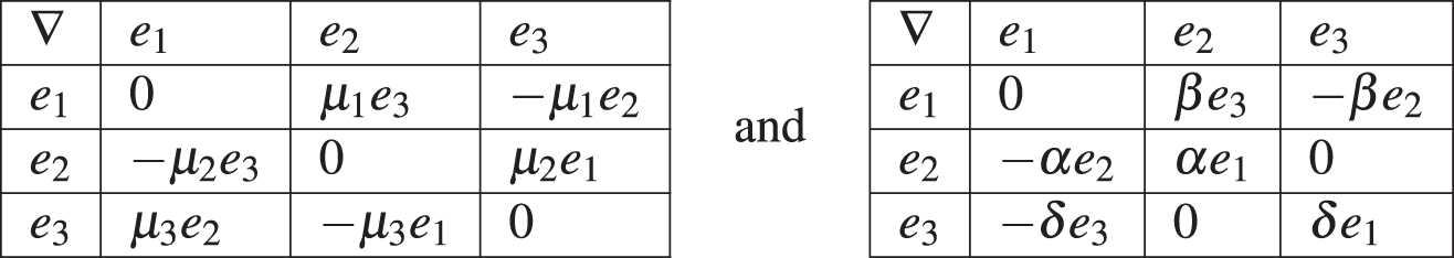
for unimodular and nonunimodular cases, respectively.

The cross-products of the vectors e1,e2,e3 are defined by the following equalities:

e1×e2=e3,e2×e3=e1,e3×e1=e2,

in three dimensional case. For unimodular and nonunimodular groups, we have ∇eiek=μ(ei)×ek, and so

∇Xek=μ(X)×ek,

for any vector field X, where μ is a affine transformation as follows:

μ(X)={μ1X1e1+μ2X2e2+μ3X3e3,βX1e1+δX3e2−αX2e3,

for unimodular and nonunimodular cases, respectively (see [8]).

We have ∇eiek=μ(ei)×ek for both groups, and so

∇Xek=μ(X)×ek,(1)

for any vector field X.

Let γ be an arc-lengthed curve on the group and T=γ˙ be the unit tangent vector field. For any vector field ξ∘γ, using the Eq. (1), we get

∇Tξ=ξ˙kek+μ(T)×ξ,(2)

where the vector field ξ˙=dξidsei is dot-derivative of the vector field ξ along the curve γ. If ξ is the restriction of a left-invariant vector field to the curve γ the ξ˙=0 (see [8]).

Let T, N and B be the vectors of the standard Frenet frame of the curve γ. We get the following equations with the help of Eq. (2):

∇TT=T˙+μ(T)×T,∇TB=B˙+μ(T)×B,∇TN=N˙+μ(T)×N.(3)

Along the curve γ, we can define a new frame {τ,v,β}, which is called dot-Frenet Frame, by

τ=T,v=1k0τ˙,β=τ×v,

where k0=|T˙|. By definition ϰ0=|β˙|.

Proposition 2.1. The dot-Frenet frame {τ,v,β} satisfies dot-Frenet formulas, namely

τ˙=kov,v˙=−k0τ+ϰ0β,β˙=−ϰ0v.

The Frenet and the dot-Frenet frames are connected by

τ=T,v=cos⁡αN+sin⁡αB,β=−sin⁡αN+cos⁡αB,

where α=α(s) is the angle function (see [8]).

Proposition 2.2. The transformation μ(T) can be given by

μ(T)=(ϰ+α˙−ϰ0)T+k0sinαN+(k−k0cosα)B,(4)

with respect to the Frenet frame {T,N,B}.

Define a group-curvature kG and a group-torsion ϰG of a curve by

kG=|μ(T)×T|,ϰG=|μ(T)×B|,

respectively. As a consequence of (4), the dot-curvature and the dot-torsion of a curve can be expressed in terms of the group-curvature kG, group-torsion ϰG of a curve, and angle function α by

kG2=(k−k0)2+4kk0sin2(α/2),ϰG2=k02sinα2+(ϰ−ϰ0+α˙)2

(see [8]).

3  Frenet Curve Couples in Three Dimensional Lie Groups

Let ζ:I⊆R→G and η:I¯⊆R→G be curves with arc-length parameter s and s¯, respectively, in three dimensional Lie group G with left-invariant metric. We denote Frenet apparatus of the curves ζ and η with {T,N,B,k0,ϰ0,α} and {T¯,N¯,B¯,k¯0,ϰ¯0,α¯}, respectively. We know that Sp{T,N}, Sp{N,B} and Sp{T,B} are the osculating plane, the normal plane and the rectifying plane of the curve ζ, respectively. And similarly, Sp{T¯,N¯}, Sp{N¯,B¯} and Sp{T¯,B¯} are the osculating plane, the normal plane and the rectifying plane of the curve η, respectively. Now we investigate the possible cases and the relations between the Frenet planes of any given two curves in three dimensional Lie groups with left invariant metrics in a step by step manner:

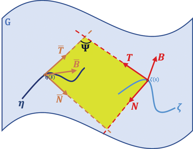
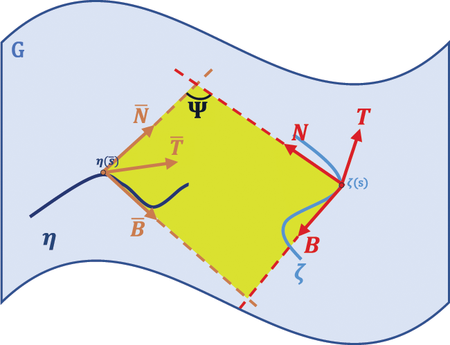
Case 1: We assume that, osculating plane of the curve ζ is the osculating plane of the curve η, that is Sp{T,N}=Sp{T¯,N¯}. As in Fig. 1, this relationship exists at the corresponding points of along the curves ζ and η.

Figure 1: Osculating planes of the curves ζ and η

So we have following relation between the curves ζ and η:

η(s¯)=ζ(s)+aT(s)+bN(s),a≠0,b≠0,(5)

where a and b are real valued non-zero functions of s.

Calculating the dot-derivative of the Eq. (5) with the help of Eqs. (3) and (4), we get

T¯(s¯)=(1+a˙−bk0cosα)1rT(s)+(ak0cosα+b˙)1rN(s)+(ak0sinα+b(−α˙+ϰ0))1rB(s),(6)

where r=ds¯ds.

We know that B is parallel to B¯, since B⊥=Sp{T,N}=Sp{T¯,N¯}=B¯⊥. If we multiply the Eq. (6) with B, we get

(ak0sinα+b(−α˙+ϰ0))1r=0orak0sinα+b(−α˙+ϰ0)=0.

And so, we have

T¯(s¯)=(1+a˙−bk0cosα)1rT(s)+(ak0cosα+b˙)1rN(s).(7)

By using Eq. (7), we can set

T¯(s¯)=cos⁡ψ(s)T(s)+sin⁡ψ(s)N(s),N¯(s¯)=−sin⁡ψ(s)T(s)+cos⁡ψ(s)N(s),(8)

where ψ is smooth angle function between T and T¯ on I and

cos⁡ψ(s)=(1+a˙−bk0cosα)1r,(9)

sin⁡ψ(s)=(ak0cosα+b˙)1r.(10)

By using the Eqs. (9) and (10), we obtain

r=(1+a˙−bk0cosα)2+(ak0cosα+b˙),2

and

bk0cos⁡α−a˙+cot⁡ψ(ak0cos⁡α+b˙)=1.

Calculating the dot-derivative of the Eq. (8) with the help of Eqs. (3) and (4), we get

r(k¯0cos⁡α¯N¯+k¯0sin⁡α¯B¯)=(−ψ˙sin⁡ψ−sin⁡ψk0cos⁡α)T+(cos⁡ψk0cos⁡α+ψ˙cos⁡ψ)N+(cos⁡ψk0sin⁡α+sin⁡ψ(−α˙+ϰ0))B.(11)

If we multiply the Eq. (11), with N¯ and B¯, respectively, we get

rk¯0cos⁡α¯=ψ˙+k0cos⁡α,(12)

rk¯0sin⁡α¯=cos⁡ψk0sin⁡α+sin⁡ψ(−α˙+ϰ0).(13)

By using Eqs. (12) and (13), we obtain

ψ˙+k0cos⁡α−cot⁡α¯(cos⁡ψk0sin⁡α+sin⁡ψ(−α˙+ϰ0))=0.

Thus we introduce the following theorem:

Theorem 3.1. Let ζ:I⊆R→G and η:I¯⊆R→G be two arc-length parametrized curves with the Frenet apparatus {T,N,B,k0,ϰ0,α} and {T¯,N¯,B¯,k¯0,ϰ¯0,α¯}, respectively, in three dimensional Lie group G with left-invariant metric. The osculating planes of these curves coincide if and only if there exist real valued non-zero functions a and b on I, such that

ak0sinα+b(−α˙+ϰ0)=0,(i)(1+a˙−bk0cosα)2+(ak0cosα+b˙)2≠0,(ii)bk0cos⁡α−a˙+cot⁡ψ(ak0cos⁡α+b˙)=1,(iii)ψ˙+k0cos⁡α−cot⁡α¯(cos⁡ψk0sin⁡α+sin⁡ψ(−α˙+ϰ0))=0.(iv)

where ψ is the angle between T and T¯ at the corresponding points of ζ and η.

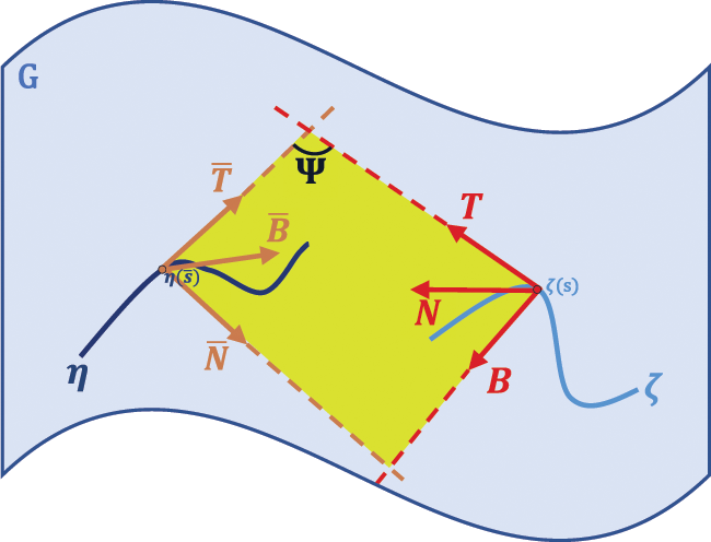
Case 2: We assume that, osculating plane of the curve ζ is the normal plane of the curve η, that is Sp{T,N}=Sp{N¯,B¯}. As in Fig. 2, this relationship exists at the corresponding points of along the curves ζ and η.

Thus, we have following relation between the curves ζ and η:

η(s¯)=ζ(s)+aT(s)+bN(s),a≠0,b≠0,(14)

where a and b are real valued non-zero functions of s.

Calculating the dot-derivative of the Eq. (14) with the help of Eqs. (3) and (4), we get

T¯(s¯)=(1+a˙−bk0cosα)1rT(s)+(ak0cosα+b˙)1rN(s)+(ak0sinα+b(−α˙+ϰ0))1rB(s),(15)

where r=ds¯ds.

Figure 2: Osculating plane of the curve ζ and normal plane of the curve η

We know that B is parallel to T¯, since B⊥=Sp{T,N}=Sp{N¯,B¯}=T¯⊥. If we multiply the Eq. (15) with T, N and B, respectively, we get

1+a˙−bk0cosα=0,ak0cosα+b˙=0,ak0sinα+b(−α˙+ϰ0)=r.

And so, we have the equation T¯(s¯)=B(s). If we calculate the dot-derivative of this equation with the help of Eqs. (3) and (4), we get

r(k¯0cosα¯N¯+k¯0sinα¯B¯)=(α˙−ϰ0)N−k0sinαT.(16)

If we multiply the Eq. (16) with N¯ and B¯, respectively, we get

rk¯0cosα¯=sin⁡ψ(α˙−ϰ0)−cosψk0sinα,(17)

rk¯0sinα¯=cos⁡ψ(α˙−ϰ0)+sinψk0sinα,(18)

where ψ is the smooth angle function between T and N¯. By using the Eqs. (17) and (18), we obtain

cotα¯=sin⁡ψ(α˙−ϰ0)−cosψk0sinαcos⁡ψ(α˙−ϰ0)+sinψk0sinα

that is

sin⁡ψ(α˙−ϰ0)−cosψk0sinα−cotα¯(cos⁡ψ(α˙−ϰ0)+sinψk0sinα)=0.

Thus we introduce the following theorem:

Theorem 3.2. Let ζ:I⊆R→G and η:I¯⊆R→G be two arc-length parametrized curves with the Frenet apparatus {T,N,B,k0,ϰ0,α} and {T¯,N¯,B¯,k¯0,ϰ¯0,α¯}, respectively, in three dimensional Lie group G with left-invariant metric. The osculating plane of the curve ζ and the normal plane of the curve η coincide if and only if there exist real valued non-zero functions a and b on I, such that:

1+a˙−bk0cos⁡α=0,(i)ak0cos⁡α+b˙=0,(ii)ak0sin⁡α+b(−α˙+ϰ0)≠0,(iii)sin⁡ψ(α˙−ϰ0)−cos⁡ψk0sin⁡α−cot⁡α¯(cos⁡ψ(α˙−ϰ0)+sin⁡ψk0sin⁡α)=0,(iv)

where ψ is the angle between T and N¯ at the corresponding points of ζ and η.

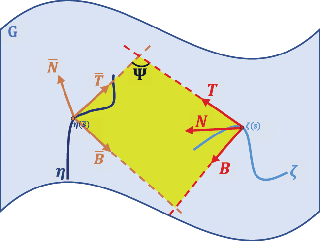
Case 3: We assume that, osculating plane of the curve ζ is the rectifying plane of the curve η, that is Sp{T,N}=Sp{T¯,B¯}. As in Fig. 3, this relationship exists at the corresponding points of along the curves ζ and η.

Figure 3: Osculating plane of the curve ζ and rectifying plane of the curve η

Thus, we have following relation between the curves ζ and η:

η(s¯)=ζ(s)+aT(s)+bN(s),a≠0,b≠0,(19)

where a and b are real valued non-zero functions of s.

Calculating the dot-derivative of the Eq. (19) with the help of Eqs. (3) and (4), we get

T¯(s¯)=(1+a˙−bk0cosα)1rT(s)+(ak0cosα+b˙)1rN(s)+(ak0sinα+b(−α˙+ϰ0))1rB(s),(20)

where r=ds¯ds.

We know that B is parallel to N¯, since B⊥=Sp{T,N}=Sp{T¯,B¯}=N¯⊥. If we multiply the Eq. (20) with B, we get

(ak0sinα+b(−α˙+ϰ0))1r=0orak0sinα+b(−α˙+ϰ0)=0.

And so, we have

T¯(s¯)=(1+a˙−bk0cosα)1rT(s)+(ak0cosα+b˙)1rN(s).(21)

By Eq. (21), we can set

T¯(s¯)=cos⁡ψ(s)T(s)+sin⁡ψ(s)N(s),B¯(s¯)=−sin⁡ψ(s)T(s)+cos⁡ψ(s)N(s),(22)

where ψ is smooth angle function between T and T¯ on I and

cos⁡ψ(s)=(1+a˙−bk0cosα)1r,(23)

sin⁡ψ(s)=(ak0cosα+b˙)1r.(24)

By using the Eqs. (23) and (24), we obtain

r=(1+a˙−bk0cosα)2+(ak0cosα+b˙)2

and

bk0cos⁡α−a˙+cot⁡ψ(ak0cos⁡α+b˙)=1.

Calculating the dot-derivative of the Eq. (22) with the help of Eqs. (3) and (4), we get

r(k¯0cos⁡α¯N¯+k¯0sin⁡α¯B¯)=(−ψ˙sin⁡ψ−sin⁡ψk0cos⁡α)T+(cos⁡ψk0cos⁡α+ψ˙cos⁡α)N+(cos⁡ψk0sin⁡α+sin⁡ψ(−α¯+ϰ0))B.(25)

If we multiply the Eq. (25), with N¯ and B¯, respectively, we get

rk¯0cos⁡α¯=cos⁡ψk0sin⁡α+sin⁡ψ(−α˙+ϰ0),(26)

rk¯0sin⁡α¯=ψ˙+k0cos⁡α.(27)

By using Eqs. (26) and (27), we obtain

cos⁡ψk0sin⁡α+sin⁡ψ(−α˙+ϰ0)−cot⁡α¯(ψ˙+k0cos⁡α)=0.

Thus we introduce the following theorem:

Theorem 3.3. Let ζ:I⊆R→G and η:I¯⊆R→G be two arc-length parametrized curves with the Frenet apparatus {T,N,B,k0,ϰ0,α} and {T¯,N¯,B¯,k¯0,ϰ¯0,α¯}, respectively, in three dimensional Lie group G with left-invariant metric. The osculating plane of the curve ζ and the rectifying plane of the curve η coincide if and only if there exist real valued non-zero functions a and b on I, such that

ak0sinα+b(−α˙+ϰ0)=0,(i)(1+a˙−bk0cosα)2+(ak0cosα+b˙)2≠0,(ii)bk0cos⁡α−a˙+cot⁡ψ(ak0cos⁡α+b˙)=1,(iii)cos⁡ψk0sin⁡α+sin⁡ψ(−α˙+ϰ0)−cot⁡α¯(ψ˙+k0cos⁡α)=0,(iv)

where ψ is the angle between T and T¯ at the corresponding points of ζ and η.

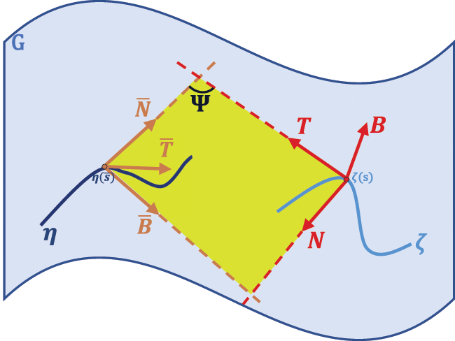
Case 4: We assume that, normal plane of the curve ζ is the osculating plane of the curve η, that is Sp{N,B}=Sp{T¯,N¯}. As in Fig. 4, this relationship exists at the corresponding points of along the curves ζ and η.

Figure 4: Normal plane of the curve ζ and osculating plane of the curve η

So we have following relation between the curves ζ and η:

η(s¯)=ζ(s)+aN(s)+bB(s),a≠0,b≠0,(28)

where a and b are real valued non-zero functions of s.

Calculating the dot-derivative of the Eq. (28) with the help of Eqs. (3) and (4), we get

T¯(s¯)=(1−ak0cosα−bk0sin⁡α)1rT(s)+(a˙+b(α˙−ϰ0))1rN(s)+(a(−α˙+ϰ0)+b˙)1rB(s),(29)

where r=ds¯ds.

We know that T is parallel to B¯, since T⊥=Sp{N,B}=Sp{T¯,N¯}=B¯⊥. If we multiply the Eq. (29) with T, we get

(1−ak0cosα−bk0sin⁡α)1r=0orak0cosα+bk0sin⁡α=1.

And so, we have

T¯(s¯)=(a˙+b(α˙−ϰ0))1rN(s)+(a(−α˙+ϰ0)+b˙)1rB(s).(30)

By the Eq. (30), we can set

T¯(s¯)=cos⁡ψ(s)N(s)+sin⁡ψ(s)B(s),N¯(s¯)=−sin⁡ψ(s)N(s)+cos⁡ψ(s)B(s),(31)

where ψ is smooth angle function between T¯ and N on I and

cos⁡ψ(s)=(a˙+b(α˙−ϰ0))1r,(32)

sin⁡ψ(s)=(a(−α˙+ϰ0)+b˙)1r.(33)

By using Eqs. (32) and (33), we obtain

r=(a˙+b(α˙−ϰ0))2+(a(−α˙+ϰ0)+b˙)2

and

a˙+b(α˙−ϰ0)+cot⁡ψ(a(−α˙+ϰ0)+b˙)=0.

Calculating the dot-derivative of the Eq. (31) with the help of Eqs. (3) and (4), we get

r(k¯0cos⁡α¯N¯+k¯0sin⁡α¯B¯)=(−cos⁡ψk0cos⁡α−sin⁡ψk0sin⁡α)T+(−ψ˙sin⁡ψ+sin⁡ψ(α˙−ϰ0))N+(cos⁡ψ(−α˙+ϰ0)+ψ˙cos⁡ψ)B.(34)

If we multiply the Eq. (34), with N¯ and B¯, respectively, we get

rk¯0cos⁡α¯=ψ˙+(−α˙+ϰ0),(35)

rk¯0sin⁡α¯=−cos⁡ψk0cos⁡α−sin⁡ψk0sin⁡α.(36)

By using Eqs. (35) and (36), we obtain

ψ˙+(−α˙+ϰ0)+cot⁡α¯k0cos⁡(ψ−α)=0.

Thus we introduce the following theorem:

Theorem 3.4. Let ζ:I⊆R→G and η:I¯⊆R→G be two arc-length parametrized curves with the Frenet apparatus {T,N,B,k0,ϰ0,α} and {T¯,N¯,B¯,k¯0,ϰ¯0,α¯}, respectively, in three dimensional Lie group G with left-invariant metric. The normal plane of the curve ζ and the osculating plane of the curve η coincide if and only if there exist real valued non-zero functions a and b on I, such that

ak0cosα+bk0sin⁡α=1,(i)(a˙+b(α˙−ϰ0))2+(a(−α˙+ϰ0)+b˙)2≠0,(ii)a˙+b(α˙−ϰ0)+cot⁡ψ(a(−α˙+ϰ0)+b˙)=0,(iii)ψ˙+(−α˙+ϰ0)+cot⁡α¯k0cos⁡(ψ−α)=0,(iv)

where ψ is the angle between T¯ and N at the corresponding points of ζ and η.

Case 5: We assume that, normal plane of the curve ζ is the normal plane of the curve η, that is Sp{N,B}=Sp{N¯,B¯}. As in Fig. 5, this relationship exists at the corresponding points of along the curves ζ and η.

Figure 5: Normal planes of the curves ζ and η

Thus, we have following relation between the curves ζ and η:

η(s¯)=ζ(s)+aN(s)+bB(s),a≠0,b≠0,(37)

where a and b are real valued non-zero functions of s.

Calculating the dot-derivative of the Eq. (37) with the help of Eqs. (3) and (4), we get

T¯(s¯)=(1−ak0cosα−bk0sin⁡α)1rT(s)+(a˙+b(α˙−ϰ0))1rN(s)+(a(−α˙+ϰ0)+b˙)1rB(s),(38)

where r=ds¯ds.

We know that T is parallel to T¯, since T⊥=Sp{N,B}=Sp{N¯,B¯}=T¯⊥. If we multiply the Eq. (38) with T, N and B, respectively, we get

ak0cos⁡α+bk0sin⁡α=1−r,a˙+b(α˙−ϰ0)=0,a(−α˙+ϰ0)+b˙=0.

And so, we have the equation T¯=T. If we calculate the dot-derivative of this equation with the help of Eqs. (3) and (4), we get

r(k¯0cos⁡α¯N¯+k¯0sin⁡α¯B¯)=k0cos⁡αN+k0sin⁡αB.(39)

If we multiply the Eq. (39) with N¯ and B¯, respectively, we get

rk¯0cos⁡α¯=cos⁡ψk0cos⁡α+sin⁡ψk0sin⁡α,(40)

rk¯0sin⁡α¯=−sin⁡ψk0cos⁡α+cos⁡ψk0sin⁡α,(41)

where ψ is the smooth angle function between N and N¯. By using the Eqs. (40) and (41), we obtain

cot⁡α¯=cos⁡ψk0cos⁡α+sin⁡ψk0sin⁡α−sin⁡ψk0cos⁡α+cos⁡ψk0sin⁡α

that is

cot⁡α¯=cos⁡(ψ−α)sin⁡(α−ψ).

This means that,

α−ψ=α¯+kπ,k∈Z.

Thus we introduce the following theorem:

Theorem 3.5. Let ζ:I⊆R→G and η:I¯⊆R→G be two arc-length parametrized curves with the Frenet apparatus {T,N,B,k0,ϰ0,α} and {T¯,N¯,B¯,k¯0,ϰ¯0,α¯}, respectively, in three dimensional Lie group G with left-invariant metric. The normal planes of these curves coincide if and only if there exist real valued non-zero functions a and b on I, such that:

1−ak0cosα−bk0sin⁡α≠0,(i)a˙+b(α˙−ϰ0)=0,(ii)a(−α˙+ϰ0)+b˙=0,(iii)α−ψ=α¯+kπ,k∈Z,(iv)

where ψ is the angle between N and N¯ at the corresponding points of ζ and η.

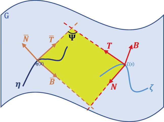
Case 6: We assume that, normal plane of the curve ζ is the rectifying plane of the curve η, that is Sp{N,B}=Sp{T¯,B¯}. As in Fig. 6, this relationship exists at the corresponding points of along the curves ζ and η.

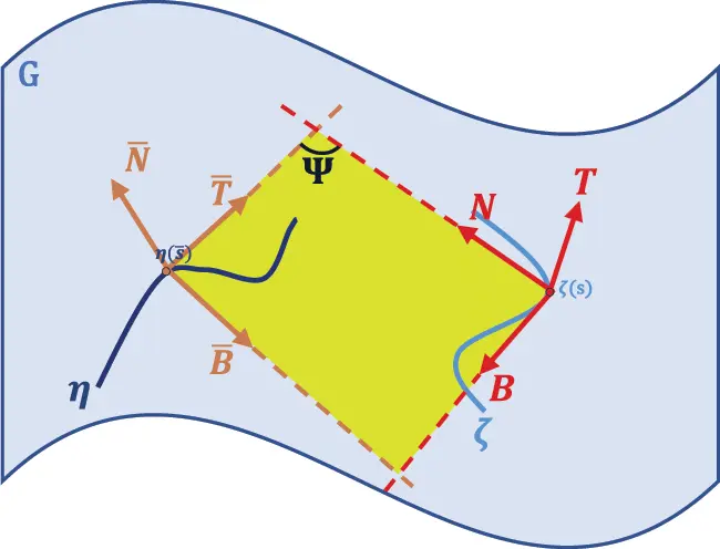
Figure 6: Normal plane of the curve ζ and rectifying plane of the curve η

Thus, we have following relations between the curves ζ and η:

η(s¯)=ζ(s)+aN(s)+bB(s),a≠0,b≠0,(42)

where a and b are real valued non-zero functions of s.

Calculating the dot-derivative of the Eq. (42) with the help of Eqs. (3) and (4), we get

T¯(s¯)=(1−ak0cosα−bk0sin⁡α)1rT(s)+(a˙+b(α˙−ϰ0))1rN(s)+(a(−α˙+ϰ0)+b˙)1rB(s),(43)

where r=ds¯ds.

We know that T is parallel to N¯, since T⊥=Sp{N,B}=Sp{T¯,B¯}=N¯⊥. If we multiply the Eq. (43) with T, we get

(1−ak0cosα−bk0sin⁡α)1r=0orak0cosα+bk0sin⁡α=1.

And so, we have

T¯(s¯)=(a˙+b(α˙−ϰ0))1rN(s)+(a(−α˙+ϰ0)+b˙)1rB(s).(44)

By the Eq. (44), we can set

T¯(s¯)=cos⁡ψ(s)N(s)+sin⁡ψ(s)B(s),B¯(s¯)=−sin⁡ψ(s)N(s)+cos⁡ψ(s)B(s),(45)

where ψ is smooth angle function between T¯ and N on I and

cos⁡ψ(s)=(a˙+b(α˙−ϰ0))1r,(46)

sin⁡ψ(s)=(a(−α˙+ϰ0)+b˙)1r.(47)

By using Eqs. (46) and (47), we obtain

r=(a˙+b(α˙−ϰ0))2+(a(−α˙+ϰ0)+b˙)2

and

a˙+b(α˙−ϰ0)+cot⁡ψ(a(−α˙+ϰ0)+b˙)=0.

Calculating the dot-derivative of the Eq. (45) with the help of Eqs. (3) and (4), we get

r(k¯0cos⁡α¯N¯+k¯0sin⁡α¯B¯)=(−cos⁡ψk0cos⁡α−sin⁡ψk0sin⁡α)T+(−ψ˙sin⁡ψ+sin⁡ψ(α˙−ϰ0))N+(cos⁡ψ(−α˙+ϰ0)+ψ˙cos⁡ψ)B.(48)

If we multiply the Eq. (48), with N¯ and B¯, respectively, we get

rk¯0cos⁡α¯=−cos⁡ψk0cos⁡α−sin⁡ψk0sin⁡α,(49)

rk¯0sin⁡α¯=ψ˙+(−α˙+ϰ0).(50)

By using Eqs. (49) and (50), we obtain

k0cos⁡(ψ−α)+cot⁡α¯(ψ˙+(−α˙+ϰ0))=0.

Thus we introduce the following theorem:

Theorem 3.6. Let ζ:I⊆R→G and η:I¯⊆R→G be two arc-length parametrized curves with the Frenet apparatus {T,N,B,k0,ϰ0,α} and {T¯,N¯,B¯,k¯0,ϰ¯0,α¯}, respectively, in three dimensional Lie group G with left-invariant metric. The normal plane of the curve ζ and the rectifying plane of the curve η coincide if and only if there exist real valued non-zero functions a and b on I, such that:

ak0cosα+bk0sin⁡α=1,(i)(a˙+b(α˙−ϰ0))2+(a(−α˙+ϰ0)+b˙)2≠0,(ii)a˙+b(α˙−ϰ0)+cot⁡ψ(a(−α˙+ϰ0)+b˙)=0,(iii)k0cos⁡(ψ−α)+cot⁡α¯(ψ˙+(−α˙+ϰ0))=0,(iv)

where ψ is the angle between T¯ and N at the corresponding points of ζ and η.

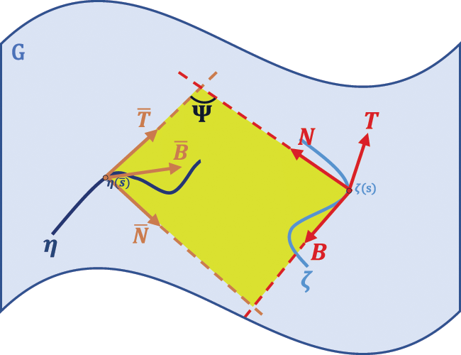
Case 7: We assume that, rectifying plane of the curve ζ is the osculating plane of the curve η, that is Sp{T,B}=Sp{T¯,N¯}. As in Fig. 7, this relationship exists at the corresponding points of along the curves ζ and η.

Figure 7: Rectifying plane of the curve ζ and osculating plane of the curve η

So we have following relation between the curves ζ and η:

η(s¯)=ζ(s)+aT(s)+bB(s),a≠0,b≠0,(51)

where a and b are real valued non-zero functions of s.

Calculating the dot-derivative of the Eq. (51) with the help of Eqs. (3) and (4), we get

T¯(s¯)=(1+a˙−bk0sin⁡α)1rT(s)+(ak0cos⁡α+b(α˙−ϰ0))1rN(s)+(ak0sin⁡α+b˙)1rB(s),(52)

where r=ds¯ds.

We know that N is parallel to B¯, since N⊥=Sp{T,B}=Sp{T¯,N¯}=B¯⊥. If we multiply the Eq. (52) with N, we get

(ak0cos⁡α+b(α˙−ϰ0)1r=0orak0cos⁡α+b(α˙−ϰ0)=0.

And so, we have

T¯(s¯)=(1+a˙−bk0sin⁡α)1rT(s)+(ak0sin⁡α+b˙)1rB(s).(53)

By the Eq. (53), we can set

T¯(s¯)=cos⁡ψ(s)T(s)+sin⁡ψ(s)B(s),N¯(s¯)=−sin⁡ψ(s)T(s)+cos⁡ψ(s)B(s),(54)

where ψ is smooth function between T and T¯ on I and

cos⁡ψ(s)=(1+a˙−bk0sin⁡α)1r,(55)

sin⁡ψ(s)=(ak0sin⁡α+b˙)1r.(56)

By using Eqs. (55) and (56), we obtain

r=(1+a˙−bk0sin⁡α)2+(ak0sin⁡α+b˙)2

and

bk0sin⁡α−a˙+cot⁡ψ(ak0sin⁡α+b˙)=1.

Calculating the dot-derivative of the Eq. (54) with the help of Eqs. (3) and (4), we get

r(k¯0cos⁡α¯N¯+k¯0sin⁡α¯B¯)=(−ψ˙sin⁡ψ−sin⁡ψk0sin⁡α)T+(cos⁡ψk0cos⁡α+sin⁡ψ(α˙−ϰ0))N+(cos⁡ψk0sin⁡α+ψ˙cos⁡ψ)B.(57)

If we multiply the Eq. (57) with N¯ and B¯, respectively, we get

rk¯0cos⁡α¯=ψ˙+kosin⁡α,(58)

rk¯0sin⁡α¯=cos⁡ψk0cos⁡α+sin⁡ψ(α˙−ϰ0).(59)

By using Eqs. (58) and (59), we obtain

ψ˙+kosin⁡α−cot⁡α¯(cos⁡ψk0cos⁡α+sin⁡ψ(α˙−ϰ0))=0.

Thus we introduce the following theorem:

Theorem 3.7. Let ζ:I⊆R→G and η:I¯⊆R→G be two arc-length parametrized curves with the Frenet apparatus {T,N,B,k0,ϰ0,α} and {T¯,N¯,B¯,k¯0,ϰ¯0,α¯}, respectively, in three dimensional Lie group G with left-invariant metric. The rectifying plane of the curve ζ and the osculating plane of the curve η coincide if and only if there exist real valued non-zero functions a and b on I, such that:

ak0cos⁡α+b(α˙−ϰ0)=0,(i)(1+a˙−bk0sin⁡α)2+(ak0sin⁡α+b˙)2≠0,(ii)bk0sin⁡α−a˙+cot⁡ψ(ak0sin⁡α+b˙)=1,(iii)ψ˙+kosin⁡α−cot⁡α¯(cos⁡ψk0cos⁡α+sin⁡ψ(α˙−ϰ0))=0,(iv)

where ψ is the angle between T and T¯ at the corresponding points of ζ and η.

Case 8: We assume that, rectifying plane of the curve ζ is the normal plane of the curve η, that is Sp{T,B}=Sp{N¯,B¯}. As in Fig. 8, this relationship exists at the corresponding points of along the curves ζ and η.

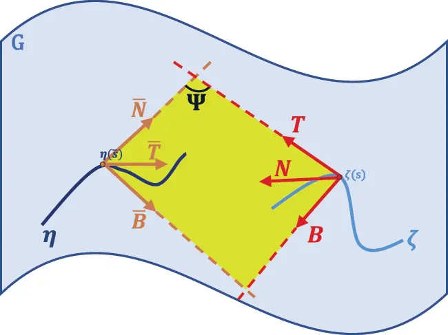
Figure 8: Rectifying plane of the curve ζ and normal plane of the curve η

Thus, we have following relation between the curves ζ and η:

η(s¯)=ζ(s)+aT(s)+bB(s),a≠0,b≠0,(60)

where a and b are real valued non-zero functions of s.

Calculating the dot-derivative of the Eq. (60) with the help of Eqs. (3) and (4), we get

T¯(s¯)=(1+a˙−bk0sin⁡α)1rT(s)+(ak0cos⁡α+b(α˙−ϰ0))1rN(s)+(ak0sin⁡α+b˙)1rB(s),(61)

where r=ds¯ds.

We know that N is parallel to T¯, since N⊥=Sp{T,B}=Sp{N¯,B¯}=T¯⊥. If we multiply the Eq. (61) with T, N and B, respectively, we get

bk0sin⁡α−a˙=1,ak0cos⁡α+b(α˙−ϰ0)=r,ak0sin⁡α+b˙=0.

And so, we have the equation T¯(s¯)=N(s). If we calculate the dot derivative of this equation with the help of Eqs. (3) and (4), we get

r(k¯0cos⁡α¯N¯)+k¯0sin⁡α¯B¯)=(−α˙+ϰ0)B−k0cos⁡αT.(62)

If we multiply the Eq. (62) with N¯(s¯) and B¯(s¯), respectively, we get

rk¯0cos⁡α¯=sin⁡ψ(−α˙+ϰ0)−cos⁡ψk0cos⁡α,(63)

rk¯0sin⁡α¯=cos⁡ψ(−α˙+ϰ0)+sin⁡ψk0cos⁡α,(64)

where ψ is the smooth angle function between the T and N¯. By using Eqs. (63) and (64), we obtain

cot⁡α¯=sin⁡ψ(−α˙+ϰ0)−cos⁡ψk0cos⁡αcos⁡ψ(−α˙+ϰ0)+sin⁡ψk0cos⁡α

that is

sin⁡ψ(−α˙+ϰ0)−cos⁡ψk0cos⁡α−cot⁡α¯(cos⁡ψ(−α˙+ϰ0)+sin⁡ψk0cos⁡α)=0.

Thus we introduce the following theorem:

Theorem 3.8. Let ζ:I⊆R→G and η:I¯⊆R→G be two arc-length parametrized curves with the Frenet apparatus {T,N,B,k0,ϰ0,α} and {T¯,N¯,B¯,k¯0,ϰ¯0,α¯}, respectively, in three dimensional Lie group G with left-invariant metric. The rectifying plane of the curve ζ and the normal plane of the curve η coincide if and only if there exist real valued non-zero functions a and b on I, such that

bk0sin⁡α−a˙=1,(i)ak0cos⁡α+b(α˙−ϰ0)≠0,(ii)ak0sin⁡α+b˙=0,(iii)sin⁡ψ(−α˙+ϰ0)−cos⁡ψk0cos⁡α−cot⁡α¯(cos⁡ψ(−α˙+ϰ0)+sin⁡ψk0cos⁡α)=0,(iv)

where ψ is the angle between T and N¯ at the corresponding points of ζ and η.

Case 9: We assume that, rectifying plane of the curve ζ is the rectifying plane of the curve η, that is Sp{T,B}=Sp{T¯,B¯}. As in Fig. 9, this relationship exists at the corresponding points of along the curves ζ and η.

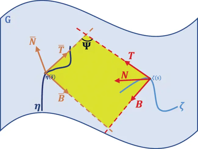
Figure 9: Rectifying planes of the curves ζ and η

Thus, we have following relation between the curves ζ and η:

η(s¯)=ζ(s)+aT(s)+bB(s),a≠0,b≠0,(65)

where a and b are real-valued non-zero functions of s.

Calculating the dot-derivative of the Eq. (65) with the help of Eqs. (3) and (4), we get

T¯(s¯)=(1+a˙−bk0sin⁡α)1rT(s)+(ak0cos⁡α+b(α˙−ϰ0))1rN(s)+(ak0sin⁡α+b˙)1rB(s),(66)

where r=ds¯ds.

We know that N is parallel to N¯, since N⊥=Sp{T,B}=Sp{T¯,B¯}=B¯⊥. If we multiply the Eq. (66) with N, we get

(ak0cos⁡α+b(α˙−ϰ0)1r=0orak0cos⁡α+b(α˙−ϰ0)=0.

And so, we have

T¯(s¯)=(1+a˙−bk0sin⁡α)1rT(s)+(ak0sin⁡α+b˙)1rB(s)(67)

By the Eq. (67), we can set

T¯(s¯)=cos⁡ψ(s)T(s)+sin⁡ψ(s)B(s),B¯(s¯)=−sin⁡ψ(s)T(s)+cos⁡ψ(s)B(s),(68)

where ψ is smooth angle function between T and T¯ on I and

cos⁡ψ(s)=(1+a˙−bk0sin⁡α)1r,(69)

sin⁡ψ(s)=(ak0sin⁡α+b˙)1r.(70)

By using Eqs. (69) and (70), we obtain

r=(1+a˙−bk0sin⁡α)2+(ak0sin⁡α+b˙)2

and

bk0sin⁡α−a˙+cot⁡ψ(ak0sin⁡α+b˙)=1.

Calculating the dot-derivative of the Eq. (68) with the help of Eqs. (3) and (4), we get

r(k¯0cos⁡α¯N¯+k¯0sin⁡α¯B¯)=(−ψ˙sin⁡ψ−sin⁡ψk0sin⁡α)T+(cos⁡ψk0cos⁡α+sin⁡ψ(α˙−ϰ0))N+(cos⁡ψk0sin⁡α+ψ˙cos⁡ψ)B.(71)

If we multiply the Eq. (71) with N¯ and B¯, respectively, we get

rk¯0cos⁡α¯=cos⁡ψk0cos⁡α+sin⁡ψ(α˙−ϰ0),(72)

rk¯0sin⁡α¯=ψ˙+kosin⁡α.(73)

By using Eqs. (72) and (73), we obtain

cos⁡ψk0cos⁡α+sin⁡ψ(α˙−ϰ0)−cot⁡α¯(ψ˙+kosin⁡α)=0.

Thus we introduce the following theorem:

Theorem 3.9. Let ζ:I⊆R→G and η:I¯⊆R→G be two arc-length parametrized curves with the Frenet apparatus {T,N,B,k0,ϰ0,α} and {T¯,N¯,B¯,k¯0,ϰ¯0,α¯}, respectively, in three dimensional Lie group G with left-invariant metric. The rectifying planes of these curves coincide if and only if there exist real valued non-zero functions a and b on I, such that

ak0cos⁡α+b(α˙−ϰ0)=0,(i)(1+a˙−bk0sin⁡α)2+(ak0sin⁡α+b˙)2≠0,(ii)bk0sin⁡α−a˙+cot⁡ψ(ak0sin⁡α+b˙)=1,(iii)cos⁡ψk0cos⁡α+sin⁡ψ(α˙−ϰ0)−cot⁡α¯(ψ˙+kosin⁡α)=0,(iv)

where ψ is the angle between T and T¯ at the corresponding points of ζ and η.

4  Conclusions

It is well known that every smooth curves have a moving Frenet frame. This paper examines the relations between Frenet planes of two smooth curves in three dimensional Lie groups with left-invariant metric. There are nine possible relations that can occur. For each cases, we give conditions by nine theorems as above. These results are generalizations for relations between Frenet planes of two curves in three dimensional Euclidean spaces. By the paper's results, one will be able to investigate of special curve couples in three-dimensional Lie groups with left-invariant metric and correlate their results.

Funding Statement: The author received no specific funding for this study.

Conflicts of Interest: The author declares that he has no conflicts of interest to report regarding the present study.

References

1. Bertrand, J. (1850). Mémoire sur la théorie des courbes à double courbure. Journal de Mathématiques Pures et Appliquées, 15, 332-350. [Google Scholar]
2. Matsuda, H., & Yorozu, S. (2003). Notes on bertrand curves. Yokohama Mathematical Journal, 50, 41-54. [Google Scholar]
3. Wang, F., & Liu, H. (2007). Mannheim partner curves in 3-Euclidean space. Mathematics in Practice and Theory, 37, 141-143. [Google Scholar]
4. Çiftçi, U. (2009). A generalization of lancert’s theorem. Journal of Geometry and Physics, 59, 1597-1603. [Google Scholar] [CrossRef]
5. Okuyucu, O., Gök, I., Yaylı, Y., & Ekmekci, F. (2013). Slant helices in three dimensional Lie groups. Applied Mathematics and Computation, 221, 672-683. [Google Scholar] [CrossRef]
6. Okuyucu, O., Gök, I., Yaylı, Y., & Ekmekci, F. (2017). Bertrand curves in three dimensional Lie groups. Miskolc Mathematical Notes, 17(2), 999-1010. [Google Scholar] [CrossRef]
7. Gök, I., Okuyucu, O., Ekmekci, F., & Yaylı, Y. (2014). On mannheim partner curves in three dimensional Lie groups. Miskolc Mathematical Notes, 15(2), 467-479. [Google Scholar] [CrossRef]
8. Yampolsky, A., & Opariy, A. (2019). Generalized helices in three-dimensional Lie groups. Turkish Journal of Mathematics, 43, 1447-1455. [Google Scholar] [CrossRef]
9. Kızıltuğ, S., & Önder, M. (2015). Associated curves of frenet curves in three dimensional compact Lie group. Miskolc Mathematical Notes, 16(2), 953-964. [Google Scholar] [CrossRef]
10. Çakmak, A. (2019). New type direction curves in 3-dimensional compact Lie group. Symmetry, 11(3), 387. [Google Scholar] [CrossRef]
11. Yoon, D., & Yüzbaşı, Z. (2021). A generalization for surfaces using a line of curvature in Lie group. Hacettepe Journal of Mathematics and Statistics, 50(2), 444-452. [Google Scholar] [CrossRef]
12. Bozkurt, Z., Gök, I., Okuyucu, O., & Ekmekci, F. (2013). Characterizations of rectifying, normal and osculating curves in three dimensional compact Lie groups. Life Science Journal, 10(3), 819-823. [Google Scholar] [CrossRef]
13. Karakuş, S., İlarslan, K., & Yaylı, Y. (2014). A new approach for characterization of curve couples in Euclidean 3-space. Honam Mathematical Journal, 36(1), 113-129. [Google Scholar] [CrossRef]
14. Milnor, J. (1976). Curvatures of left invariant metrics on Lie groups. Advances in Mathematics, 21, 293-329. [Google Scholar] [CrossRef]

This work is licensed under a Creative Commons Attribution 4.0 International License, which permits unrestricted use, distribution, and reproduction in any medium, provided the original work is properly cited.