Computer Modeling in Engineering & Sciences

---

DOI: 10.32604/cmes.2022.022103

ARTICLE

Some Properties of Degenerate r-Dowling Polynomials and Numbers of the Second Kind

Hye Kyung Kim1,* and Dae Sik Lee2

1Department of Mathematics Education, Daegu Catholic University, Gyeongsan, 38430, Korea
2School of Electronic and Electric Engineering, Daegu University, Gyeongsan, 38453, Korea
*Corresponding Author: Hye Kyung Kim. Email: hkkim@cu.ac.kr
Received: 21 February 2022; Accepted: 11 May 2022

1  Introduction

The Stirling number S2(n,k) of the second kind counts the number of partitions of the set {1,2,…,n} into k-nonempty disjoint set. The Bell polynomials Bn(x) are given by Bn(x)=∑k=0nS2(n,k)xk, (see [1]).

When x=1, Bn=Bn(1) are called the Bell numbers. The Stirling number S1(n,k) of the first kind counts the number of having permutations of the set {1,2,…,n} having k disjoint cycles.

Dowling [2] constructed a certain lattice for a finite group of order m, called Dowling lattice, and using the Möbius function, he introduced the corresponding Whitney numbers of the first kind wm(n,k) and Whitney numbers of the second kind Wm(n,k)(0≤k≤n,m≥1), which are independent of the group itself, but depend only on its order. For the trivial group, we have w1(n,k)=S1(n+1,k+1) and W1(n,k)=S2(n+1,k+1). Benoumhani [3,4] gave a detailed description of properties of these numbers.

For x∈R, the falling factorials (x)n are given by (x)n=x(x−1)⋯(x−n+1),(n≥1)and(x)0=1, (see [1]).

As a generalization of the the Whitney numbers wm(n,k) and Wm(n,k) of the first and second kind associated with Qn(G), respectively, Mezö [5] introduced r-Whitey numbers of the first and second kind given by

mn(x)n=∑k=0nwm,r(n,k)(mx+r)k,

and

(mx+r)n=∑k=0nWm,r(n,k)mk(x)n,(1)

respectively, for n≥k≥0. And wm,r(0,0)=1 and Wm,r(0,0)=1.

When r=1, wm(n,k)=wm,1(n,k) and Wm(n,k)=Wm,1(n,k).

We note that

w1,0(n,k)=S1(n,k),  W1,0(n,k)=S2(n,k)w1,r(n,k)=S1(n+r,k+r),  W1,r(n,k)=S2(n+r,k+r)wm,1(n,k)=wm(n,k),  Wm,1(n,k)=Wm(n,k).

Note that the r-Whitney numbers of the second kind are exactly the same numbers defined by Ruciński and Voigt et al. [6] and the (r,β)-Stirling numbers defined by Corcino et al. [7].

The r-Whitey numbers of both kinds and r-Dowling polynomials were studied by several authors. The references [2–5,7–15] provided readers more information. In particular, Cheon et al. [8] and Corcino et al. [11] gave combinatorial interpretations of the r-Whitney numbers of the first and second kind, respectively. In recently years, many mathematicians have been studied the degenerate special polynomials and numbers, and have obtained many interesting results [14,16–24]. In particular, the generating functions of (degenerate) special numbers and polynomials have various applications in many fields as well as mathematics and physics [1–32]. Kim et al. [14] introduced the degenerate Whitney numbers of the first kind and the second kind of Dowling lattice Qn(G) of rank n over a finite group G of order m, respectively, as follows:

mn(x)n=∑k=0nwm,λ(n,k)(mx+1)k,λ,(n≥0).(2)

and

(mx+1)n,λ=∑k=0nWm,λ(n,k)mk(x)k,(n≥0),see [14].(3)

With these in mind, we naturally introduce the degenerate r-Dowling polynomials and numbers associated with the degenerate r-Whitney numbers Wm,r(n,k) of the second kind in this paper. We explore various properties and identities for the degenerate r-Dowling polynomials and numbers including generating functions, Dobinski-like formula, integral representations, recurrence relations, various explicit expressions. Furthermore, we investigate several expressions for them that can be derived from repeated applications of certain operators to the exponential functions, the derivatives of them and some identities involving them.

2  Preliminaries

In this section, we introduce the basic definitions and properties of the degenerate r-Dowling polynomials and numbers needed in this paper.

For x∈R, the rising factorials ⟨x⟩n are given by ⟨x⟩n=x(x+1)⋯(x+n−1),(n≥1)and⟨x⟩0=1, (see [1]).

Cheon et al. [8] introduced the r-Dowling polynomials associated with the r-Whitney numbers Wm,r(n,k) of the second kind are given by

Dm,r(n,x)=∑k=0nWm,r(n,k)xk,(see[8]).(4)

By (1) and (4), the generating function of r-Dowling polynomials is given by

∑k=0∞Dm,r(n,x)tnn!=exp⁡(rt+xemt−1m),(see [8,11,13]),

where exp⁡(t)=et.

Corcino et al. [11] studied asymptotic formulas for r-Whitney numbers of the second kind with integer and real parameters. They also obtained the range of validity of each formula.

As is well known, for any λ∈R,

eλx(t)=(1+λt)xλ=∑n=0∞(x)n,λtnn!,(|λt|<1),(see [16-24]),(5)

where (x)n,λ=x(x−λ)⋯(x−(n−1)λ))(n≥1) and (x)0,λ=1. When λ→0, eλx(t)=ext.

The degenerate Stirling numbers of the second kind are given by

1k!(eλ(t)−1)k=∑n=k∞S2,λ(n,k)tnn!(k≥0),(see [16,19,22]).(6)

Kim et al. studied the unsigned degenerate r-Stirling numbers of the second kind defined by

(x+r)n,λ=∑j=0nS2,λ(r)(n+r,j+r)(x)j,(n≥0),(see [22]).(7)

From (7), the generating function of the degenerate r-Stirling numbers of the second kind is given by

eλr(t)1j!(eλ(t)−1)j=∑n=j∞S2,λ(r)(n+r,j+r)tnn!,(see [22]).(8)

where j is a non-negative integer.

In view of (8), the degenerate r-Bell polynomials are given by

Beln(r)(x|λ)=∑j=0nS2,λ(r)(n+r,j+r)xj,(n≥0),(see [22]).(9)

From (9), it is easy to show that the generating function of degenerate r-Bell polynomials is given by

eλr(t)ex(eλ(t)−1)=∑n=0∞Beln(r)(x|λ)tnn!,(see [22]).(10)

when x=1, Beln(r)(λ)=Beln(r)(1|λ) are called the degenerate r-Bell numbers.

Kim et al. introduced the λ-binomial coefficients defined as

(xn)λ=(x)n,λn!=x(x−λ)⋯(x−(n−1)λ)n!,(n≥1)and(x0)λ=1(λ∈R),(see [20]).(11)

From (11), we easily get

(x+yn)λ=∑l=0n(xl)λ(yn−l)λ,(n≥0),(see [20]).(12)

From (12), we note that

(x+y)n,λ=∑k=0n(nk)(x)k,λ(y)n−k,λ.(13)

3  Degenerate r-Dowling Polynomials and Numbers

In this section, we explore various properties for the degenerate r-Dowling polynomials and numbers.

From (1), the degenerate r-Whitney numbers Wm,λ(r)(n,k) of the second kind are given by

(mx+r)n,λ=∑k=0nWm,r(n,k)mk(x)n,(see [14]).(14)

Lemma 3.1. [14] For k≥0, we have the generating function of the degenerate r-Whitney numbers of the second kind as follows:

∑n=j∞Wm,r,λ(n,j)tnn!=eλr(t)1j!(eλm(t)−1m)j.

In Lemma 3.1, when r=1, we have the generating function of the degenerate Whitney numbers of the second kind as follows:

∑n=j∞Wm,λ(n,j)tnn!=eλ(t)1j!(eλm(t)−1m)j,(see [16]).

From Lemma 3.1, (6) and (8), we get

W1,r,λ(n,j)=S2,λ(r)(n+r,j+r),W1,0,λ(n,j)=S2,λ(n,j),Wm,1,λ(n,j)=Wm,λ(n,j).(15)

The next theorem is a recurrence relation of the degenerate Whitney numbers of the second kind.

Theorem 3.1. For n≥0, we have

Wm,r,λ(n+1,j)=Wm,r,λ(n,j−1)+(mj+r−nλ)Wm,r,λ(n,j).

Proof. From (14), we observe that

∑j=0n+1Wm,r,λ(n+1,j)mj(x)j=(mx+r)n+1,λ=(mx+r−λn)(mx+r)n,λ=∑j=0nWm,r,λ(n,j)mj(x)j{m(x−j)+mj+r−nλ}=∑j=1n+1Wm,r,λ(n,j−1)mj(x)j+∑j=0nWm,r,λ(n,j)(mj+r−nλ)mj(x)j=∑j=0n+1{Wm,r,λ(n,j−1)+Wm,r,λ(n,j)(mj+r−nλ)}mj(x)j.(16)

By comparing the coefficients of both sides of (16), we get the desired recurrence relation.

The following theorem shows that the degenerate r-Whitney numbers of second kind expresses the finite sum of degenerate falling factorials.

Theorem 3.2. For n,j≥0, we have

1j!mj∑d=0j(jd)(−1)j−d(dm+r)n,λ={Wm,r,λ(n,j)ifn≥j,0ifotherwise.

Proof. By (5) and Lemma 3.1, we observe that

∑n=j∞Wm,r,λ(n,j)tnn!=eλr(t)1j!(eλm(t)−1m)j=1j!mj∑d=0j(jd)(−1)j−d∑n=0∞(dm+r)n,λtnn!=∑n=0∞(1j!mj∑d=0j(jd)(−1)j−d(dm+r)n,λ)tnn!.(17)

By comparing the coefficients of both sides of (17), we get the desired result.

In Theorem 3.2, when r=1, for n≥k≥0, we get

1j!mj∑d=0j(jd)(−1)j−d(dm+1)n,λ={Wm,λ(n,j)ifn≥j,0ifotherwise,(see [14]).

In this paper, we naturally consider the degenerate r-Dowling polynomials of the second kind given by

Dm,r,λ(n|x)=∑j=0nWm,r,λ(n,j)xj,(n≥0).(18)

When x=1, Dm,r,λ(n)=Dm,r,λ(n|1) are called the degenerate r-Dowling numbers of the second kind.

When r=1, Dm,λ(n,x)=Dm,1,λ(n|x) are the degenerate Dowling polynomials in of the second kind [14].

When r=1, the degenerate r-Dowling polynomials of the second kind are different from the fully degenerate Dowling polynomials in [23].

Theorem 3.3. For m∈N, the generating function of degenerate r-Dowling polynomials of the second kind is

eλr(t)ex(eλm(t)−1m)=∑n=0∞Dm,r,λ(n|x)tnn!

Proof. From Lemma 3.1 and (18), we observe that

∑n=0∞Dm,r,λ(n|x)tnn!=∑n=0∞(∑j=0nWm,r,λ(n,j)xj)tnn!=eλr(t)∑j=0∞xj1j!(eλm(t)−1m)=eλr(t)ex(eλm(t)−1m).(19)

By (19), we have the generating function of degenerate r-Dowling polynomials of the second kind.

When m=1, from Theorem 3.3, (10) and (15), we observe that

D1,r,λ(n)=∑j=0nW1,r,λ(n,j)=∑j=0nS2,λ(r)(n+r,j+r)=Beln(r)(λ).

When m=1, r=1 and λ→0, we note that

D1,1(n)=∑j=0nW1,1(n,j)=∑j=0nS2(n+1,j+1).

Theorem 3.4. (Dobinski-like formula)

For n≥0, we have

Dm,r,λ(n|x)=e−xm∑j=0∞(mj+r)n,λj!mjxj,

When r=1, we have

Dm,λ(n|x)=e−1m∑j=0∞(mj+1)n,λj!mjxj.

Proof. From (5) and Theorem 3.3, we note that

∑n=0∞Dm,r,λ(n|x)tnn!=eλr(t)ex(eλm(t)−1m)=e−xm∑j=0∞xj1mjj!eλmj+r(t)=e−xm∑j=0∞xjmjj!∑n=0∞(mj+r)n,λtnn!=∑n=0∞(e−xm∑j=0∞xjmjj!(mj+r)n,λ)tnn!.(20)

By comparing the coefficients of both sides of (20), we have Dobinski-like formula for the degenerate r-Dowling polynomials.

In the following theorem and corollary, we have integral representations of the degenerate r-Whitney numbers and the degenerate r-Dowling polynomials, respectively.

Theorem 3.5. For n,l∈Z with n≥l≥0, we have

Wm,r,λ(n,l)=n!πIm∫02π1l!eλr(eiθ)(eλm(eiθ)−1m)lsin⁡(nθ)dθ,

where i=−1.

Proof. From Lemma 3.1, we get

∫02π1l!eλr(eiθ)(eλm(eiθ)−1m)lsin⁡(nθ)dθ=∑j=l∞Wm,r,λ(j,l)1j!∫02πeijθsin⁡(nθ)dθ=i∑j=l∞Wm,r,λ(j,l)1j!∫02πsin(jθ)sin⁡(nθ)dθ=iπn!Wm,r,λ(n,l).(21)

Therefore, by (21) we have the desired result.

Corollary 3.1. For n≥0, we have

n!πIm∫02πeλr(eiθ)exp⁡(eλm(eiθ)−1m)sin⁡(nθ)dθ=Dm,r,λ(n).

Proof. By Lemma 3.1 and Theorem 3.5, we have

∫02πeλr(eiθ)exp⁡(eλm(eiθ)−1m)sin⁡(nθ)dθ=∑l=0∞∫02πeλr(eiθ)1l!(eλm(eiθ)−1m)lsin⁡(nθ)dθ=∑l=0∞∑j=l∞Wm,r,λ(j,l)1j!∫02πejiθsin⁡(nθ)dθ=i∑j=0∞∑l=0j1j!Wm,r,λ(j,l)∫02πsin(jθ)sin⁡(nθ)dθ=iπn!Dm,r,λ(n).(22)

From (22), we get the desired identity.

Lemma 3.2. For n≥j≥0 and r,m∈N, we have

Wm+1,r,λ(n,j)=1(m+1)jmn−j∑s=0n(ns)(−1)n−s(m+1)s<r>n−s,mλWm,r,mm+1λ(s,j).

Proof. From Theorem 3.2 and (13), we get

Wm+1,r,λ(n,j)=1j!(m+1)j∑l=0j(jl)(−1)j−l(l(m+1)+r)n,λ=(m+1)n−jj!∑l=0j(jl)(−1)j−l(l+rm−rm(m+1))n,λm+1=(m+1)n∑l=0j(jl)(−1)j−l(m+1)jj!∑s=0n(ns)(l+rm)n−s,λm+1(−rm(m+1))s,λm+1=(m+1)n∑s=0n(ns)mj(m+1)jmn−s(−rm(m+1))s,λm+1×1j!mj∑l=0j(jl)(−1)j−l(lm+r)n−s,mm+1λ=(m+1)n∑s=0n(ns)mj(m+1)jmn−s(−1)s(m(m+1))s<r>s,mλWm,r,mm+1λ(n−s,j)=1(m+1)jmn−j∑s=0n(ns)(−1)n−s(m+1)s<r>n−s,mλWm,r,mm+1λ(s,j).(23)

By (23), we obtain the desired result.

The next theorem is a recurrence relation of degenerate r-Dowling polynomials.

Theorem 3.6. For n≥0, we have

Dm+1,r,λ(n|x)=1mn∑j=0n(nj)(−1)n−j(m+1)j<r>n−j,mλDm,r,mm+1λ(j,mm+1x),

Proof. From (18) and Lemma 3.2, we have

Dm+1,r,λ(n|x)=∑j=0nWm+1,r,λ(n,j)xj=∑j=0n(1(m+1)jmn−j∑s=0n(ns)(−1)n−s(m+1)s<r>n−s,mλWm,r,mm+1λ(s,j))xj=1mn∑j=0n(nj)(−1)n−j(m+1)j<r>n−j,mλDm,r,mm+1λ(j,mm+1x).(24)

Here Wm,r,λ(j,d)=0, if d≥j. Thus, by (24), we get what we want.

Theorem 3.7. For n≥j≥0, we have the recursion formula for Wm,r,λ(n,j) as follows:

Wm,r,λ(n+1,j)=n!∑d=j−1n(rWm,r,λ(d,j)+∑c=j−1d(dc)Wm,r,λ(c,j−1)(m)d−c,λ)(−λ)n−dd!.

Proof. For j≥1, from (5) and Lemma 3.1, we observe that

∑n=j−1∞Wm,r,λ(n+1,j)tnn!=ddt1j!eλr(t)(eλm(t)−1m)j=(rj!eλr(t)(eλm(t)−1m)j+1(j−1)!eλr(t)(eλm(t)−1m)j−1eλm(t))11+λt=(∑b=j∞rWm,r,λ(b,j)tbb!+∑l=j−1∞∑c=j−1l(lc)Wm,r,λ(c,j−1)(m)l−c,λtll!)∑i=0∞(−1)iλiti=∑n=j∞∑b=jn(nb)rWm,r,λ(b,j)(n−b)!(−λ)n−btnn!+∑n=j−1∞∑l=j−1n∑c=j−1l(nl)(lc)Wm,r,λ(c,j−1)(m)l−c,λ(n−l)!(−λ)n−ltnn!=∑n=j−1∞(n!∑b=j−1n(rWm,r,λ(b,j)+∑c=j−1b(bc)Wm,r,λ(c,j−1)(m)b−c,λ)(−λ)n−bb!)tnn!.(25)

By comparing the coefficients of both sides of (25), we get what we want.

The following theorem is another recurrence relation of degenerate r-Dowling polynomials.

Theorem 3.8. For n≥0, we have the recurrence formula of Dm,r,λ as follows:

Dm,r,λ(n+1|u)=∑l=0n(nl){r(−λ)n−l(n−l)!+u(m−λ)n−l,λ}Dm,r,λ(l|u).

Proof. From Theorem 3.3, we note that

∂∂teλr(t)exp⁡(ueλm(t)−1m)=∂∂t∑n=0∞Dm,r,λ(n|u)tnn!=∑n=0∞Dm,r,λ(n+1|u)tnn!.(26)

On the other hand, by (26), we get

∂∂teλr(t)exp⁡(ueλm(t)−1m)=reλr−λ(t)exp⁡(ueλm(t)−1m)+ueλr(t)exp⁡(ueλm(t)−1m)eλm−λ(t)=(r∑i=0∞(−λ)ii!tii!+u∑j=0∞(m−λ)j,λtjj!)∑l=0∞Dm,r,λ(l|u)tll!=∑n=0∞∑l=0n(nl)(r(−λ)n−l(n−l)!Dm,r,λ(l|u)+u(m−λ)n−l,λDm,r,λ(l|u))tuu!.(27)

By comparing the coefficients of (26) with (27), we get the desired identity.

Remark. When u=1, we have

Dm,r,λ(n+1)=∑l=0n(nl){r(−λ)n−l(n−l)!+(m−λ)n−l,λ}Dm,r,λ(l).(28)

Next, we explore two identities including degenerate r-Dowling polynomials that can be derived from repeated applications of certain operators to the degenerate exponential functions.

Theorem 3.9. For n≥0, we have

∂n∂tneλr(t)exp⁡(xmeλm(t))=eλr−nλ(t)exp⁡(xmeλm(t))Dm,r,λ(n|xeλm(t)).

Proof. First, we observe that

∂∂teλmj+r(t)=∂∂t(1+λt)mj+rλ=(mj+r)(1+λt)(mj+r)−λλ,∂2∂t2eλmj+r(t)=(mj+r)(mj+r−λ)(1+λt)(mj+r)−2λλ,⋮∂n∂tneλmj+r(t)=(mj+r)n,λeλ−nλ(t)eλmj+r(t).(29)

By (29) and Theorem 3.4,

∂n∂tneλr(t)exm(eλm(t))=∂n∂tn(eλr(t)∑j=0∞xjmjj!eλmj(t))=∑j=0∞xjmjj!(∂n∂tneλmj+r(t))=∑j=0∞xjmjj!(mj+r)n,λeλ−nλ(t)eλmj+r(t)=eλr−nλ(t)∑j=0∞(mj+r)n,λmjj!(xeλm(t))j=eλr−nλ(t)exeλm(t)mDm,λ(n|xeλm(t)).(30)

From (30), we have what we want.

Let An,λ=∑j=0∞(mj+r)n,λj!mj, n=0,1,2,…. From Theorem 3.4, we have Dm,r,λ(n)=e−1mAn,λ.

By Theorem 3.3, we have

∑n=0∞An,λtnn!=e1m∑n=0∞Dm,r,λ(n)tnn!=e1meλr(t)exp⁡(eλm(t)−1m)=eλr(t)exp⁡(eλm(t)m).(31)

From (31), the generating function of An,λ is

eλr(t)exp⁡(eλm(t)m)=∑n=0∞An,λtnn!.(32)

Theorem 3.10. For n≥0, we have

(mu1−λmddu)nurmeuxm=ur−nλmeuxmDm,r,λ(n|u).

Proof. Let eλm(t)=u, Then we have

ddt=dudtddu=(meλm−λ(t))ddu=(mum−λm)ddu.(33)

By (33), we get

(mum−λmddu)nurmexp⁡(xmu)=ur−nλmexp⁡(xmu)Dm,r,λ(n|xu),(n≥0).(34)

By (34), we attain the desired result.

Remark. When x=1, we have

(mu1−λmddu)nurmeum=ur−nλmeumDm,r,λ(n|u).

In Theorem 3.1, when u=1 we observe that

(mum−λmddu)nurmexp⁡(um)|u=1=e1mDn,r,λ(n)=An,λ.(35)

From (35), we obtain A0,λ=e1m and Dm,r,λ(0)=e−1mA0,λ=1.

In (35), when n=1, we get

(mum−λmddu)1urmexp⁡(um)=mum−λm(rmurm−1exp⁡(um)+1murmexp⁡(um))=(r+u)ur−λmeum.(36)

From (36), A1,λ=(r+1)e1m and e−1mA1,λ=(r+1)=Dm,r,λ(1).

In (35), when n=2, we observe that

(mum−λmddu)2urmeum=(mum−λmddu)(r+u)ur−λmeum=mum−λm{ur−λmeum+r−λmur−λ−mm(r+u)eum+1m(r+u)ur−λmeum}=um−r−2λmeum{m+(r−λ)u−1(r+u)+(r+u)}.(37)

From (37), we get

A2,λ=e1m{m+(r−λ)(r+1)+(r+1)}=e1m{m+(r+1)(r−λ+1)}.(38)

Thus, by (38), we have Dm,r,λ(2)=m+(r+1)(r−λ+1).

In the same way, we get

Dm,r,λ(3)=2rλ2+(m−λ)(m−2λ)+(r+1){3m+(r+1)(r+1−3λ)}.(39)

By continuous this process, we get all the r-Dowling numbers Dm,r,λ(n), for n∈N.

As you can see from (39), the larger n, the more difficult it is to calculate by hand. Here we use Mathematica and Fortran language to find these values.

In Fig. 1, when m=5, we can see the change of D5,r,0.1(2) and D5,r,0.5(2) depending on r by using Mathematica (x-axis is the numbers of r, y-axis D(2) is the numbers of D5,r,0.1(2) and D5,r,0.5(2), respectively).

Figure 1: D(2) = D5,r,λ(2), when λ = 0.1 and 0.5, respectively

In Fig. 2, when m=5, we can see the change of D5,r,0.1(3) and D5,r,0.5(3) depending on r by using Mathematica (x-axis is the numbers of r, y-axis D(3) is the numbers of D5,r,0.1(3) and D5,r,0.5(3), respectively).

Figure 2: D(3) = D5,r,λ(3), when λ = 0.1 and 0.5, respectively

In Fig. 3, when λ=0.1, we can see the change of D10,1,0.1(n) and D50,1,0.1(n), respectively, by using Fortran language (x-axis is the numbers of n, y-axis log10(D(n)) is the value of log10 (numbers of D10,1,0.1(n) and D50,1,0.1(n), respectively).

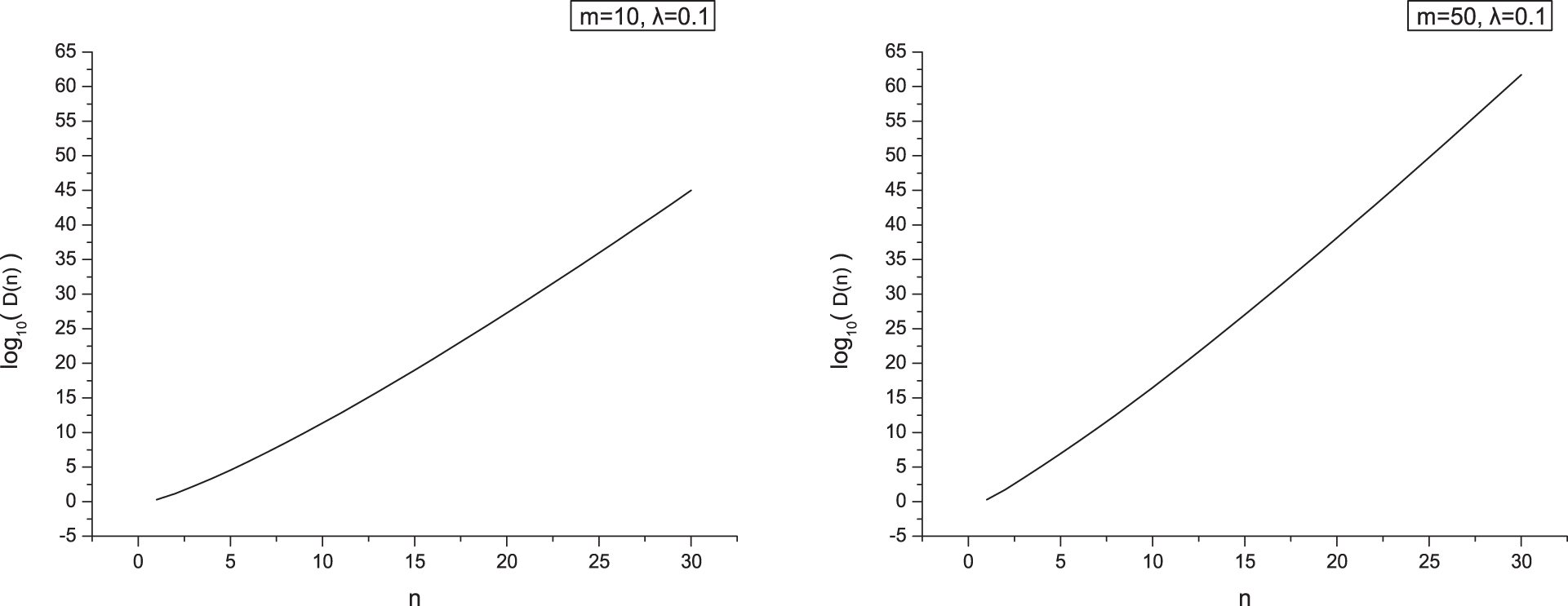
Figure 3: log10(D(n)) = log10(Dm,1,0.1(n)) when m = 10 and 50, respectively

In Fig. 4, when λ=0.5, we can see the change of D10,1,0.5(n) and D50,1,0.5(n), respectively, by using Fortran language (x-axis is the numbers of n, y-axis log10(D(n)) is the value of log10 (numbers of D10,1,0.5(n) and D50,1,0.5(n)), respectively).

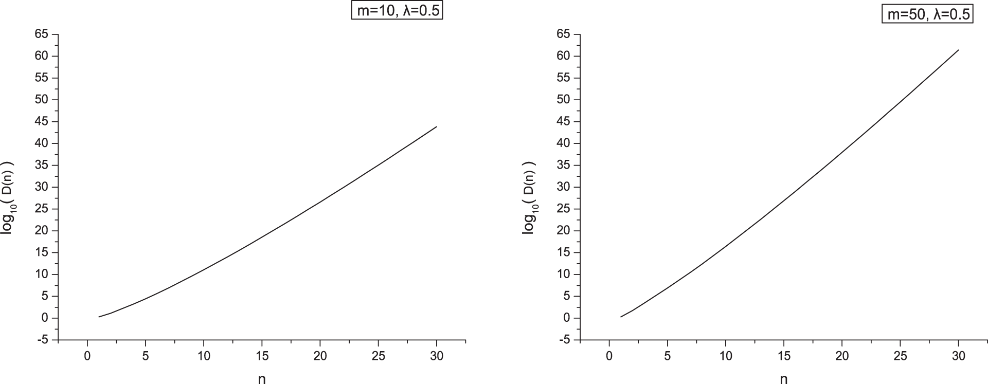
Figure 4: log10(D(n)) = log10(Dm,1,0.5(n)) when m = 10 and 50, respectively

Next, we can get differential equation for degenerate r-Dowling polynomials as follows:

Theorem 3.11. For n≥0, we have

Dm,r,λ(n+1|u)=(u+(r−nλ))Dm,r,λ(n|u)+mudduDm,r,λ(n|u).

Proof. By using Theorem 3.4, we observe

ddu(ur−nλmDm,r,λ(n|u))=ddu(ur−nλmexp⁡(−um)∑j=0∞(mj+r)n,λj!mjuj)=ddu(exp⁡(−um)∑j=0∞(mj+r)n,λj!mju(mj+r)−nλm)=−1mexp⁡(−um)∑j=0∞(mj+r)n,λj!mju(mj+r)−nλm+exp(−um)∑j=0∞(mj+r)n+1,λj!mj+1u(mj+r)−nλmu−1=−1m{ur−nλmDm,r,λ(n|u)−u(r−m)−nλmDm,r,λ(n+1|u)}.(40)

On the other hand, we have

ddu(ur−nλmDm,r,λ(n|u))=r−nλmur−nλ−mmDm,r,λ(n|u)+ur−nλmdduDm,r,λ(n|u).(41)

By (40) and (41), we have

u(r−m)−nλmDm,r,λ(n+1|u)=ur−nλmDm,r,λ(n|u)(1+r−nλu)+ur−nλmmdduDn,r,λ(n|u).(42)

From (42), we get

1uDm,r,λ(n+1|u)=(1+r−nλu)Dm,r,λ(n|u)+mdduDm,r,λ(n|u).(43)

By (43), we obtain the desire result.

Now, we study the derivative of degenerate r-Dowling polynomials Dm,r,λ(n|x).

Theorem 3.12. For n≥1, we have

dduDm,r,λ(n|u)=1m∑l=0n−1(nl)(m)n−l,λDm,r,λ(l|u).

Proof. From (5) and Theorem 3.3, we observe that

∑n=0∞dduDm,r,λ(n|u)tnn!=∂∂u(eλr(t)exp⁡(ueλm(t)−1m))=eλr(t)eλm(t)−1mexp⁡(ueλm(t)−1m)=eλm(t)−1m∑l=0∞Dm,r,λ(l|u)tll!=1m(∑i=0∞(m)i,λtii!−1)∑l=0∞Dm,r,λ(l|u)tll!=1m∑n=0∞(∑l=0n(nl)(m)n−l,λDm,r,λ(l|u)−Dm,r,λ(n|u))tnn!=1m∑n=0∞(∑l=0n−1(nl)(m)n−l,λDm,r,λ(l|u))tnn!.(44)

By comparing the coefficients on both sides of (44), we attain the desired identity.

Theorem 3.13. For n≥1, we have

Dm,r,λ(n|u)=(r)n,λ+∑l=0n−1(nl)(n)n−l,λ∫0uDm,r,λ(l|u)du.

Proof. From (5) and Theorem 3.3, we have

∑n=0∞∫0uDm,r,λ(n|u)dutnn!=∫0ueλr(t)exp⁡(ueλm(t)−1m)du=eλr(t)∫0uexp(ueλm(t)−1m)du=eλr(t)meλm(t)−1[exp⁡(ueλm(t)−1m)]0u.(45)

From (45), we observe that

(eλm(t)−1)∑l=0∞∫0uDm,r,λ(l|u)dutll!=eλr(t){exp⁡(ueλm(t)−1m)−1}.(46)

By (46), we have

∑j=1∞(m)j,λtjj!∑l=0∞∫0uDm,r,λ(l|u)dutll!=∑n=0∞Dm,r,λ(n|u)tnn!−∑n=0∞(r)n,λtnn!.(47)

From (47), we obtain

∑n=1∞∑l=0n−1(nl)(m)n−l,λ∫0uDm,r,λ(l|u)dutnn!=∑n=0∞{Dm,r,λ(n|u)−(r)n,λ}tnn!.(48)

By comparing the coefficients of both sides of (45), we have the desired identity.

If we put y=uq(q∈N∪{0}) and apply the next theorem, we get another interesting identity depending on the variable q different from Theorem 3.10.

Theorem 3.14. For n≥0, we have the operational formula as follows:

(mu1−λmddu)nuqrmexp⁡(uqm)=qnurq−nλmexp⁡(uqm)Dm,r,λq(n|uq).

Proof. Let y=uq(q∈N∪{0}). Then we have

mu1−λmddu=mu1−λmquq−1ddy=mym−λmqqyq−1qddy=mqymq−λmqddy=mqy1−λmqddy.(49)

Thus, by (49), we have

(mu1−λmddu)nuqrmexp⁡(uqm)=qn(my1−λmqddy)nyrmexp⁡(ym)=qnyr−nλqmexp⁡(ym)Dm,r,λq(n|y)=qnurq−nλmexp⁡(uqm)Dm,r,λq(n|uq).(50)

From (50), we attain the desired formula.

4  Conclusion

In this paper, we studied many interesting properties for the degenerate r-Dowling polynomials and numbers associated with the degenerate r-Whitney numbers of the second kind. Among these identity expressions, we obtained the generating function in Theorem 3.3, Dobinski-like formula in Theorem 3.4, recurrence relations in Theorem 3.6 and 3.8, differential equation in Theorem 3.11, the derivatives of them in Theorem 3.12 for r-Dowling polynomials of the second kind. In particular, we obtained some expressions for them that can be derived from repeated applications of certain operators to the exponential functions in Theorem 3.9, 3.10 and 3.14, and some identities involving integration in Theorem 3.13. Furthermore, we found that all exact values of all r-Dowling numbers of the second kind can be obtained using (28). As a follow-up study of this paper, we can explore truncated degenerate r-Dowling polynomials and degenerate r-Dowling polynomials arising from λ-Sheffer sequences. Hence, for future projects, we would like to conduct research into some potential applications of r-Dowling polynomials of the first and second kind, respectively.

Acknowledgement: The author would like to thank the referees for the detailed and valuable comments that helped improve the original manuscript in its present form. Also, the authors thank Jangjeon Institute for Mathematical Science for the support of this research.

Authors’ Contributions: HKK structured and wrote the whole paper. DSL performed computer simulations in the paper. All authors checked the results of the paper and completed the revision of the article.

Consent for Publication: The authors want to publish this paper in this journal.

Ethics Approval and Consent to Participate: The authors declare that there is no ethical problem in the production of this paper.

Funding Statement: This work was supported by the Basic Science Research Program, the National Research Foundation of Korea (NRF-2021R1F1A1050151).

Conflicts of Interest: The authors declare that they have no conflicts of interest to report regarding the present study.

References

 1.  Comtet, L. (1974). Advanced combinatorics: The art of finite and infinite expansions. Dordrecht: Reidel. [Google Scholar]

 2.  Dowling, T. A. (1973). A class of gemometric lattices bases on finite groups. Journal of Combinatorics Theory Series B, 14, 61–86. DOI 10.1016/S0095-8956(73)80007-3. [Google Scholar] [CrossRef]

 3.  Benoumhani, M. (1996). On Whitney numbers of Dowling lattices. Discrete Mathathematics, 159, 13–33. DOI 10.1016/0012-365X(95)00095-E. [Google Scholar] [CrossRef]

 4.  Benoumhani, M. (1997). On some numbers related to Whitney numbers of Dowling lattices. Advanced Applied Matathematics, 19, 106–116. DOI 10.1006/aama.1997.0529. [Google Scholar] [CrossRef]

 5.  Mezö, I. (2010). A new formula for the Bernoulli polynomials. Results Mathmathematics, 58, 329–335. DOI 10.1007/s00025-010-0039-z. [Google Scholar] [CrossRef]

 6.  Ruciński, A., Voigt, B. (1990). A local limit theorem for generalized Stirling numbers. Revue Roumaine de Mathématiques Pures et Appliquées, 35(2), 161–172. [Google Scholar]

 7.  Corcino, R. B., Corcino, C. B., Aldema, R. (2006). Asymptotic normality of the (r, β)-Stirling numbers. Ars Combinbinatorics, 81, 81–96. [Google Scholar]

 8.  Cheon, G. S., Jung, J. H. (2012). r-Whitney numbers of dowling lattices. Discrete Mathematics, 312(15), 2337–2348. DOI 10.1016/j.disc.2012.04.001. [Google Scholar] [CrossRef]

 9.  Cillar, J. A. D., Corcino, R. B. (2020). A q-analogue of Qi formula for r-Dowling numbers. Communications of the Korean Mathematical Society, 35(1), 21–41. DOI 10.4134/CKMS.c180478. [Google Scholar] [CrossRef]

10. Cheon, G. S., El-Mikkawy, M. E. A. (2008). Generalized harmonic numbers with Riordan arrays. Journal of Number Theory, 128, 413–425. DOI 10.1016/j.jnt.2007.08.011. [Google Scholar] [CrossRef]

11. Corcino, C. B., Corcino, R. B., Acala, N. (2014). Asymptotic estimates for r-Whitney numbers of the second kind. Journal of Applied Mathematics, 2014(2), 1–7. DOI 10.1155/2014/354053. [Google Scholar] [CrossRef]

12. Gyimesi, E., Nyul, G. (2018). A comprehensive study of r-Dowling polynomials. Aequationes Mathematics, 92(3), 515–527. DOI 10.1007/s00010-017-0538-z. [Google Scholar] [CrossRef]

13. Gyimesi, E., Nyul, G. (2019). New combinatorial interpretations of r-Whitney and r-Whitney-Lah numbers. Discrete Applied Mathematics, 255, 222–233. DOI 10.1016/j.dam.2018.08.020. [Google Scholar] [CrossRef]

14. Kim, T., Kim, D. S. (2021). A study on degenerate Whitney numbers of the first and second kinds of dowling lattices. arXiv:2013.08904, 22. (To appear Russian Journal of Mathematical Physics). DOI 10.48550/arXiv.2103.08904. [Google Scholar] [CrossRef]

15. Simsek, Y. (2013). Generating functions for generalized Stirling type numbers, array type polynomials, Eulerian type polynomials and their applications. Fixed Point Theory and Applications, 2013, 87. DOI 10.1186/1687-1812-2013-87. [Google Scholar] [CrossRef]

16. Carlitz, L. (1979). Degenerate Stirling, Bernoulli and Eulerian numbers. Utilitas Mathematica, 15, 51–88. [Google Scholar]

17. Lee, C. J., Kim, D. S., Kim, H., Kim, T., Lee, H. (2021). Study of degenerate poly-Bernoulli polynoials by λ-Umbral calculus. Computer Modeling in Engineering & Sciences, 129(1), 393–408. DOI 10.32604/cmes.2021.016917. [Google Scholar] [CrossRef]

18. Kim, D. S., Kim, T. (2020). A note on a new type of degenerate Bernoulli numbers. Russian Journal of Mathematical Physics, 27(2), 227–235. DOI 10.1134/S1061920820020090. [Google Scholar] [CrossRef]

19. Kim, T. (2017). A note on degenerate Stirling polynomials of the second kind. Proceeding of Jangjeon Mathematical Society, 20(3), 319–331. DOI 10.48550/arXiv.1704.02290. [Google Scholar] [CrossRef]

20. Kim, T., Kim, D. S., Lee, H., Kwon, J. (2020). Degenerate binoial coefficients and degenerate hypergeometric functions. Advances in Difference Equations, 2020(115), 17. DOI 10.1186/s13662-020-02575-3. [Google Scholar] [CrossRef]

21. Kim, T., Kim, D. S., Lee, H., Park, S., Kwon, J. (2021). New properties on degenerate Bell polynomials. Complexity, 2021, 13. DOI 10.48550/arXiv.2108.06260. [Google Scholar] [CrossRef]

22. Kim, T., Kim, D. S., Lee, H., Park, J. W. (2020). A note on degenerate r-Stirling numbers. Journal of Inequalities and Applications, 2020(4), 521–531. DOI 10.1186/s13660-020-02492-9. [Google Scholar] [CrossRef]

23. Ma, Y., Kim, T., Lee, H., Kim, D. S. (2021). Some identities of fully degenerate dowling and fully degenerate Bell polynomials arising from λ-umbral calculus. arXiv:2108.11090v1. DOI 10.48550/arXiv.2108.11090. [Google Scholar] [CrossRef]

24. Muhiuddin, G., Khan, W. A., Muhyi, A., Al-Kadi, D. (2021). Some results on type 2 degenerate poly-fubini polynomials and numbers. Computer Modeling in Engineering & Sciences, 129(2), 1051–1073. DOI 10.32604/cmes.2021.016546. [Google Scholar] [CrossRef]

25. Wania, A., Choi, J. S., (2022). Truncated exponential based Frobenius-Genocchi and truncated exponential based Apostol type Frobenius-Genocchi polynomials. Montes Taurus Journal of Pure Applied Mathematics, 4(1), 85–96. [Google Scholar]

26. Broder, A. Z. (1984). The r-Stirling numbers. Discrete Mathematics, 49, 241–259. DOI 10.1016/0012-365X(84)90161-4. [Google Scholar] [CrossRef]

27. Cvijoveć, D. (2011). New identities for the partial Bell polynomials. Applied Mathematics Letters, 24, 1544–1547. DOI 10.1016/j.aml.2011.03.043. [Google Scholar] [CrossRef]

28. Kim, D. S., Kim, T., Jang, L. C., Kim, H. K., Kwon, J. (2022). Arithmetic of Sheffer sequences arising from Riemann, Volkenborn and Kim integrals. Montes Taurus Journal of Pure and Applied Mathematics, 4(1), 149–169. [Google Scholar]

29. Kim, T., Kim, D. S. (2020). A note on central Bell numbers and polynomials. Russian Journal of Mathematical Physics, 27(1), 76–81. DOI 10.1134/S1061920820010070. [Google Scholar] [CrossRef]

30. Kim, T., Kim, D. S., Dolgy, D. V., Lee, S., Kwon, J. (2021). Some identities of the higher-order type 2 Bernoulli numbers and polynomials of the second kind. Computer Modeling in Engineering & Sciences, 128(3), 1121–1132. DOI 10.32604/cmes.2021.016532. [Google Scholar] [CrossRef]

31. Simsek, Y. (2019). Explicit formulas for p-adic integrals: Approach to p-adic distributions and somed families of special numbers and polynomials. Montes Taurus Journal of Pure and Applied Mathematics, 1(1), 1–76. DOI 10.48550/arXiv.1910.09296. [Google Scholar] [CrossRef]

32. Kim, T., Kim, D. S., Jang, L. C., Lee, H., Kim, H. (2022). Representations of degenerate Hermite polynomials. Advances in Applied Mathematics, 139, 102359. DOI 10.1016/j.aam.2022.102359. [Google Scholar] [CrossRef]