Computer Modeling in Engineering & Sciences

---

DOI: 10.32604/cmes.2022.021011

ARTICLE

Structural Optimization of Metal and Polymer Ore Conveyor Belt Rollers

João Pedro Ceniz, Rodrigo de Sá Martins, Marco Antonio Luersen* and Tiago Cousseau

Department of Mechanical Engineering, Federal University of Technology–Parana (UTFPR), Curitiba, 81280-340, Brazil
*Corresponding Author: Marco Antonio Luersen. Email: luersen@utfpr.edu.br
Received: 23 December 2021; Accepted: 23 March 2022

Nomenclature

DOE	Design of Experiments
FEA	Finite Element Analysis
GBNM	Globalized Bounded Nelder-Mead
HDPE	High-Density Polyethylene
LHS	Latin Hypercube Sampling
RBF	Radial Basis Functions
Di	Design Variable
f(x)	Objective Function
fp(x)	Penalized Objective Function
f^(x)	Radial Basis Approximation Function
gi(x)	The Value of the Constraint Function Evaluated at the Point x
g¯i	Reference Value of the Constraint
k	Non-Dimensional Exponent
SVM	Maximum von Mises Stress
x	General Point
x(i)	Sampling Point
β	Bearing Misalignment Angle
δi	Penalized Objective Function’s Parameter
ψ	Radial Basis Function Type
ωi	Radial Basis Function Weight
‖.‖	Euclidean Norm

1  Introduction

In several sectors of the economy where products and commodities must be transported continuously, the use of conveyor belts is an excellent choice. Ingale et al. [1] pointed out that conveyors are often used to move materials safely from one place to another, a process that is both time-consuming and expensive when carried out by humans. Conveyor belts depend on the use of several rollers to ensure longitudinal movement of the belt so that the material is transported from one place to another.

However, as noted by Vasić et al. [2], rollers operate in harsh environments in the mining industry, where they are subjected to high loads and temperatures, the effects of the weather and contamination of the bearing lubricants. As a result of these factors, as well as inaccuracies during roller manufacture and assembly and roller misalignment during use, as reported by Zhao et al. [3], a significant number of rollers need to be replaced every year and roller life cycle can vary greatly, making the product prone to premature failure. Compounding these problems, rollers are usually made of metal and weigh from 20 to 70 kg each, creating risks for the operator responsible for replacing the product when it is damaged, as this activity is performed manually.

Roller mass can be reduced by using polymer or metals with a lower density than that of steel in the manufacturing process. However, Brazilian standard ABNT NBR 6678.2017 [4], which regulates the requirements for the manufacture and operation of conveyor belt rollers, does not mention recommendations exclusively for rollers produced in materials other than steel, whether polymers or other types of metals. Therefore, when a material other than that recommended by the standard is used, it is the responsibility of the designer to understand the mechanical behavior of the material and carry out the structural design appropriately.

The mechanical behavior of rollers in terms of the stress and strain distributions in the structure can be evaluated using finite element analysis (FEA). By combining FEA and optimization techniques, appropriate roller dimensions can be defined, thereby ensuring an acceptable service life with low mass.

According to Christensen et al. [5], there are three types of structural optimization: shape, parametric and topological optimization. Choosing the most appropriate one to use in the design process is essential before starting the optimization procedure. In the first approach, starting from an initial model/geometry we try to find a new geometry by modifying the shape without removing or adding material in regions that change the “topology” of the structure. In parametric optimization, which is used in this work, the shape of the structure is unchanged, i.e., only some dimensions, such as section diameter, length and thickness are modified during the optimization. In topological optimization, the results can be even more remarkable as there is a more significant change in the shape of the structure, i.e., the “topology” (sets of regions with and without material) can be modified.

Several algorithms that can be used in an optimization procedure are mentioned in the literature. According to Arora [6], some examples are the Conjugate Gradient, Modified Newton, Particle Swarm, Simulated Annealing and Genetic algorithms. The choice of which algorithm to use depends on the definition of the problem to be solved. However, as several iterations are generally required to reach an accurate result regardless of the algorithm used, the optimization process may become unfeasible depending on the time required to run each iteration. Jiang et al. [7] therefore suggested the use of surrogate models as an alternative to reduce the computational cost of the optimization.

According to Rodrigues et al. [8], a surrogate model (also called a metamodel) is equivalent to an approximate model that is used to replace an original high-fidelity model. Briefly, a metamodel can be understood as a simplified function that aims to represent an original function but with a lower computational cost. The simplified function is obtained by using a reduced number of responses from the original function. In the present work, for example, each point is equivalent to a different combination of variables (parameters) corresponding to the dimensions of the roller model to be optimized.

Within this context, the present work describes and apply a low-computational-cost optimization methodology for ore conveyor belt roller designs that have been little studied in the literature. The objective of the study is to develop and apply a parametric structural optimization approach to reduce the mass of two models of rollers, one made completely of metal, while the other also has some components made of polymeric material. The variable parameters of the optimization problem (the design variables) are the dimensions of the shaft and external tube.

The optimization framework uses metamodels based on radial basis functions (RBF). The metamodels construction uses the structural responses of finite element simulations of the roller models and the Globalized Bounded Nelder-Mead [9] is employed as the optimizer. The RBF metamodel is iteratively refined using infill points. The optimization methodology is detailed in Subsections 2.3 to 2.5.

2  Ore Conveyor Belt Roller Optimization Procedure

This section introduces some concepts related to conveyor belt rollers, the formulation of the optimization problems and the optimization strategy used.

2.1 Generalities about Ore Conveyor Belt Rollers

Conveyor belt rollers must direct, sustain and/or absorb the impact of loads from conveyor belts loaded with material to be transported. To perform these functions, rollers consist essentially, from a structural point of view, of three types of components: bearings, shaft and external tube.

The bearings are responsible for allowing the tube to rotate, and at the same time they transfer the load from the contact between the tube and conveyor to the shaft. The shaft supports the roller load and is fixed on two supports at its ends that prevent it moving vertically or axially. The external tube (or barrel) is usually made of steel and is the part in contact with the belt.

In some roller models, two tubes can be used, as shown in Fig. 1. An alternative is to use bearing holders, which hold the bearings in position and are in direct contact with the inner part of the roller, as shown in Fig. 2. The models shown in Figs. 1 and 2 are the rollers that were studied in this work.

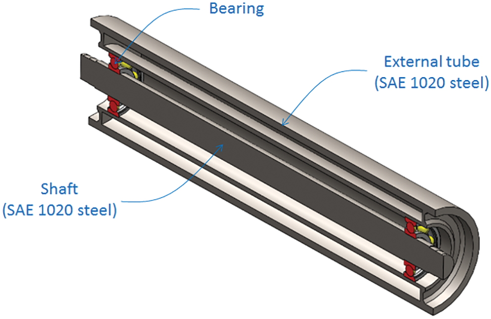
Figure 1: Metal roller (longitudinal section view)

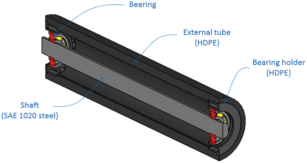
Figure 2: Polymer roller (longitudinal section view)

The current Brazilian standard for the design of this type of mechanical system (ABNT NBR 6678.2017 [4]) classifies rollers according to their use, stipulates the minimum load that must be supported and defines the recommended dimensions and operating conditions. Based on this standard, the two models studied here are classified as load rollers as they are directly responsible for supporting the conveyor belt. Also, according to the standard, they must support at least the loads defined in Table 1. These values are based on the serial number and length of the tube; the serial number refers to the nominal diameter of the shaft, in mm, in the region where the bearings are positioned.

Also according to the standard, the maximum bending stress must be less than 100 MPa, while the bearing misalignment angle when the roller is in operation must be less than 9′ (i.e., 0.15° or 0.0026 rad). Fig. 3 depicts the misalignment angle, represented by β.

Figure 3: Bearing misalignment angle (adapted from [4])

For polymeric materials, a value of 100 MPa for the bending stress becomes impractical because the material's tensile strength is in a much lower range. Hence, it is recommended that a limit value be stipulated according to the literature for the material studied. In the case of high-density polyethylene (HDPE), the polymer used in one of the rollers studied here, the mechanical properties are within the range of values shown in Table 2 according to Peacock [10].

Unlike metals, polymers exhibit behavior that is highly dependent on factors such as mechanical stress, loading time, temperature and molecular structure. In addition, any degradation of the material has a great influence on its mechanical properties. Polymers also exhibit viscoelasticity, according to Cheng et al. [11], which is the result of a combination of viscous behavior, typical of fluids, and elastic behavior, typical of solids.

When the studies by Zhao et al. [12–14] are compared, it is clear that HDPE specimens behave in different ways depending on the type of aging test used. In some cases, the modulus of elasticity increased, making the material more rigid, while the elongation of the samples decreased, characterizing a tendency to embrittlement of the material. Understanding these concepts helps greatly to ensure that finite element simulation represents the real behavior as closely as possible.

2.2 Structural Analysis of the Rollers

According to Hutton [15], the finite element method (FEM) is a computational technique which aims to provide approximate solutions to engineering problems. Basically, the method involves dividing a structure into several elements connected to each other by points known as nodes. The problem is then solved numerically, attributing an interpolation function to the variable of interest in each of these elements.

Here, the Ansys commercial code was used to build the finite element model, and the corresponding analyses during the optimization process followed the ABNT NBR 6678.2017 standard [4]. As in Berto et al. [16], it was decided to analyze a quarter of the geometry, obtained by separating the roller model in two planes of symmetry. As shown in Fig. 4, there are two cutting planes, for which the corresponding sections are highlighted in orange, one longitudinal and the other transverse.

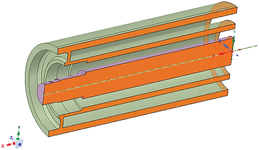
Figure 4: Model of a roller considering two planes of symmetry (bearings and bearing housings are not shown)

The region where the load is applied was determined using the Hertz equations available in Johnson [17]; a conservative higher stress scenario was assumed, and the hyperelastic behavior of the belt material was not taken into account. Despite the real problem presenting dynamic loads, a uniformly distributed load statically applied along the contact area was considered. As the design is based on the guidelines of a standard code for static considerations, this assumption is used in the optimization procedure.

The bearings were represented as spring components whose stiffness was calculated with the equations provided by Gargiulo [18]. The bearings used in the real metal and polymer rollers are SKF model 6309-2Z and 6310-2Z rollers, respectively. Table 3 gives the values of the properties used to perform the numerical simulations for both the metal and polymer (HDPE) rollers.

The von Mises stress distribution and the angle β were obtained by numerical simulation. The latter was calculated using the difference between the displacements of the upper and lower raceways of the bearing. The von Mises stress distribution for the initial design of the metal roller can be seen in Fig. 5.

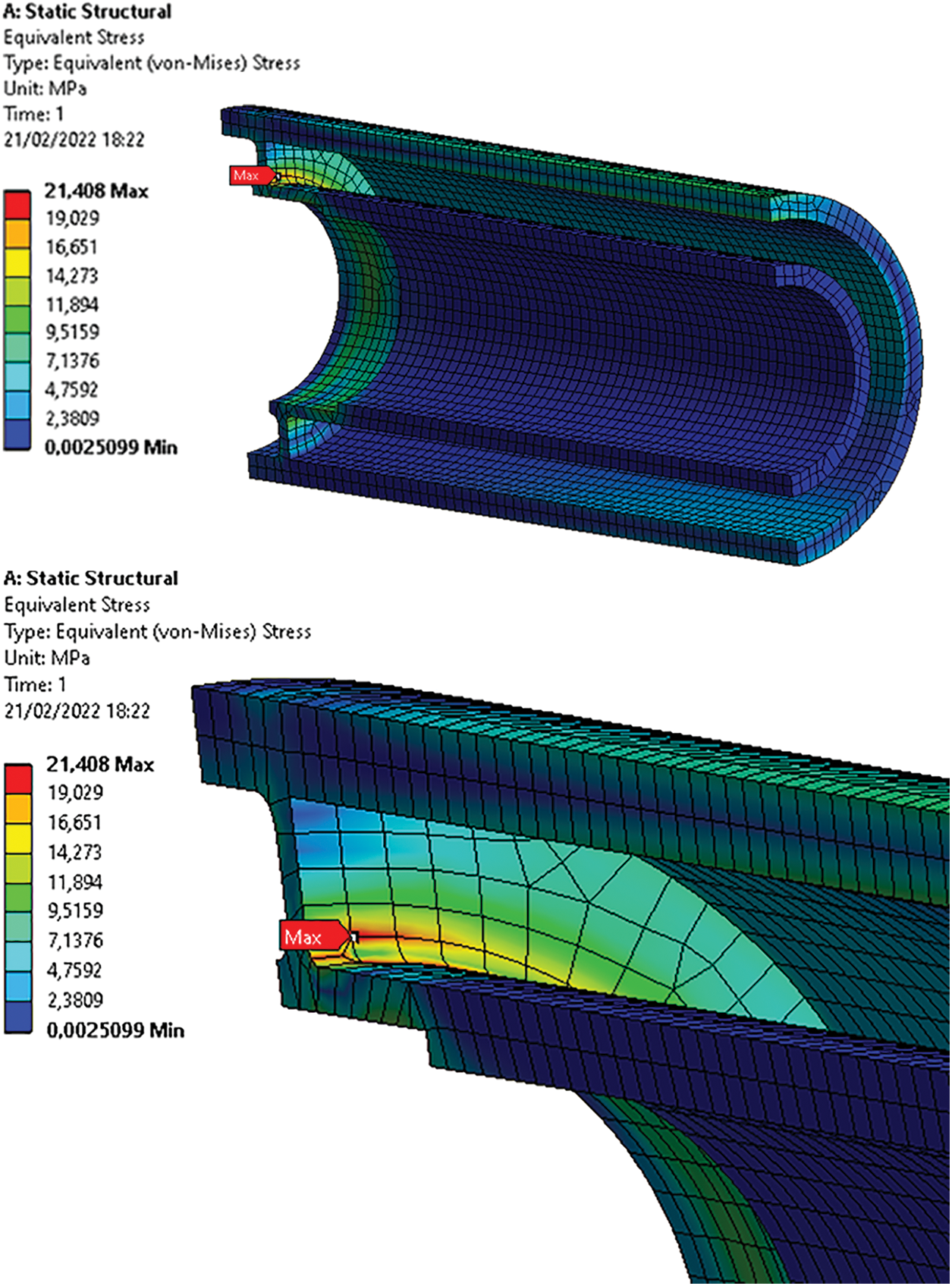
Figure 5: Von Mises stress distribution in the metal roller (initial design)

For each iteration during the optimization process, a static analysis simulation was performed. In the case of the roller with components made of polymeric material, the effects of viscoelasticity were not taken into account as there would be no certainty about how aging would affect the properties of the material. Furthermore, the simulation time would be much longer if viscoelasticity were taken into account, making the optimization unfeasible.

The numerical model was built predominantly with hexahedral (“brick”) quadratic solid finite elements with an average size of 6 mm. This size was determined in a mesh convergence study and provided acceptable accuracy. Figs. 6 and 7 show the finite element meshes for the rollers.

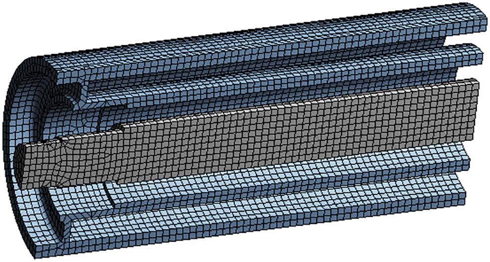
Figure 6: Finite element mesh for the metal roller (the bearings are modeled as a spring element and are not shown)

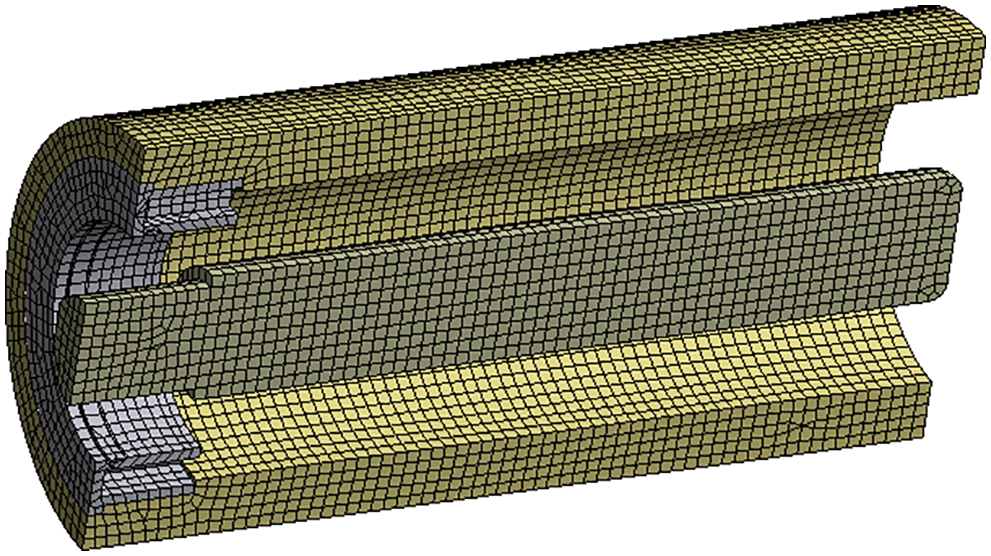
Figure 7: Finite element mesh for the polymer roller (the bearings are modeled as a spring element and are not shown)

2.3 Structural Optimization

According to Arora [6], an optimization problem is mathematically defined as the minimization or maximization of an objective function, which may be subject to equality and/or inequality constraints. The objective function depends on the design variables and, in the context of a structural optimization, can represent the mass or volume of an object, while the variables can represent the dimensions of the object. The design constraints, which can be allowable stresses or displacements or maximum and minimum values of variables, stipulate boundaries that must be respected to make the design feasible.

After the optimization problem has been defined, an optimization method/algorithm should be used to find the best feasible solution. The choice of optimization algorithm is directly related to the definition of the problem. According to Wetter et al. [19], optimization methods can be classified as deterministic (direct search and gradient-based algorithms) or probabilistic. In gradient-based algorithms, calculations of the derivatives (gradient) are needed, so this type of algorithm has limitations when the objective function is discontinuous and/or non-differentiable [20]. Gradient-based algorithms may also get stuck in a local optimum. While direct searches and probabilistic methods do not need gradients, the latter, which are usually based on populations of points, require a large number of simulations to reach convergence, and the former, like gradient-based algorithms, may stop in local optima.

In this work, the Globalized Bounded Nelder-Mead (GBNM) algorithm, proposed by Luersen et al. [9], was used. The GBNM method is a hybrid method that consists of an improved form of the traditional direct search Nelder-Mead algorithm [21] combined with a probabilistic restart, making it a global method if there are enough objective function evaluations.

In an optimization procedure, several iterations are usually required to obtain an appropriate solution. If for each iteration a numerical simulation is performed, obtaining a suitable solution can take several hours. In order to make this process more agile and still robust, one alternative is to apply the optimization algorithm to a surrogate model, which is obtained from a reduced number of simulations and is used as a substitute for the objective function.

2.4 Surrogate Modeling

A surrogate model (or metamodel) can be understood as a simplified representation obtained by regression of the responses of a detailed model or of physical experiments. Here, the surrogate model is an approximate function used to represent a computationally expensive model. In the literature, many types of metamodels for engineering applications can be found, including polynomial regressions, kriging, radial basis functions (RBFs) and artificial neural networks. RBFs are used in this work. As observed by Jin et al. [22] and Hussain et al. [23], the major advantage of RBFs is that they adapt well to different types of linear and non-linear problems. Diaz Gautier et al. [24] pointed out that an important application of RBFs is in metamodel-based optimization of high computational cost functions, and it is used in different schemes for practical problems in engineering.

According to Forrester et al. [25], an RBF metamodel corresponds to an interpolation that combines several simple functions, just as in a polynomial model. However, bases are used, which are radially symmetric functions centered on the various points scattered in the domain. The description of the radial basis approximation function f^ is defined by Eq. (1):

f^(x)=ωTψ=∑i=1nωiψ(‖x−x(i)‖),(1)

where ‖x−x(i)‖ is the Euclidean distance between a general point x and the sampling point x(i), which also corresponds to the center of the base. The term ωi corresponds to a weight for each RBF, and its value has an influence on the accuracy of the metamodel. ψ represents the RBF type. In the literature, the following functions are the most commonly used: linear, cubic, spline, Gaussian, multi quadratic or inverse multi quadratic. The function type that fits best depends on the nature of the problem. Here, cubic functions were used, where ψ is given by Eq. (2):

ψ(r)=r3,(2)

where r=‖x−x(i)‖.

As already mentioned, a metamodel is built from sampling points, which are created in a step known as Design of Experiments (DOE). There are several ways to determine the initial distribution of these points in the design domain, and the choice of technique has a great influence on the accuracy of the metamodel [26,27]. Possible sampling techniques include orthogonal array, full factorial, Sobol sequence and Latin hypercube sampling. The technique selected in this work was Latin hypercube sampling (LHS). According to Forrester et al. [25], samples generated by LHS are organized so that there is only a single orthogonal projection on the axes of each point evaluated.

Even when DOE techniques are used to distribute the sampling points, this does not guarantee that the design space will be adequately represented. This problem becomes even more evident when there is a large number of variables, and as observed by Mack et al. [28], the larger the design space, the more difficult it is to fill. As an alternative, new points (called infill points) can be added at the end of each iteration in order to reduce the number of empty spaces and refine the metamodel [25,29–31]. The infill strategy used here is described in Subsection 2.5.

2.5 Problem Definition and Overview of the Optimization Procedure

The definition of the optimization problem for the metal roller design can be written as Eq. (3):

{Minimize {Mass (D1,D2,D3,D4)}Subject to:{134 mm≤D1≤168 mm110 mm≤D2≤131.6 mm87 mm≤D3≤91 mm54 mm≤D4≤63 mmSVM≤100 MPaβ≤9′,(3)

where Di are the design variables, which can be seen in Fig. 8, SVM represents the maximum von Mises stress and β the bearing misalignment angle. The values of 100 MPa and 9′ for the constraints are from the ABNT NBR 6678.2017 standard [4]. The design variables are chosen in order to not modify the conceptual design of the roller, thus the design found in the optimization process can be used as a part of the mechanical system already installed in the industrial plant.

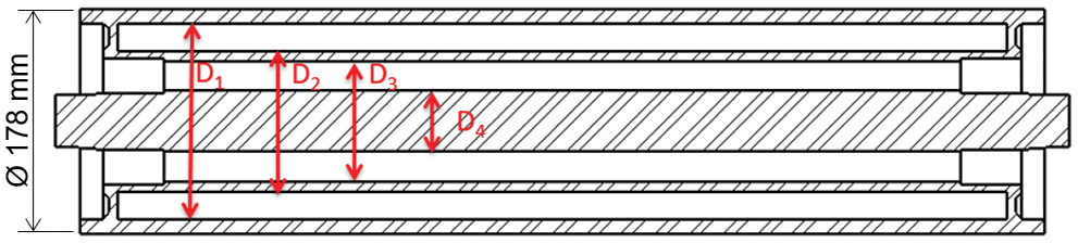
Figure 8: Design variables for the metal roller

For the polymer roller, only two design variables were used (see Fig. 9), and the value of the allowable von Mises stress was defined based on Peacock [10] using a safety factor of 1.5. The same safety factor was imposed on the β angle to make the design more applicable from a practical point of view since degradation of the material is not considered during the simulations. The definition of the optimization problem for the polymer roller can therefore be written as Eq. (4):

{Minimize {Mass (D1,D2)}Subject to:{100 mm≤D1≤150 mm44 mm≤D2≤60 mmSVM≤12 MPaβ≤6′.(4)

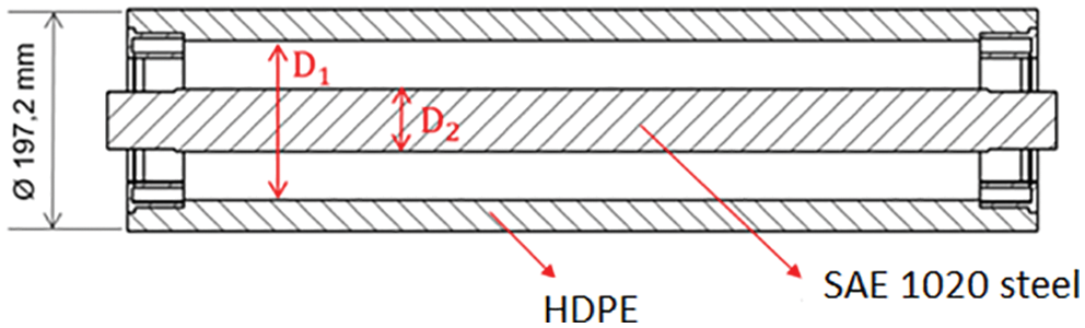
Figure 9: Design variables for the polymer roller

For both rollers, the stress and misalignment angle constraints are handled with a penalty technique, which operates as follows. If for a given point a constraint is violated, the objective function is penalized, making its value higher for that point and decreasing the chances of the point being considered as a candidate for the optimum. The definition of the penalty function, which is added to the objective function if a point is unfeasible, followed the methodology described by Smith et al. [32] with adaptations, giving the Eq. (5):

fp(x)=f(x)+∑i=1m((gi(x)g¯i)k−1)f(x)δi,(5)

where fp(x) is the penalized objective function, f(x) the original objective function (not penalized), m the number of constraints, gi(x) the value of the constraint function evaluated at x, g¯i the reference value of the constraint (for example, for SVM the reference value is 100 MPa for the metal roller), k a non-dimensional exponent defined by the user and δi a parameter which is equal to 1 if the constraint is violated, or null otherwise. In this work, k=1 for the metal roller problem, and k=8 for the polymer roller problem. The choice of an adequate penalization method and the corresponding tuning of its parameters are always critical issues in the constrained optimization problems [33,34]. The values of the exponent k were chosen after some preliminary numerical experiments. A higher k value was used for the polymer roller problem because for this type of roller, optimum design candidates are close to the unfeasible region. A higher penalty should therefore be used to ensure that the constraints will not be violated.

The same optimization strategy is used for both rollers. The GBNM algorithm is used as the optimizer of the RBF metamodel built with the responses of simulations performed on a finite element model in the Ansys software. The metamodel is iteratively refined and optimized.

The steps in the optimization process can be seen in the flowchart in Fig. 10. With the points generated using the LHS methodology, which correspond to different combinations of variables, numerical simulations are performed in Ansys. Thus, the roller masses corresponding to the LHS points are used to build the metamodel of the objective function, while the maximum von Mises stress and bearing misalignment angle define whether or not the penalty function should be activated. The penalized objective function is then optimized using the GBNM algorithm, and one iteration of the proposed methodology is run.

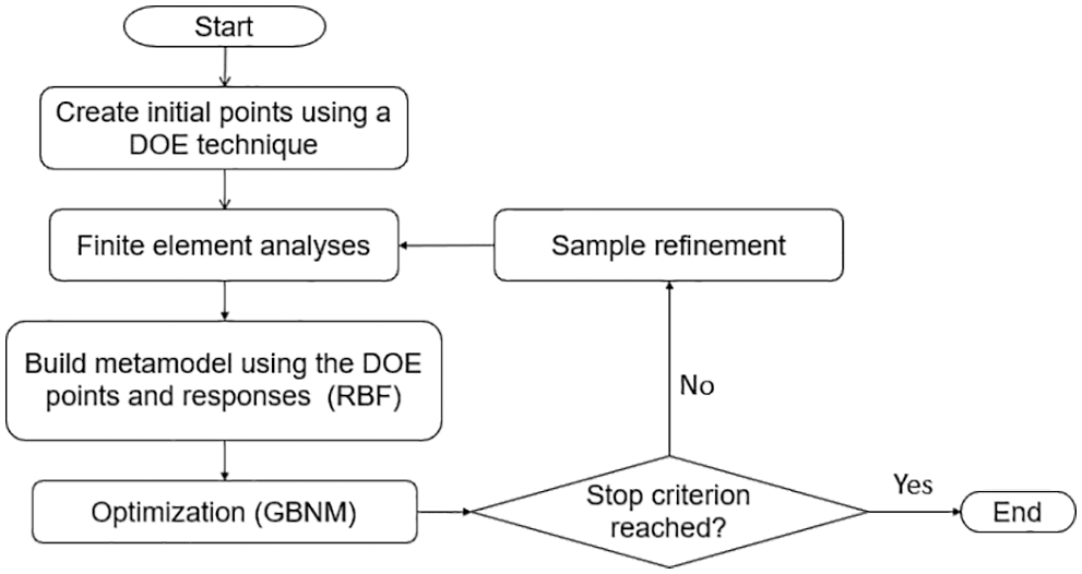
Figure 10: Steps in the optimization process

For the next iteration, two infill points (two new designs and the corresponding responses) are added to the database of the sampling points. The infill points are the minimum found by the GBNM algorithm and a randomly chosen point in the domain. These points (designs) are simulated, and a new metamodel is built. Next, the updated metamodel is optimized again, and two new points (the optimum found by the GBNM algorithm and one randomly chosen point) are then evaluated and used for a new update. These steps are repeated until the previously defined maximum number of evaluations of the objective function (i.e., number of simulations) is reached. Each of these evaluations (simulations) refers to a finite element analysis.

3  Results and Discussion

The optimization of the metal roller was divided into three different cases. The first required 40 simulations (case 1), the second 50 (case 2) and the third 80 (case 3). The simulations and the optimization processes were performed on a computer with an i7–3517U processor and 6 GB of RAM.

Case 1, the original optimization (as presented in Eq. (3)), required approximately 1:56 h and consisted of 30 simulations with DOE sampling points and 10 simulations with infill points.

The other cases served as tests to check the functionality of the penalty function when at least one of the constraints is violated. In case 2, a 60 MPa stress limit was used instead of the 100 MPa constraint, i.e., an additional safety factor was included. Optimization of this case took approximately 2:18 h and used 30 simulations for DOE points and 20 for infill points.

In case 3, instead of the stress constraint, the bearing misalignment angle constraint was checked, and a 5′ limit was imposed instead of the 9′ limit. This optimization required approximately 4:15 h and used 30 simulations for DOE points and 50 for infill points.

As can be observed in many studies reported in the literature (e.g., [35]), there is not a universal rule for the number of points of the initial sample (DOE points). And, since each point represents a simulation, which corresponds to the highest computational cost within an iteration, the total number of points (simulations) usually is limited by the available computational budget. Therefore, the number of DOE points was chosen considering a trade-off between computational cost and space-filling; and the number of infill points considered a trade-off between computational cost and exploration and exploitation of the design space.

The roller mass excluding sealing elements and bearings was 69.14 kg for the initial design and 46.80 kg after optimization in case 1. The evolution of the mass after the DOE simulations can be seen in Fig. 11, where the DOE point with the lowest mass is marked in blue, and the best point after the optimization process is in red.

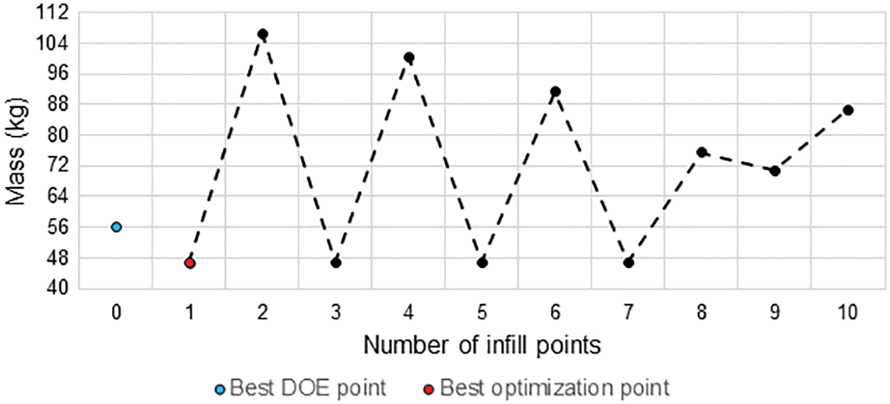
Figure 11: Evolution of the mass of the metal roller during the optimization process (case 1)

The evolution of the stress constraint in the optimization for case 1 after the simulations using each of the DOE points can be seen in Fig. 12, while the evolution of the angle constraint can be seen in Fig. 13. Note that the constraints (stress and angle allowable values) were not violated in any iteration, suggesting the penalization function was not activated during the whole optimization process (the functionality of penalization function is tested in cases 2 and 3). It can be also noted that the best point for case 1 was found in the first iteration (infill point #1), which indicates the problem was quite well represented in the first metamodel, which used only DOE points.

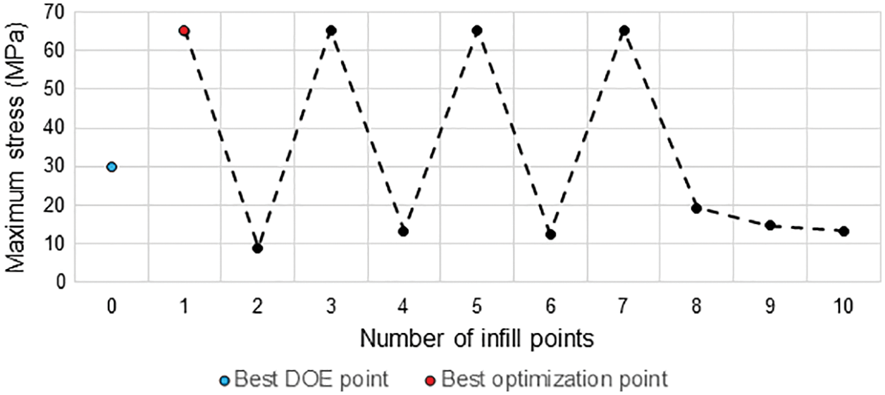
Figure 12: Evolution of the maximum von Mises stress during the optimization process (case 1)

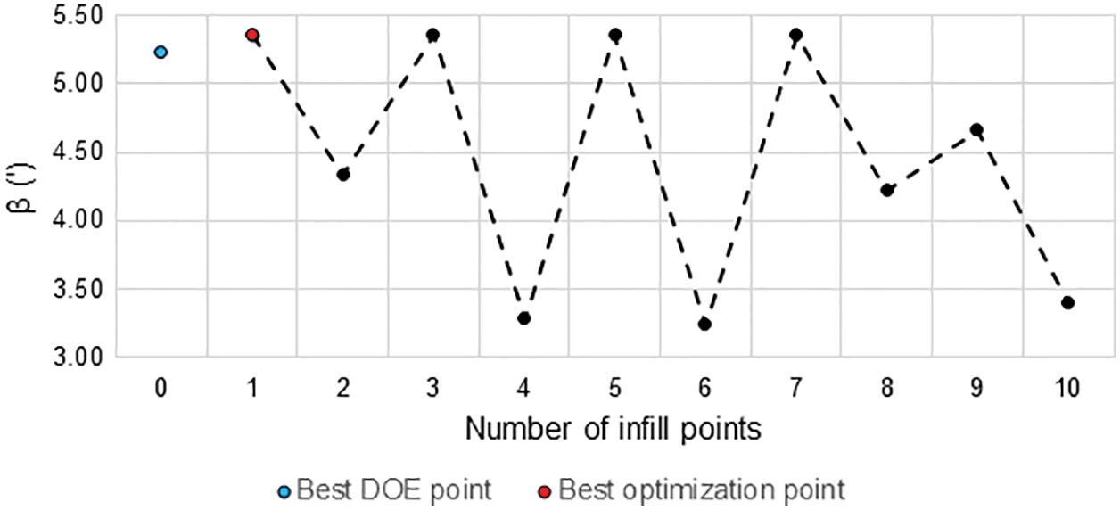
Figure 13: Evolution of the bearing misalignment angle during the optimization process (case 1)

The values obtained for the final configuration of the roller and the initial version, as well as the corresponding percentage variations, are shown in Table 4. The masses of the different versions of the roller do not include the masses of the bearings and labyrinth seal components.

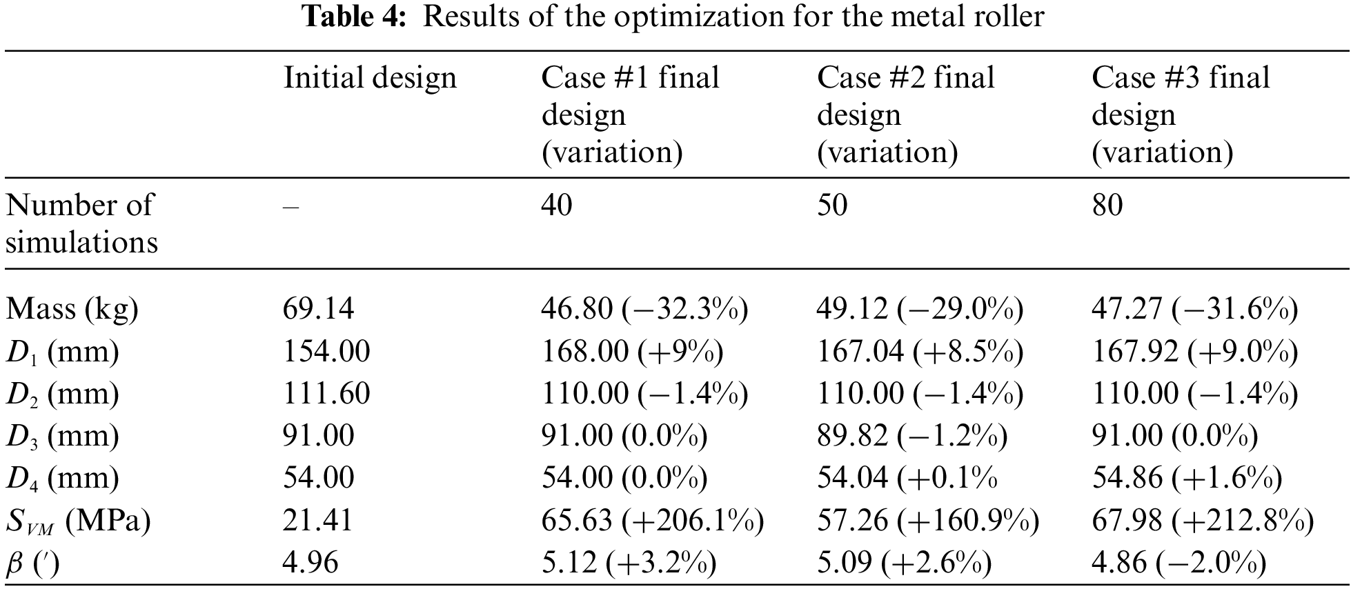
With the optimization, a reduction in roller mass of approximately 32% for the standard case (case 1) was achieved while respecting the design constraint criteria.

Note that despite the final designs present high increases in the maximum stress compared to the initial design, the allowable value was not surpassed. The respective values of the safety factors found for the maximum stress and misalignment angle were 1.44 and 1.76. In cases 2 and 3, the functionality of the penalty function was confirmed as the constraints not only were not violated, but also remained below the maximum allowed values.

To optimize the polymer roller, the computational process required approximately 7 h and used a total of 40 simulations. Of these 40 simulations, 20 were for the DOE and 20 for infill points. As in the optimization of the metal roller, the 20 infill points were iteratively alternated between the best point found by the GBNM algorithm and a randomly chosen point in the domain.

As shown in Table 5, the mass of the polymer roller was 29.57 kg for the initial design (excluding sealing elements and bearings) and 23.99 kg for the optimized design, a reduction of approximately 19%. The evolution of the mass during the optimization process can be seen in Fig. 14, while the graphs describing the evolution of the stress and angle constraints are shown in Figs. 15 and 16, respectively. The red lines in these figures represent the allowable limits that should not be surpassed, i.e., a point above this line corresponds to an unfeasible design as the constraint is being violated. Note that the constraints were violated in some iterations of the optimization process, however, the optimization algorithm found feasible points in other iterations, suggesting a proper functioning of the penalization method. Also note that the best feasible point (best design) was found in the 19th iteration (infill point #19).

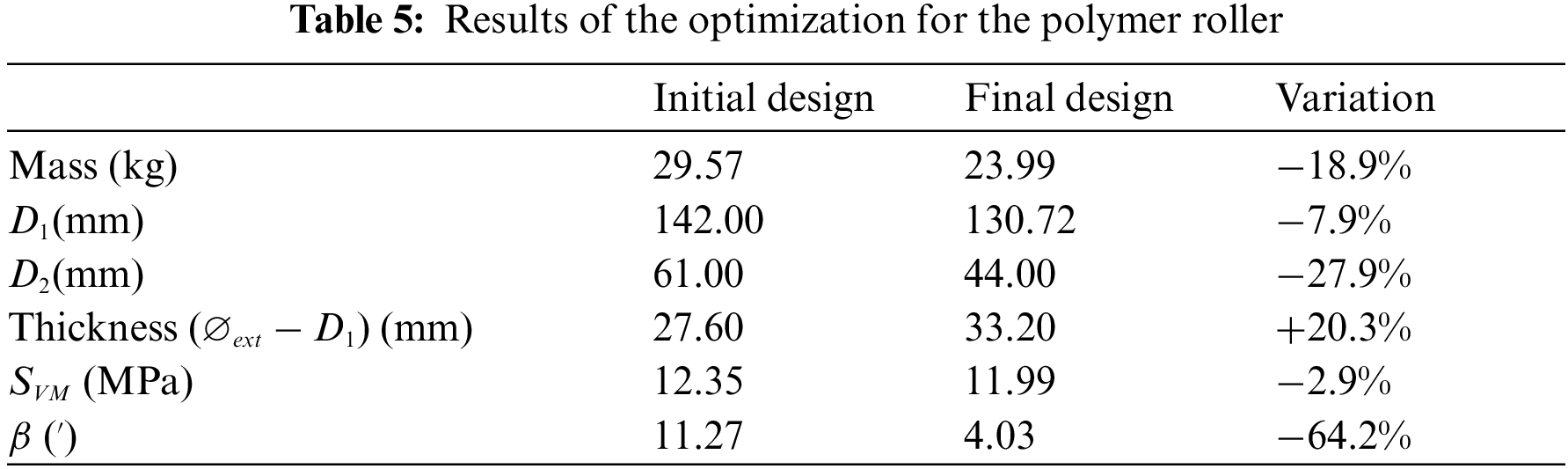
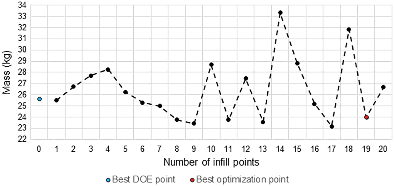
Figure 14: Evolution of the mass of the polymer roller during the optimization process

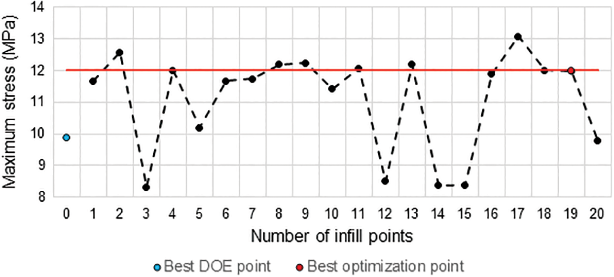
Figure 15: Evolution of the maximum von Mises stress during the optimization process (polymer roller)

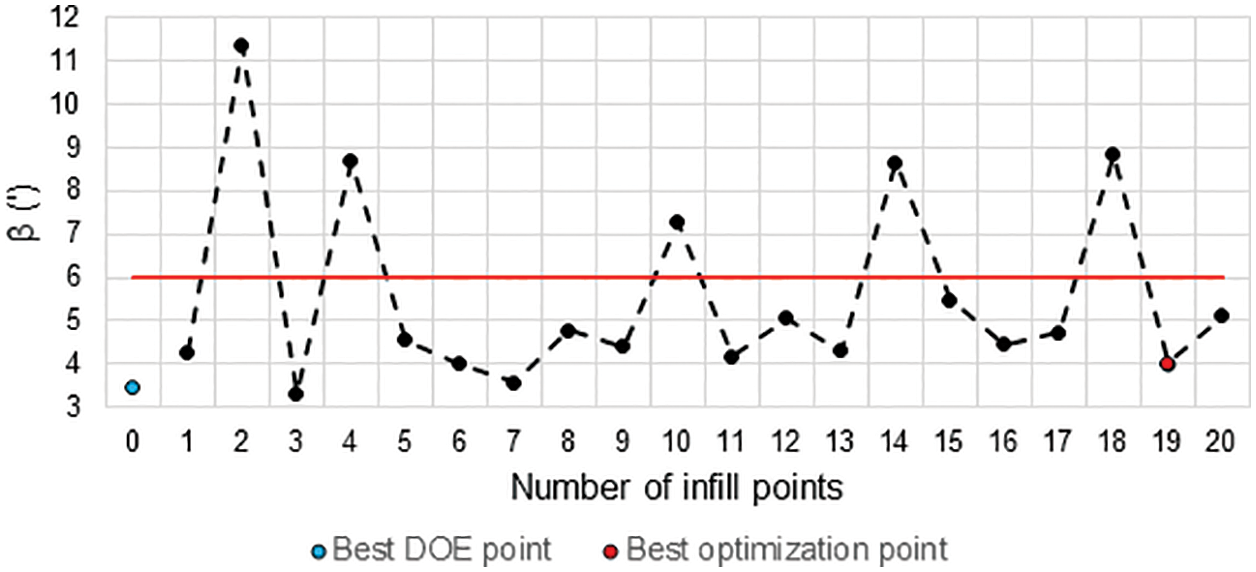
Figure 16: 16 Evolution of the bearing misalignment angle during the optimization process (polymer roller)

4  Concluding Remarks

The main objective of this work was to develop and apply a structural optimization methodology to minimize the mass of two different ore conveyor belt rollers. As the simulations of the finite element models of the rollers are time-consuming, a surrogate-based optimization strategy was used to alleviate the computational burden of the optimization process.

The first roller analyzed can be considered, from a structural point of view, to be made only of metal. In the second roller, the external component of the system (the external tube), which is in contact with the belt, as well as the components fixed to the bearings, are made of polymeric material. The designs are constrained by limits on the maximum stress and bearing misalignment angle.

For the metal roller, the functionality of the methodology when a penalty function is used was confirmed by optimizing two test cases in addition to the standard optimization case. For this roller design, a 32.3% reduction in relation to the initial mass was achieved with safety factors of 1.44 and 1.75 for the maximum stress and bearing misalignment angle, respectively. For the polymer roller, there was an 18.9% reduction in mass compared with the initial design with safety factors of 1.50 and 2.23 for the maximum stress and misalignment angle constraints. The reference values used for this roller were 18 MPa and 9', respectively.

The finite element simulations, which the results are employed to build the surrogate models, were carried out with some simplifications, e.g., the effects of the rotation of the roller, the effects of possible vibrations and the viscoelastic effect of the polymer were not taken into account. However, the analyses considered the recommendations in the current standard for the design of this type of mechanical system, and descriptions of simulations carried out using a comparable approach can be found in the literature.

Acknowledgement: The authors would like to thank Vale S.A. Company and the Institute of Technology Vale (ITV) for financing this research through the Project No. SAP 4600048682. The Brazilian funding agencies CAPES and CNPq are also acknowledged.

Funding Statement: This work was partially financed by Vale S.A. Company (https://www.vale.com) and the Institute of Technology Vale (ITV-https://www.itv.org) through the Project No. SAP 4600048682.

Conflicts of Interest: The authors declare that they have no conflicts of interest to report regarding the present study.

References

 1.  Ingale, P. B., Kadam, H. P., Narkar, K. M., Nighot, N. M. (2016). Design, analysis and weight reduction of roller of conveyor system through optimization. International Research Journal of Engineering and Technology, 3(6), 2329–2333. [Google Scholar]

 2.  Vasić, M., Stojanović, B., Blagojević, M. (2020). Failure analysis of idler roller bearings in belt conveyors. Engineering Failure Analysis, 117, 104898. DOI 10.1016/j.engfailanal.2020.104898. [Google Scholar] [CrossRef]

 3.  Zhao, L., Lin, Y. (2011). Typical failure analysis and processing of belt conveyor. Procedia Engineering, 26, 942–946. DOI 10.1016/j.proeng.2011.11.2260. [Google Scholar] [CrossRef]

 4.  ABNT (2017). Continuous conveyors-belt conveyors-rollers-design, selection and standardization, machines and mechanical equipment. ABNT NBR 6678: 2017 Standard (in Portuguese). [Google Scholar]

 5.  Christensen, P. W., Klarbring, A. (2008). An introduction to structural optimization. Linköping, Sweden: Springer Science & Business Media. [Google Scholar]

 6.  Arora, J. S. (2012). Introduction to optimum design. 3rd edition. San Diego: Academic Press. [Google Scholar]

 7.  Jiang, P., Zhou, Q., Shao, X. (2020). Surrogate model-based engineering design and optimization. Singapore: Springer. [Google Scholar]

 8.  Rodrigues, M. T., Luersen, M. A. (2020). Crashworthiness optimization of honeycomb structures under out of plane impact using radial basis functions. Materialwissenschaft und Werkstofftechnik, 51(5), 654–664. DOI 10.1002/mawe.201900233. [Google Scholar] [CrossRef]

 9.  Luersen, M. A., Le Riche, R. (2004). Globalized Nelder-Mead method for engineering optimization. Computers and Structures, 82(23–26), 2251–2260. DOI 10.1016/j.compstruc.2004.03.072. [Google Scholar] [CrossRef]

10. Peacock, A. (2000). Handbook of polyethylene: Structures: Properties, and applications. Boca Raton, USA: CRC Press. [Google Scholar]

11. Cheng, J. J., Polak, M. A., Penlidis, A. (2011). An alternative approach to estimating parameters in creep models of high-density polyethylene. Polymer Engineering & Science, 51(7), 1227–1235. DOI 10.1002/pen.21838. [Google Scholar] [CrossRef]

12. Zhao, B., Zhang, S., Sun, C., Guo, J., Yu, Y. X. et al. (2018). Aging behaviour and properties evaluation of high-density polyethylene (HDPE) in heating-oxygen environment. IOP Conference Series: Materials Science and Engineering, 369(1), 12021. DOI 10.1088/1757-899X/369/1/012021. [Google Scholar] [CrossRef]

13. Guermazi, N., Elleuch, K., Ayedi, H. F. (2009). The effect of time and aging temperature on structural and mechanical properties of pipeline coating. Materials & Design, 30(6), 2006–2010. DOI 10.1016/j.matdes.2008.09.003. [Google Scholar] [CrossRef]

14. Carrasco, F., Pages, P., Pascual, S., Colom, X. (2001). Artificial aging of high-density polyethylene by ultraviolet irradiation. European Polymer Journal, 37(7), 1457–1464. DOI 10.1016/S0014-3057(00)00251-2. [Google Scholar] [CrossRef]

15. Hutton, D. V. (2003). Fundamentals of finite element analysis. New York, USA: McGraw-Hill. [Google Scholar]

16. Berto, F., Campagnolo, A., Chebat, F., Cincera, M., Santini, M. (2016). Fatigue strength of steel rollers with failure occurring at the weld root based on the local strain energy values: Modelling and fatigue assessment. International Journal of Fatigue, 82, 643–657. DOI 10.1016/j.ijfatigue.2015.09.023. [Google Scholar] [CrossRef]

17. Johnson, K. L. (1985). Contact mechanics. 1st edition. Cambridge, UK: Cambridge University Press. [Google Scholar]

18. Gargiulo, E. P. (1980). A simple way to estimate bearing stiffness. Machine Design, 52(17), 107–110. [Google Scholar]

19. Wetter, M., Wright, J. (2004). A comparison of deterministic and probabilistic optimization algorithms for nonsmooth simulation-based optimization. Building and Environment, 39(8), 989–999. DOI 10.1016/j.buildenv.2004.01.022. [Google Scholar] [CrossRef]

20. Rao, S. S. (2009). Engineering optimization: Theory and practice. 2nd edition. New Jersey, USA: John Wiley & Sons. [Google Scholar]

21. Nelder, J. A., Mead, R. (1965). A simplex method for function minimization. The Computer Journal, 7(4), 308–313. DOI 10.1093/comjnl/7.4.308. [Google Scholar] [CrossRef]

22. Jin, R., Chen, W., Simpson, T. W. (2001). Comparative studies of metamodelling techniques under multiple modelling criteria. Structural and Multidisciplinary Optimization, 23(1), 1–13. DOI 10.1007/s00158-001-0160-4. [Google Scholar] [CrossRef]

23. Hussain, M. F., Barton, R. R., Joshi, S. B. (2002). Metamodeling: Radial basis functions, versus polynomials. European Journal of Operational Research, 138(1), 142–154. DOI 10.1016/S0377-2217(01)00076-5. [Google Scholar] [CrossRef]

24. Diaz Gautier, N. J., Silva, E. R., Manzanares-Filho, N., Ramírez Camacho, R. G. (2021). Automatic update of Gaussian and multiquadric shape parameter for sequential metamodels based optimization. Optimization and Engineering, 6(2), 639. DOI 10.1007/s11081-021-09692-2. [Google Scholar] [CrossRef]

25. Forrester, A. I. J., Sobester, A., Keane, A. J. (2008). Engineering design via surrogate modelling: A practical guide. Pondicherry, India: John Wiley & Sons. [Google Scholar]

26. Messac, A. (2015). Optimization in practice with MATLAB: For engineering students and professionals. UK: Cambridge University Press. [Google Scholar]

27. Park, G. J. (2007). Analytic methods for design practice. UK: Springer-Verlag London Limited. [Google Scholar]

28. Mack, Y., Goel, T., Shyy, W., Haftka, R. (2007). Surrogate model-based optimization framework: A case study in aerospace design. Evolutionary Computation in Dynamic and Uncertain Environments, pp. 323–342. Berlin, Heidelberg, Springer. [Google Scholar]

29. Parr, J. M., Keane, A. J., Forrester, A. I. J., Holden, C. M. E. (2012). Infill sampling criteria for surrogate-based optimization with constraint handling. Engineering Optimization, 44(1), 1147–1166. DOI 10.1080/0305215X.2011.637556. [Google Scholar] [CrossRef]

30. Bhosekar, A., Ierapetritou, M. (2018). Advances in surrogate based modeling, feasibility analysis, and optimization: A review. Computers & Chemical Engineering, 108(6), 250–267. DOI 10.1016/j.compchemeng.2017.09.017. [Google Scholar] [CrossRef]

31. Ye, P. (2019). A review on surrogate-based global optimization methods for computationally expensive functions. Software Engineering, 7(4), 68–84. DOI 10.11648/j.se.20190704.11. [Google Scholar] [CrossRef]

32. Smith, A. E., Coit, D. W. (1997). Constraint handling techniques-Penalty functions. In: Bäck, T., Fogel, D. B., Michalewicz, Z. (Eds.Handbook of evolutionary computation. 1st edition. UK: Oxford University Press. [Google Scholar]

33. Gosain, A., Sachdeva, K. (2019). Handling constraints using penalty functions in materialized view selection. International Journal of Natural Computing Research, 8(2), 1–17. DOI 10.4018/IJNCR. [Google Scholar] [CrossRef]

34. Martins, J. R., Ning, A. (2021). Engineering design optimization. UK: Cambridge University Press. [Google Scholar]

35. Iuliano, E., Quagliarella, D. (2019). Application of surrogate-based optimization techniques to aerodynamic design cases. Advances in Evolutionary and Deterministic Methods for Design, Optimization and Control in Engineering and Sciences, 48, 65–93. DOI 10.1007/978-3-319-89988-6_5. [Google Scholar] [CrossRef]

This work is licensed under a Creative Commons Attribution 4.0 International License, which permits unrestricted use, distribution, and reproduction in any medium, provided the original work is properly cited.