Evaluations of Chris-Jerry Data Using Generalized Progressive Hybrid Strategy and Its Engineering Applications

1  Introduction

Numerous researchers have struggled to model lifespan data with a long tail. In recent decades of literature, the oldest common heavy-tailed distributions were exponential, Lindley, and Pareto. A new one-parameter lifetime distribution by mixing two popular distributions, namely, exponential and gamma distributions, called the Chris-Jerry (CJ(μ)) distribution, has been introduced by Onyekwere et al. [1]. They also presented its mathematical properties and pointed out that it provides a good fit over the other eleven lifetime distributions in the literature. A random variable of lifetime, say Y, is said to follow the CJ distribution, denoted by Y∼CJ(μ) with scale parameter μ>0, then its probability density function (PDF) and cumulative distribution function (CDF) are given by

f(y;μ)=μ2μ+2(1+μy2)e−μy, y>0,(1)

and

F(y;μ)=1−[1+μy(μy+2)μ+2]e−μy(2)

respectively; see Onyekwere et al. [1]. Also, the respective reliability function (RF) and hazard rate function (HRF) of Y at time t>0 are

R(t;μ)=[1+μt(μt+2)μ+2]e−μt, t>0,(3)

and

h(t;μ)=μ2(1+μt2)μt(μt+2)+μ+2.(4)

In Fig. 1, for specific values of μ, several shapes of Eqs. (1) and (4) are displayed. It represents that the CJ density shapes allow for unimodal, decreasing, or increasing, while the failure rate shapes allow for bathtub-shaped.

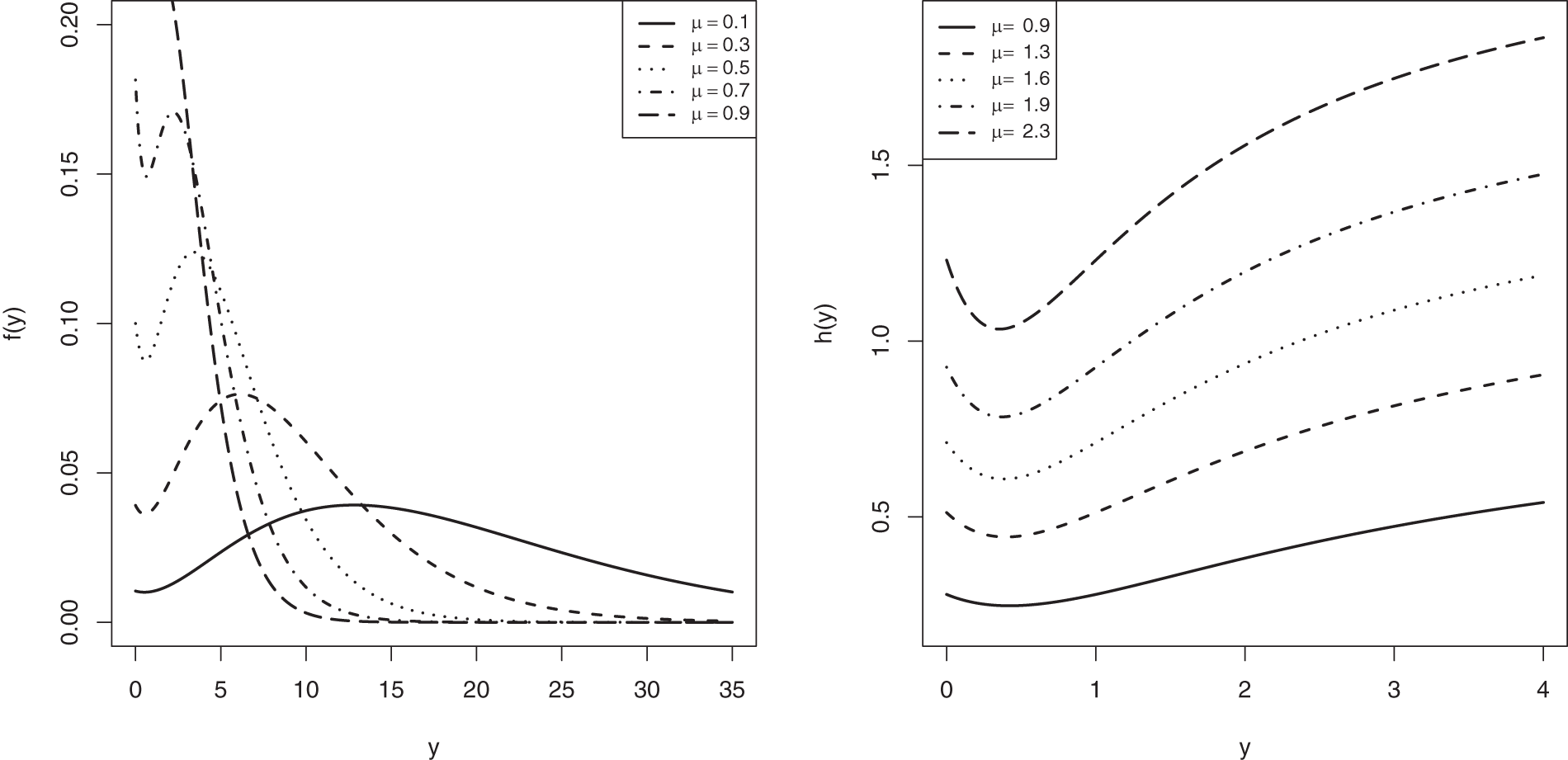
Figure 1: The CJ-PDF (left side) and CJ-HRF (right side) shapes

The reliability practitioner’s goal in life-testing research is to end the test before all of the tested subjects fail. It happens due to financial or time constraints. A hybrid censoring is a system that combines Type-I (time) and Type-II (failure) censoring techniques. One disadvantage of standard Type-I, Type-II, or hybrid censoring methods is that they do not allow units to be withdrawn from the test at locations other than the ultimate termination point; see Balakrishnan et al. [2]. Intermediate removal may be advantageous when a balance between decreased experimental duration and observation of at least some extreme lifespan is desired, or when some of the surviving units in the experiment that are removed early on can be re-purposed for future testing. These reasons and incentives direct dependability practitioners and theorists towards the field of progressive technique.

Progressive censoring Type-II (PC-T2) has been used the most, especially in reliability and survival analyses. It is preferable to the usual Type-II censoring approach. It can be advantageous in numerous scenarios, such as in professional environments and health-care settings. It enables the removal of operational experimental units throughout the experiment. Assume that m units fail out of n identical, where 1⩽m⩽n. Consider R=(R1,R2,…,Rm) to be fixed earlier than time. When the first failure occurs (say Y1:m:n), R1 (out of n−1) is eliminated from the examination. When the next failure Y2:m:n occurs, R2 (out of n−2−R1) is eliminated at random, and so on. When the mth failure happens, all remaining item(s) Rm are eliminated from the examination, then stop it; see Balakrishnan et al. [3].

If test subjects are very reliable, the PC-T2 has the disadvantage of having an extremely lengthy test time. To overcome this issue, Kundu et al. [4] proposed an alternate kind of censoring termed progressive hybrid censoring Type-I (PHC-T1), in which the examination terminates at T∙=min{T,Ym:m:n}, where T is a set period. When few failures are recorded before time T, the PHC-T1 has the disadvantage of not being usable. As a consequence, it may be impossible or exceedingly challenging to assess the parameters. Cho et al. [5] proposed a new generalized-progressive hybrid censoring (G-PHC) technique as a modification of the PHC-T1 by allowing us to see a specific number of failed units. As a result, it aims to minimize both overall testing time and unit failure costs. In the next section, this strategy will be described in more detail.

This research is novel as, for the first time, it compares two different methods of determining the CJ distribution for life parameters under imperfect information. Hence, we aim to complete the current work for the following motives:

•   The CJ model outperforms various competitor models in the literature, including the exponential, Lindley, and Muth lifespan models, in fitting engineering data sets, as proved later in the actual data section.

•   The estimations of the CJ distribution parameters of life under incomplete sampling plans have not been investigated yet in the literature. So, we consider the G-PHC strategy.

•   The proposed G-PHC plan is beneficial because it allows for the flexibility of stopping trials at a predefined period and reducing overall test length while keeping the desired features of a progressive system in practice. So, more accurate statistical estimates can be directly deduced from this study.

•   The CJ failure rate has a bathtub shape, which is a preferred occurrence in many practical areas.

As far as we understand, no discussion of inferential elements of the CJ distribution exists. Therefore, the purpose of this work, which employs the G-PHC strategy, has the next six objectives:

1.    Explore several estimation challenges of the CJ’s parameter (including: μ, R(t), and h(t)), in the presence of generalized progressively hybrid censored data, using maximum likelihood and Bayes estimation methodologies.

2.    Employ an approximation method called Monte-Carlo Markov-chain (MCMC) to evaluate the Bayesian estimations of the CJ parameters using a gamma conjugate prior and the squared error loss.

3.    Create the approximate confidence interval (ACI) as well as the highest posterior density (HPD) interval estimates for each unknown quantity.

4.    Install ‘maxLik’ (by Henningsen et al. [6]) and ‘coda’ (by Plummer et al. [7]) packages in R 4.2.2 programming environment to calculate the theoretical results of μ, R(t), and h(t) which cannot be represented in closed expressions.

5.    Assess the effectiveness of all acquired estimators via a series of numerical evaluations.

6.    Examine two engineering applications, based on repairable mechanical equipment and ball bearings data sets, to demonstrate the CJ distribution’s capacity to fit varied data types and adapt the offered methodologies to actual practical circumstances.

The next parts are organized as follows: Section 2 describes the proposed G-PHC plan. Maximum likelihood and Bayes’ estimations are provided in Sections 3 and 4, respectively. Simulation findings are presented in Section 5. Two engineering applications are examined in Section 6. Finally, several conclusions, remarks, and recommendations are listed in Section 7.

2  G-PHC Plan

This section explains the G-PHC procedure. Let us give {Y1,Y2,…,Yn} to the lives produced by a distribution with CDF F(y;μ) and PDF f(y;μ). Let T>0 be a fixed time (where T∈(0,∞)) and r<m⩽n be pre-fixed integers with a fixed plan R (where m+∑imRi=n). When Y1:m:n recorded, R1 of n−1 is destroyed randomly. Similarly, when Y2:m:n recorded, R2 of n−2−R1 is removed, and so on. End the examination at T∙=max{Yr:m:n,min{Ym:m:n,T}}. If T<Yr:m:n<Ym:m:n (say, Case-1), the examination is ended at Yr:m:n; if Yr:m:n<T<Ym:m:n (say, Case-2), the examination is ended at T where j is the number of failed units recorded up to T; otherwise, when Yr:m:n<Ym:m:n<T (say, Case-3), the examination is ended at Ym:m:n. However, let {Y,R} be a G-PHC sample from a continuous population. Then, the joint PDF (say ℒξ(⋅)) is

ℒξ(μ|Y)=Aξ[R(T;μ)]R∗∏i=1Dξf(yi:m:n;μ)[R(yi:m:n;μ)]Ri, ξ=1,2,3,(5)

where RD1=n−r−∑i=1r−1Ri and RD3=n−m−∑i=1m−1Ri. The main benefit that would be acquired by an investigator when dealing with G-PHC is that it enables us to obtain r failures, although the investigator would prefer to record m failures. In Table 1, the G-PHC notations are presented.

Recently, several researchers have done G-PHC-based investigations; for example, Koley et al. [8], Elshahhat [9], Wang [10], Lee et al. [11], Lee [12], Zhu [13], Singh et al. [14], Elshahhat et al. [15], Maswadah [16], later, Alotaibi et al. [17].

We have two limitations in this study, as follows: (i) All inferential methodologies discussed in the next sections are investigated based on the assumption that the quantity j at T is higher than or equal to 1; (ii) All CJ parameters μ, R(t), and h(t) are always assumed to be unknown.

3  Likelihood Inference

Using (1), (2) and (5), we can express Eq. (5), where yi=yi:m:n for simplicity, as

ℒξ(μ|y)∝μ2Dξe−μψ(μ+2)n∏i=1Dξ(1+μyi2)[φ(yi;μ)]Ri[φ(T;μ)]R∗,(6)

where y¯=Dξ−1∑i=1Dξyi, ψ=TR∗+Dξy¯+∑i=1DξyiRi, φ(yi;μ)=μyi(μyi+2)+μ+2, and φ(T;μ)=μT(μT+2)+μ+2. The natural logarithm of (6) becomes

ℓξ(μ|y)∝−nlog⁡(μ+2)+2Dξlog⁡(μ)−μψ+∑i=1Dξlog⁡(1+μyi2)+∑i=1DξRilog⁡[φ(yi;μ)]+R∗log⁡[φ(T;μ)].(7)

As a result, the maximum likelihood estimator (MLE), denoted by μ^, of μ, can be offered by directly maximizing (7) with the following nonlinear normal equation:

2Dξμ^−1−ψ−nμ^+2+∑i=1Dξyi21+μ^yi2+∑i=1DξRiφ∙(yi;μ^)φ(yi;μ^)+R∗φ∙(T;μ^)φ(T;μ^)=0,(8)

where φ∙(yi;μ^)=2yi(μ^yi+1)+1, and φ∙(T;μ^)=2T(μ^T+1)+1.

Obviously, from (8), the MLE μ^ of μ cannot be derived in a closed expression. Clearly, depending on the structure of the likelihood function (5), the target MLE μ^ cannot be represented in a closed solution. This complexity will depend on iterative numerical methods to calculate the MLE when there is no analytical solution to the likelihood equation.

It is essential to investigate the existence and uniqueness of the MLE μ^. The complex form in (8) makes it difficult to verify these features theoretically. To address this issue, we simulate a G-PHC sample from CJ (0.5) with (n,m,T)=(50,25,2.5) and Ri=1, i=1,…,m. After that, we get the MLE for μ is 0.7361. Fig. 2 depicts the log-likelihood and normal-equation functions given by (7) and (8), respectively. It provides how the vertical line (which represents the MLE of μ) intersects the log-likelihood curve (at the apex) and the normal equation curve (at the zero point). As a result, the MLE μ^ of μ exists and is unique.

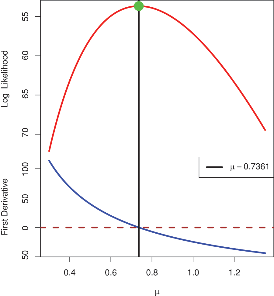
Figure 2: The log-likelihood and normal-equation curves

Once μ^ is found, by replacing μ with μ^, it is straightforward to estimate the RF (2) and HRF (4), respectively as:

R^(t)=[1+μ^t(μ^t+2)μ^^+2]e−μ^t

and

h^(t)=μ^2(1+μ^t2)μ^t(μ^t+2)+μ^+2.

Aside from the point estimate, the 100(1−γ)% ACI of μ, R(t), or h(t) is of importance. Using the asymptotic features of μ^, we acquire the ACIs for all unknown parameters. Because of the complexity of the Fisher information, creating V(⋅) matrix using the observed I(⋅)|μ=μ^ matrix is more convenient. As a result, the V(⋅) matrix may be estimated as:

V(μ^)=I−1(μ)|μ=μ^,=[−d2ℓdμ2]μ=μ^−1,(9)

where

d2ℓdμ2=−2Dξμ^2+n(μ^+2)2−∑i=1Dξyi4(1+μ^yi2)2+∑i=1DξRi{2yi2φ(yi;μ^)−[φ∙(yi;μ^)]2[φ(yi;μ^)]2}+R∗{2T2φ(T;μ^)−[φ∙(T;μ^)]2[φ(T;μ^)]2}.

Thus, the 100(1−γ)% ACI of μ at a significance level γ% is given by

μ^∓zγ2V(μ^),

where zγ2 is the upper (γ2)th standard-normal percentile point.

Additionally, to build the 100(1−γ)% ACIs of R(t) and h(t), we must first obtain the variances of their estimators R^(t) and h^(t). Following Greene [18], the respective variances of h^(t) and h^(t), denoted by V^R and V^h, are obtained as

V^R=ℋRV(μ^)ℋR⊤|μ=μ^andV^h=ℋhV(μ^)ℋh⊤|μ=μ^,

where φ(t;μ)=μt(μt+2)+μ+2, φ∙(t;μ)=2t(μt+1)+1,

ℋR=te−μt[(μ+2)−1(2+μ{2t−((μ+2)−1+t)(2+μt)})−1]

and

ℋh=μ(3μt2+2)φ(t;μ)−μ2(1+μt2)φ∙(t;μ)[φ(t;μ)]2.

As a consequence, 100(1−γ)% ACIs of R(t) and h(t) can be acquired respectively as

R^(t)∓zγ2V^Randh^(t)∓zγ2V^h.

4  Bayesian Inference

Bayesian setup is an effective method for integrating knowledge in challenging scenarios. Briefly, we report some of its advantages and inconveniences as follows:

•   Some advantages of employing Bayesian analysis:

–   It offers a natural and logical approach to combining previous knowledge with data inside a strong theoretical framework for decision-making.

–   It gives conditional and accurate conclusions without the need for asymptotic approximations.

–   It gives interpretable responses and follows the probability principle.

–   It offers a suitable environment for a variety of models, including hierarchical models and missing data issues.

•   Some inconveniences of employing Bayesian analysis:

–   It does not explain how to choose a previous. There is no proper way to select a predecessor.

–   It can produce posterior distributions that are heavily influenced by the priors.

–   It often comes with a high computational cost, especially in models with a large number of parameters.

–   It provides simulations that produce slightly different answers unless the same random seed is used.

However, the major topic of discussion in this part is the Bayesian inference of μ, R(t), and h(t). Prior distributions and loss functions, it should be noted, both play critical roles in Bayes’ paradigm. This paper considers the squared-error loss as the most useful symmetric loss in the literature. Without loss of generality, other loss functions such as Linex, entropy, or others can be easily incorporated.

Choosing a prior for an unknown parameter might be difficult. In reality, as stated by Arnold et al. [19], there is no accepted method for picking an appropriate prior for Bayesian estimation. Because the CJ parameter μ has values between 0 and ∞, the gamma distribution is a suitable prior choice to adapt μ. Assume that μ∼Gamma(a,b), then its PDF (say ω) becomes

ω(μ;a,b)∝μa−1e−bμ, a,b>0.(10)

From (6) and (10), the posterior PDF (say Ω) of μ is

Ωξ(μ|{y})=C−1μ2Dξ+a−1e−μ(b+ψ)(μ+2)n∏i=1Dξ(1+μyi2)[φ(yi;μ)]Ri[φ(T;μ)]R∗,(11)

where

C=∫0∞μ2Dξ+a−1e−μ(b+ψ)(μ+2)n∏i=1Dξ(1+μyi2)[φ(yi;μ)]Ri[φ(T;μ)]R∗dμ.

Using (11), due to the nonlinear form in (6), the Bayes estimate of μ, R(t), or h(t) is difficult to acquire analytically. As a result, using the MCMC methodology, we produce Markovian samples from (11), and then we acquire the Bayes estimate and create the appropriate HPD interval for each unknown parameter. In this regard, for more details about the MCMC mechanism, we refer to Asadi et al. [20] and Nagy et al. [21]. However, Fig. 3 demonstrates that the posterior PDF (11) is identical to the normal density. So, in the next steps, we must apply the Metropolis-Hastings (MH) approach to produce the Bayes estimates and build the HPD intervals for all unknown subjects:

Step 1. Set μ(0)=μ^ (initial value).

Step 2. Put ϖ=1.

Step 3. Generate μ⋆ using N(μ(ϖ−1),V^(μ^)).

Step 4. Obtain M=min[1,Ωξ(μ⋆|{y})Ωξ(μ(ϖ−1)|{y})].

Step 5. Obtain a variate u from U(0,1).

Step 6. If u⩽M, set μ(ϖ)=μ⋆, else, set μ(ϖ)=μ(ϖ−1).

Step 7. Redefine R(t) and h(t) via μ replacing by μ(ϖ) in (3) and (4), respectively.

Step 8. Set ϖ=ϖ+1.

Step 9. Redo Steps 3–8 B times, then ignore the first samples (say B∘) burn-in period to acquire B samples of μ, R(t), or h(t) (say κ) as [κ(B∘+1),κ(B∘+2),…,κ(B)].

Step 10. Find κ~ as

κ~=1B∙∑ϖ=B∘+1Bκ(ϖ),

where B∙=B−B∘.

Step 11: Compute the (1−γ)100% HPD interval of κ via sorting its simulated MCMC variates as κϖ for ϖ=B∘+1,…,B and conducting the technique by Chen et al. [22] as

(κ(ϖ∗),κ(j∗+(1−γ)B∙)),

where b∗ is specified as

κ(ϖ∗+[(1−γ)B∙])−κ(ϖ∗)=min1⩽ϖ⩽γB∙(κ(ϖ+[(1−γ)B∙])−κ(ϖ)).

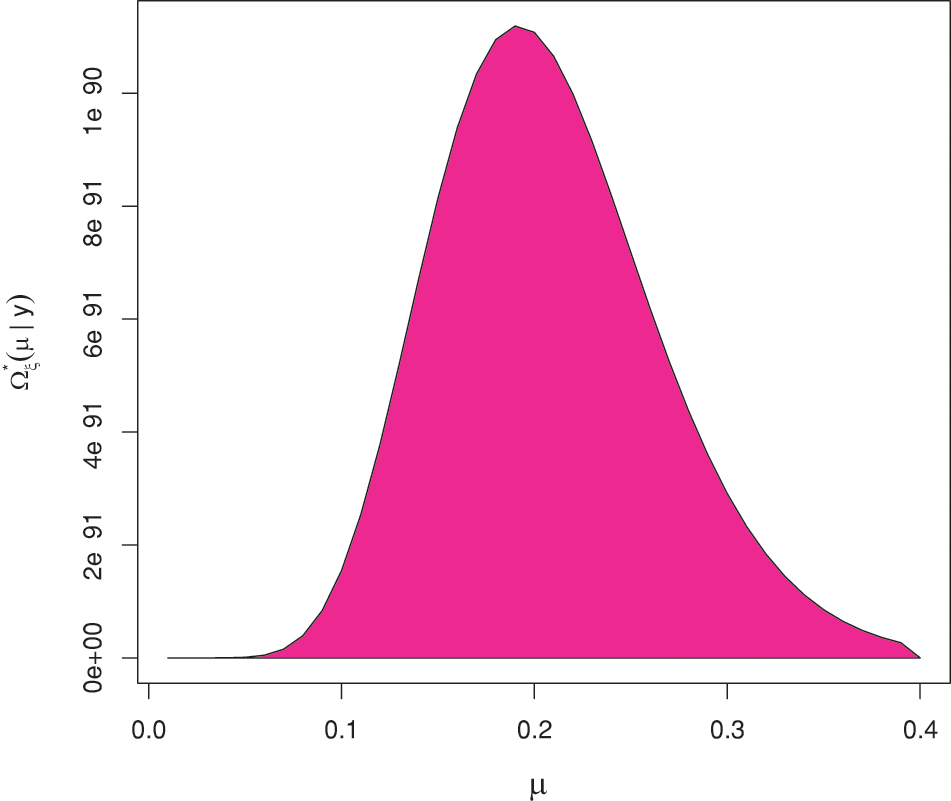
Figure 3: The posterior PDF of μ

5  Numerical Evaluations

In this part, to assess the accuracy and utility of the acquired estimates of μ, R(t), and h(t) presented in the preceding sections, we implement several Monte Carlo tests.

5.1 Simulation Design

First, to get the point (or interval) estimate of μ, R(t), or h(t), we repeat the G-PHC mechanism 1,000 times for each μ(=0.5,1.5). Taking t=0.5, the plausible value of (R(t), h(t)) is taken as (0.95403, 0.09184) and (0.75073, 0.55618) for μ=0.5 and 1.5, respectively. Assigning T(=2.5, 7.5), n(=40, 80), several failure probabilities (FPs%) of r and m are utilized, namely: FP[r]=rn(=25, 37.5)% and FP[m]=mn(=50, 75)%. Additionally, for each set of (n,m), different PC-T2 deigns R are also considered, namely:

Scheme-A:(n−m,0(m−1)),Scheme-B:(0(m2−1),n−m,0(m2)), and Scheme-C:(0(m−1),n−m),

where 0(m−1) means 0 is repeated m−1 times.

To get a G-PHC sample from CJ(μ), do the following generation steps:

Step 1. Assign the actual value of μ.

Step 2: Simulate an ordinary PC-T2 sample of size m as:

a.   Generate ω1,ω2,…,ωm independent observations from uniform U(0,1) distribution.

b.   Set gi=ωi(i+∑l=m−i+1mRl)−1, i=1,2,…,m.

c.   Set Ui=1−gmgm−1⋯gm−i+1 for i=1,2,…,m.

d.   Set Y(i)=F−1(ui;μ), i=1,2,…,m, PC-T2 order statistics from (2).

Step 3.Determine j at T.

Step 4. Specify the G-PHC data type as:

a.   {Y1,…,Yr} if T<Yr<Ym, it is Case-1;

b.   {Y1,…,Yj} if Yr<T<Ym, it is Case-2;

c.   {Y1,…,Ym} if Yr<Ym<T, it is Case-3.

As soon as the 1,000 G-PHC samples are collected, the offered frequentist point/interval estimates of μ, R(t), and h(t) are acquired via the ‘maxLik’ package. In Bayesian calculations, to highlight the performance of the suggested gamma density prior, for each given value of μ, two different sets of (a,b) are utilized, namely: (i) At μ=0.5: Prior-1:(2.5,5) and Prior-2:(5,10); and (ii) At μ=1.5: Prior-1:(7.5,5) and Prior-2:(15,10). Here, the values of (a,b) are specified such that the prior mean is translated to the genuine parameter value of μ.

Simulating 12,000 MCMC variates and then burning-in the first 2,000 draws, the Bayes MCMC and 95% HPD interval estimates of μ, R(t) and h(t) are calculated by the ‘coda’ package. Though MCMC is a strong tool in statistical programming for assessing complicated models and posterior distributions, it requires extensive inspection and tweaking to ensure its validity and efficiency. The trace (thinning) process, which involves picking different points from the sample at each preset step to form an independent sample, is considered for this objective. In Fig. 4, using Scheme-A, Prior-1, and (T,n,m,r)=(2.5,40,20,10), we plotted the trace diagrams of μ. It ensures that the MCMC draws are sufficiently mixed and that the posterior density draws of μ are strongly symmetric. It also supports the MH sampler for μ that has been proposed.

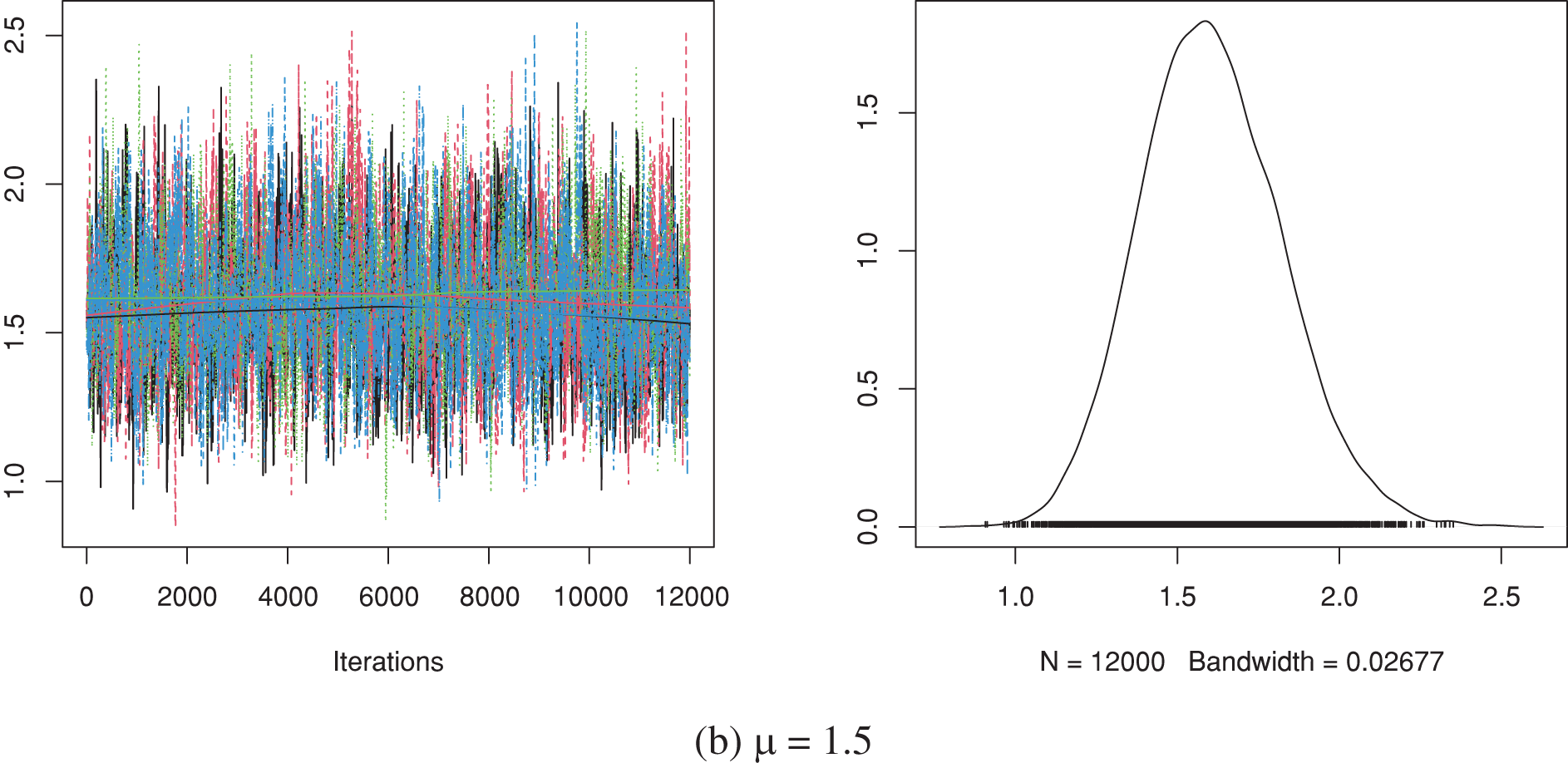
Figure 4: Trace (left) and density (right) diagrams of μ

Next, we calculate the following quantities of κ, R(t), or h(t) (say κ):

•   Average Point Estimate (Av.PE): Av.PE(κ¯)=11000∑i=11000κ¯(i),

•   Root Mean Squared Error (RMSE): RMSE(κ¯)=11000∑i=11000(κ¯(i)−κ)2,

•   Mean Relative Absolute Bias (MRAB): MRAB(κ¯)=11000∑i=110001κ|κ¯(i)−κ|,

•   Average Confidence Length (ACL): ACL(1−γ) (κ)=11000∑i=11000(𝒰κ¯(i)−ℒκ¯(i)),

•   Coverage Percentage (CP): CP(1−γ) (κ)=11000∑i=11000I(ℒκ¯(i);𝒰κ¯(i))(κ),

•   where κ¯(i) is the desired estimate of κ at i th sample, I(⋅) is indicator function, (ℒ(⋅),𝒰(⋅)) is two-sided of (1−γ)100% ACI (or HPD) of κ.

5.2 Simulation Results and Discussions

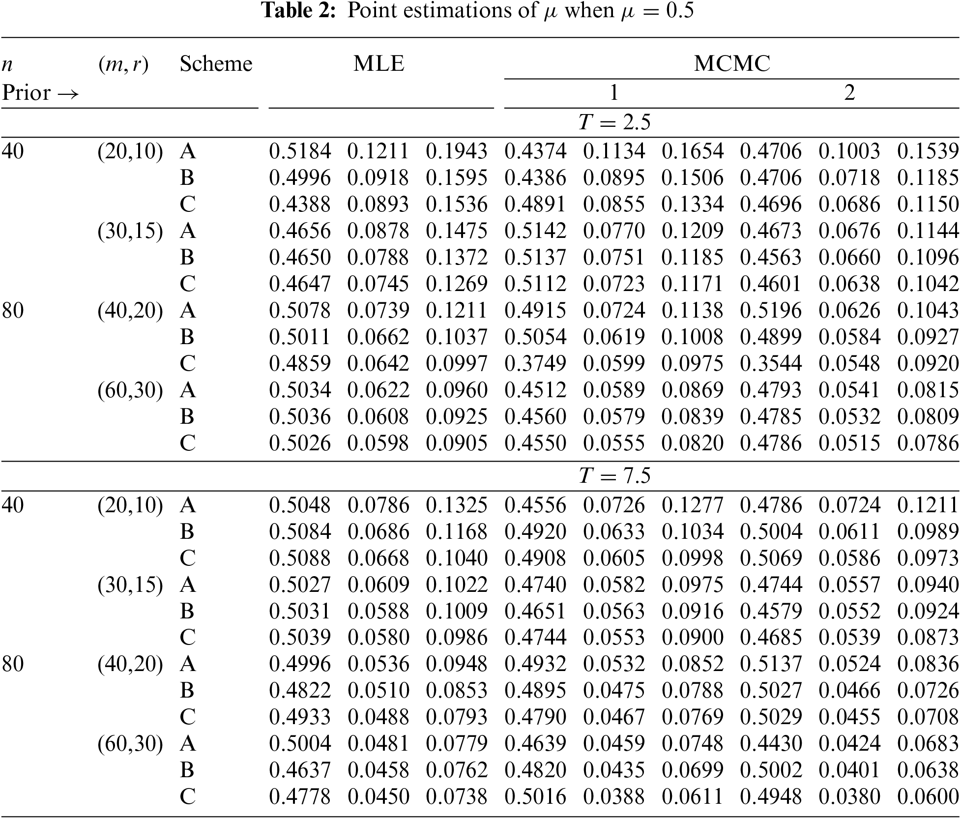
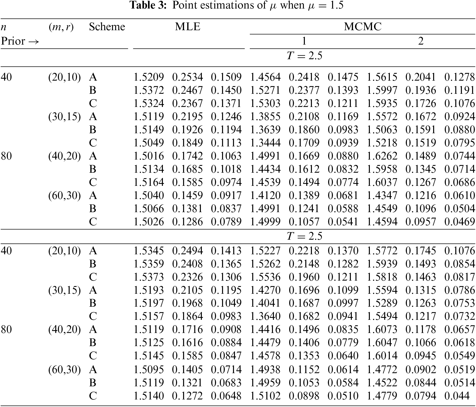
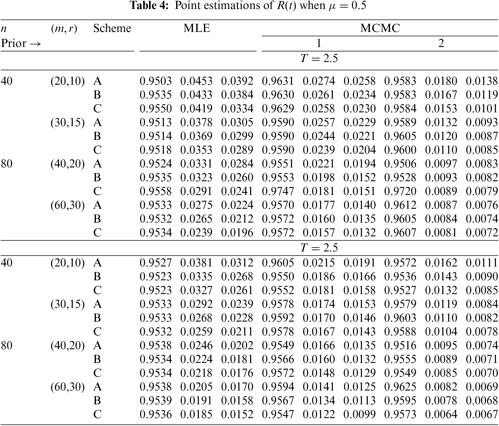
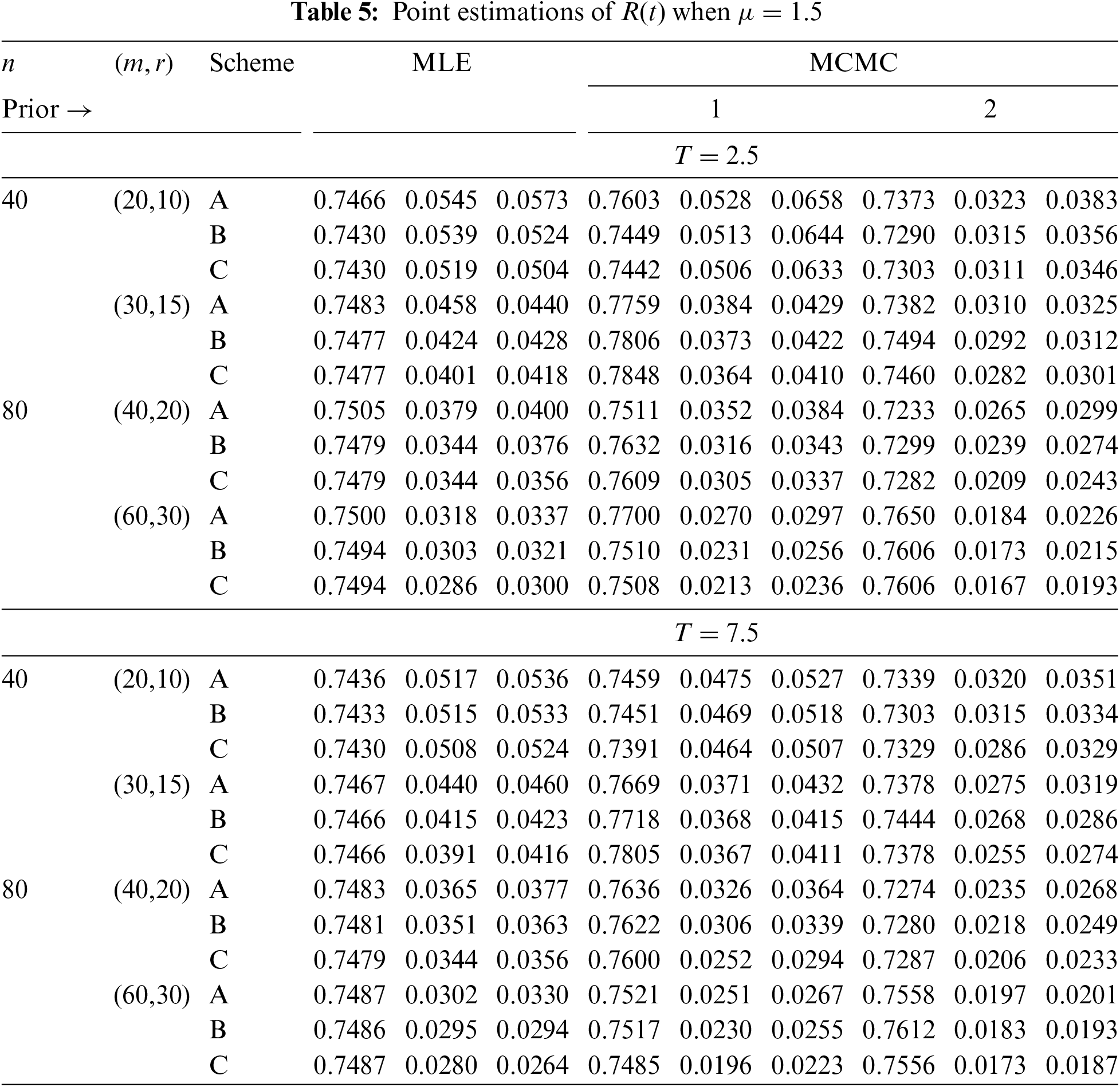
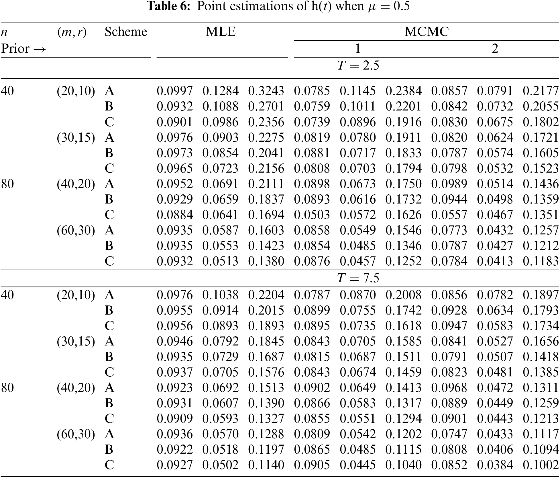
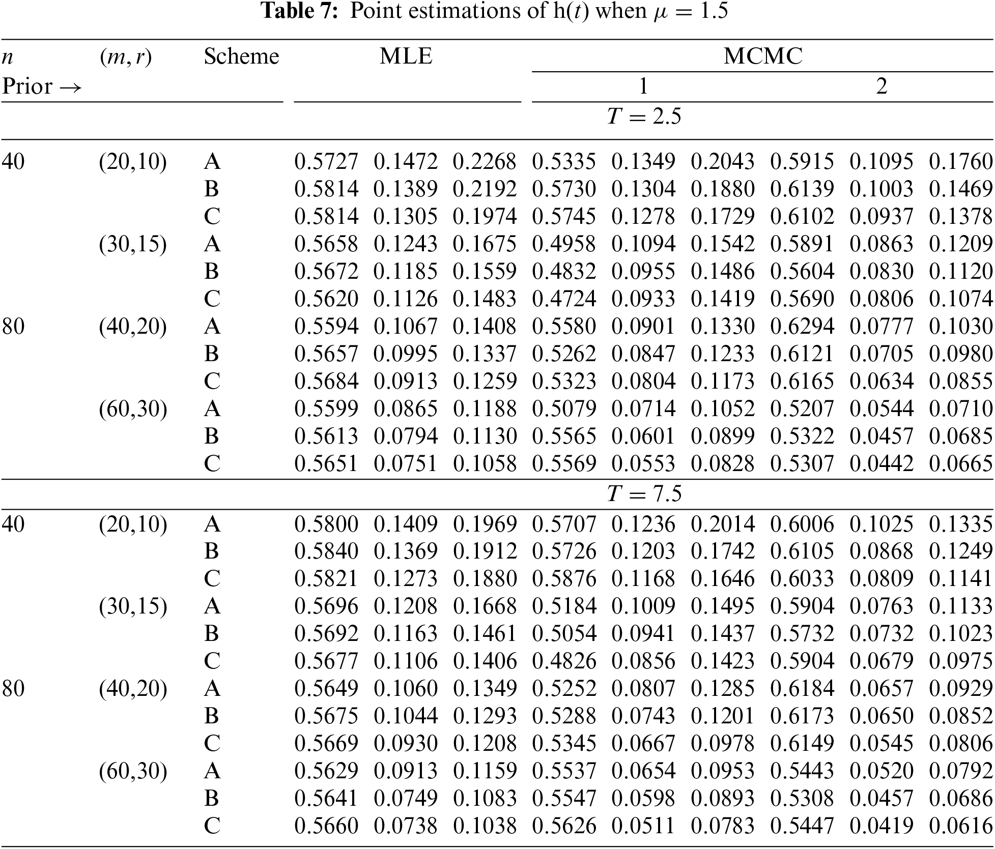
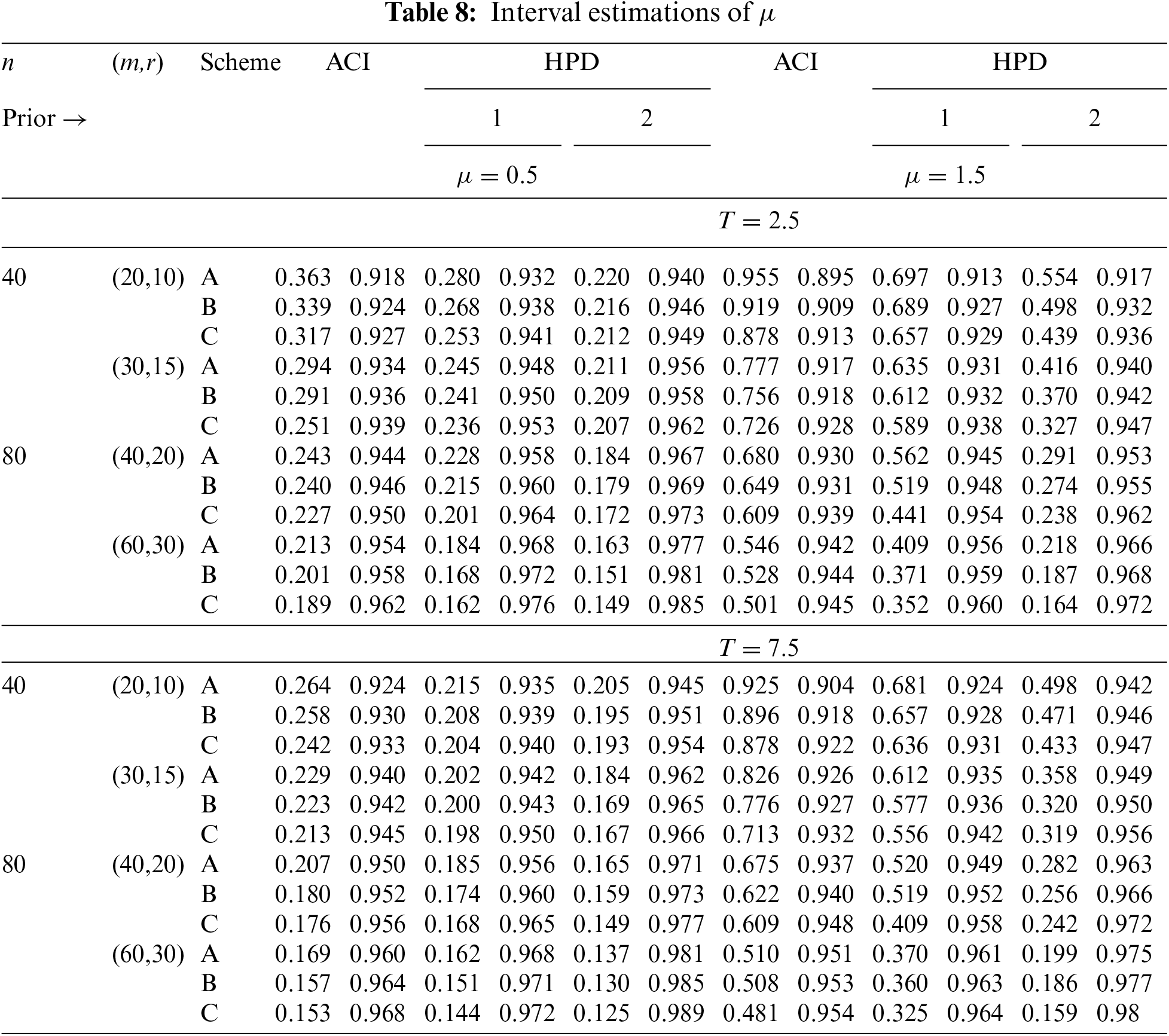
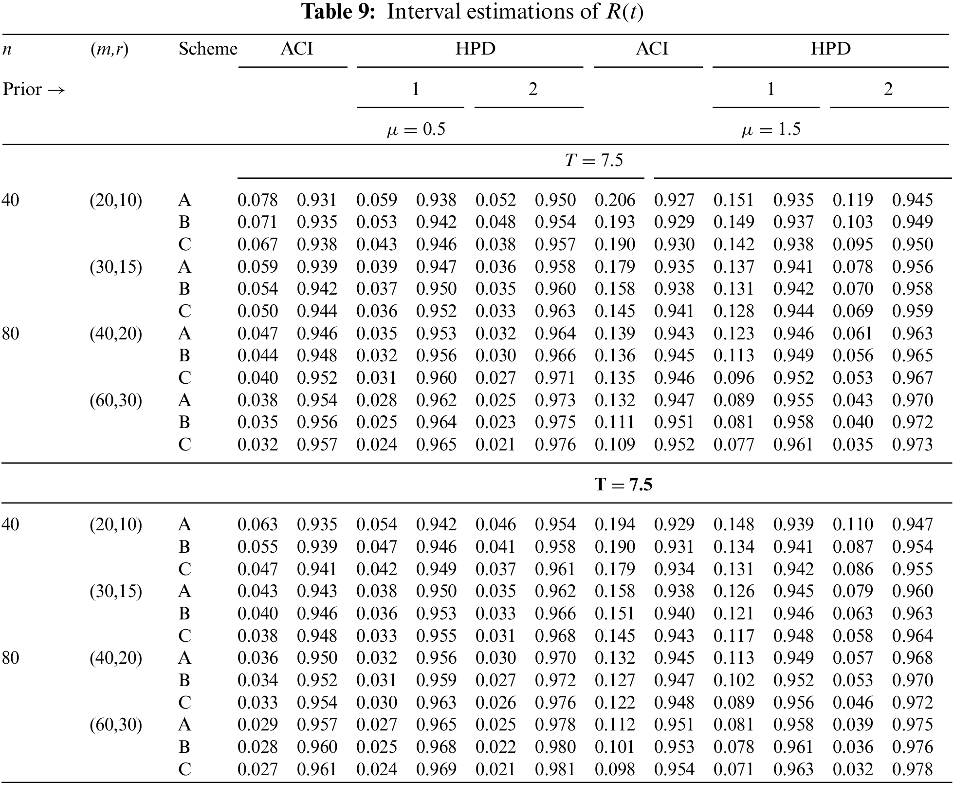
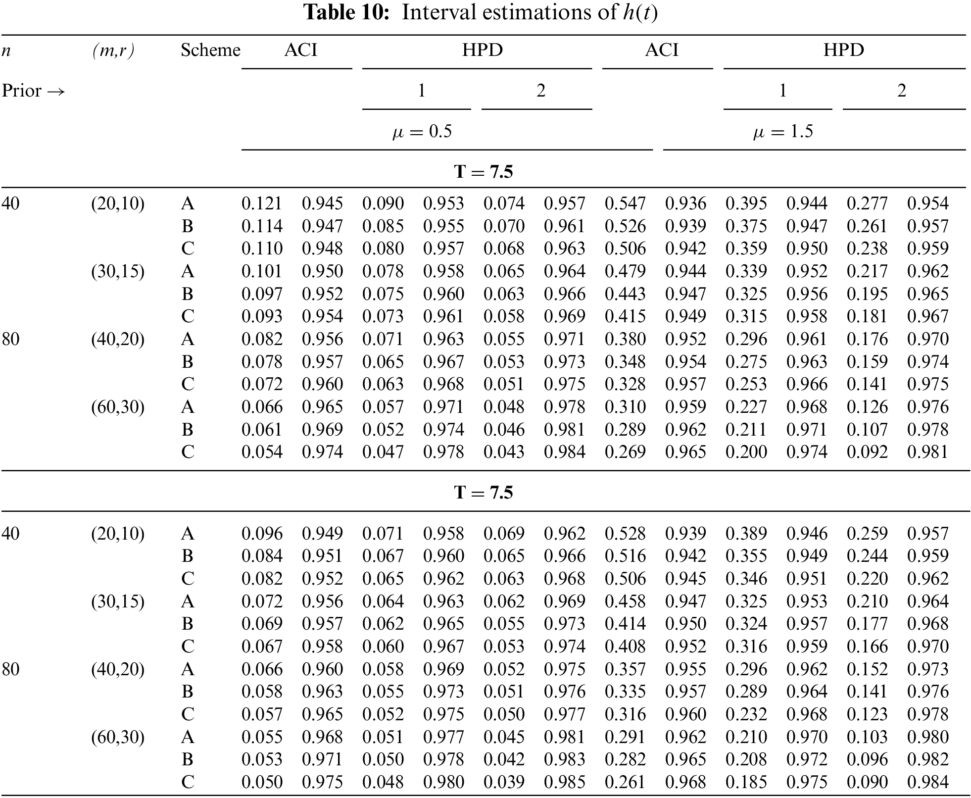
In Tables 2–7, the Av.PEs, RMSEs, and MRABs are reported in the first, second, and third columns, respectively, while in Tables 8–10, the ACLs and CPs are reported in the first and second columns, respectively. Obviously, an effective estimator of μ, R(t), or h(t) should correspond to the lowest level of RMSE, MRAB, and ACL as well as the highest level of CP. From Tables 2–10, we can list the following observations:

•   All acquired results of μ, R(t), or h(t) behaved well.

•   As n(or FP[r]% or FP[m]%) increases, all estimation findings of μ, R(t), and h(t) perform well. This note is also reached when ∑i=1mRi tends to decrease.

•   To acquire a highly efficient estimation of μ, R(t), or h(t), the practitioner must decrease the total progressive patterns or increase the size of at least one member of n, m, or r.

•   As T increases, for each value of μ, the acquired RMSE, MRAB, and ACL values of μ, R(t), or h(t) decrease while their CP values increase.

•   As T grows, for each value of μ, the accuracy for all estimates of all parameters becomes good.

•   As μ increases, the acquired RMSE, MRAB, and ACL values of μ, R(t), or h(t) increase.

•   As μ increases, the acquired CP values of μ, R(t), or h(t) decrease.

•   In most cases, the simulated CPs of μ, R(t), or h(t) are close to the pre-specified nominal 95% level.

•   Due to the availability of gamma prior information, Bayesian evaluations of μ, R(t), or h(t) perform satisfactorily when compared to conventional estimates.

•   For each value of μ, the Bayes’ method via Prior-2-based produces highly precise results over competitors. This observation is understandable given that the variance linked to Prior-2 is lower than the variance associated with Prior-1. In the case of HPD interval estimations, a similar result is obtained.

•   The HPD interval estimations of μ, R(t), or h(t) perform better in the presence of prior knowledge coming from Prior-2 than those gathered from Prior-1, while both behaved well compared to those developed from the asymptotic interval estimations.

•   Comparing the suggested PC-T2 designs A, B, and C, the offered point (or interval) findings using Scheme-C (or conventional Type-II censoring) of all parameters perform better than others.

•   To summarize, when the reliability practitioner performs the proposed strategy, it is advised to explore the Chris-Jerry lifetime model using Bayes’ MCMC technique via the Metropolis-Hastings sampler.

6  Engineering Applications

This part analyzes two sets of actual data from the engineering field to assess the effectiveness of the estimating methods in practice. In a similar way, without loss of generality, one can easily apply the same proposed methods to other actual datasets from scientific fields, e.g., medicine, physics, chemistry, etc.

6.1 Mechanical Equipment Data

To highlight the utility of methodologies proposed for an actual phenomenon, an engineering application representing the failure times for 30 items of repairable mechanical machines (RMM) is analyzed in this subsection; see Table 11. Nassar et al. [23] reanalyzed the RMM data set after it was first provided by Murthy et al. [24].

From the full RMM data, to check the effectiveness of the CJ model, we shall compare its fit to other five models in the literature, namely: XLindley (XL(μ)) by Chouia et al. [25], Xgamma (XG(μ)) by Sen et al. [26], Muth (M(μ)) discussed by Irshad et al. [27], Lindley (L(μ)) by Ghitany et al. [28], and exponential (E(μ)) reviewed by Tomy et al. [29]. To establish this objective, behind the Kolmogorov–Smirnov (KS) distance (with its p-value), we obtain the negative log–likelihood (NL), Akaike (A), consistent Akaike (CA), Bayesian (B), and Hannan–Quinn (HQ); see Table 12. The MLE (with its standard–error (St.Er)) is utilized to evaluate all proposed criteria.

It shows, from Table 12, that the CJ distribution has the best values of all proposed criteria than its competing distributions. So, based on the RMM data, depending on all considered criteria, we decided that the CJ lifespan model is superior to the others. Fig. 5 shows the fitted PDFs, the fitted RFs, and probability–probability (PP) for the CJ and its competing models. As expected, it confirms the numerical findings established in Table 12.

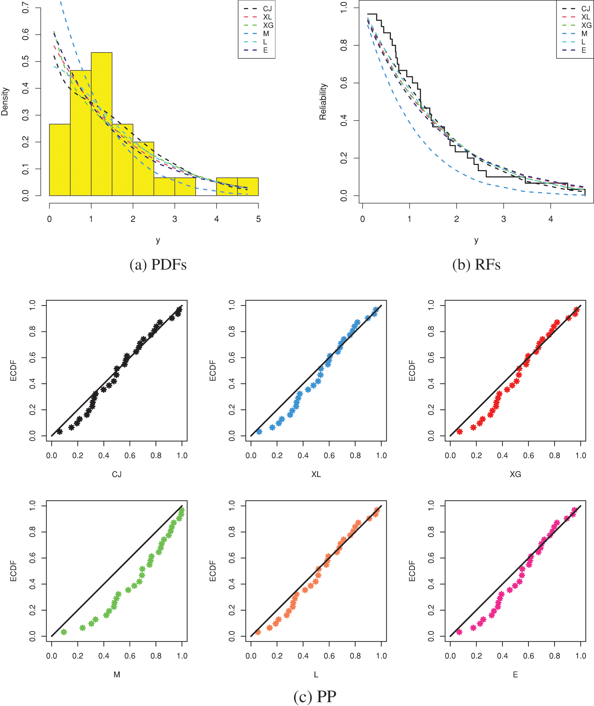
Figure 5: Fitting plots from RMM data

To examine the acquired theoretical estimators of μ, R(t) and h(t) from the RMM data set, by taking (m,r)=(15,10) based on different choices of R and T, three G-PHC samples are created; see Table 13. From Table 13, the point estimates (with their St.Ers) as well as the interval estimates (with their interval widths) of μ, R(t), and h(t) at t=0.75 are calculated; see Table 14. Because there is no additional information about the CJ(μ) parameter in the RMM data set, the Bayes estimates are generated by running the MCMC sampler 50,000 times and disregarding the first 10,000 times as burn-in. Table 14 reveals that the estimation outputs of all parameters are nearly identical.

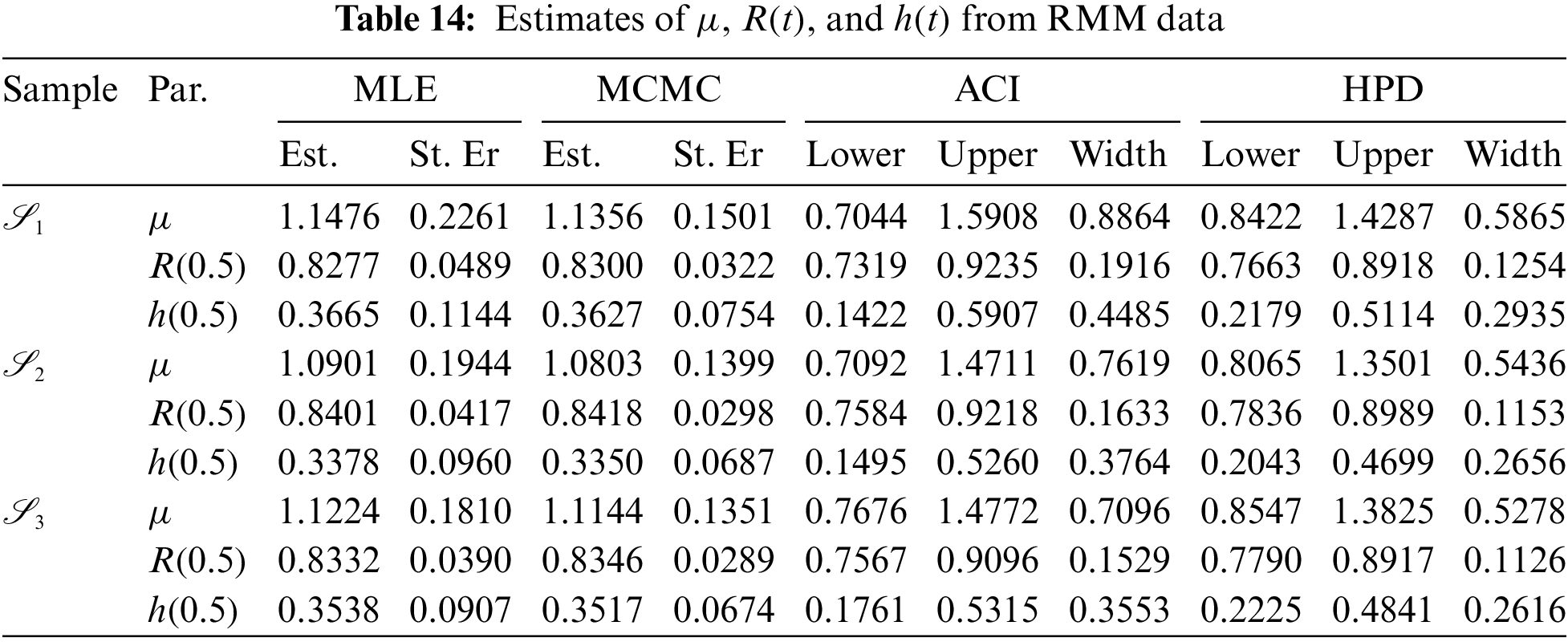
At varying options of μ, Fig. 6 stands that the acquired μ^ based on 𝒮i, for i=1,2,3 existed and is unique. We also suggest using the value of μ^ in each sample (in Table 14) as an initial guess for running the required Bayesian evaluations. Fig. 7, based on 𝒮1 (as an example), shows that the collected Markovian variates of μ, R(t), or h(t) are converged satisfactorily, as well as that those iterations are nearly symmetrical.

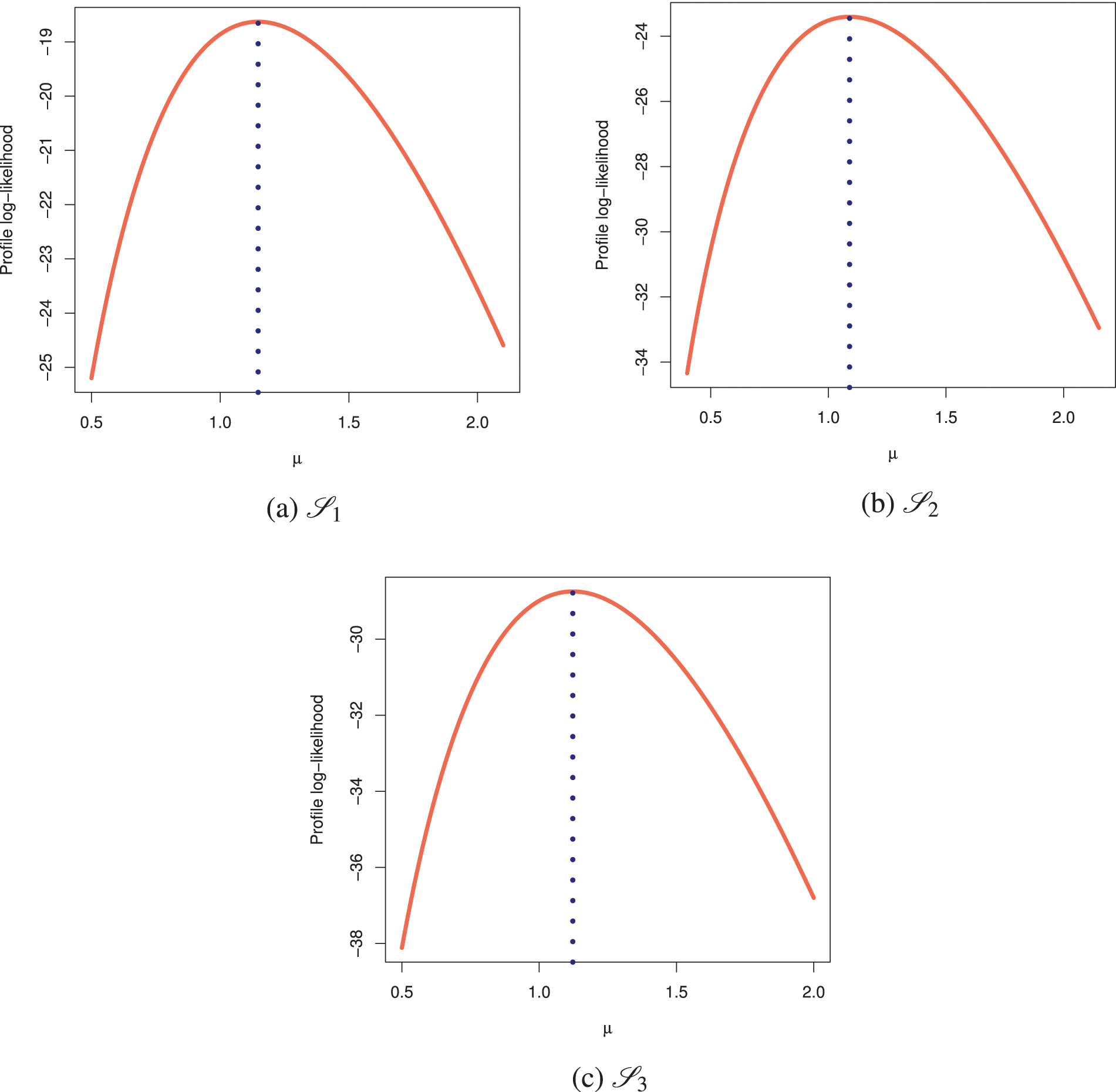
Figure 6: Profile log-likelihoods of μ from RMM data

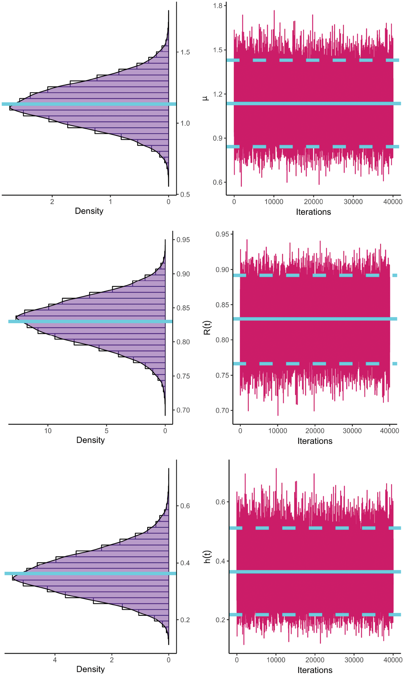
Figure 7: The MCMC plots of μ (top), R(t) (center), and h(t) (bottom) using Sample 𝒮1 from RMM data

6.2 Ball Bearings Data

In this part, we analyze real data representing the times 22 ball bearings (BBs) rotated before they stopped after one million rotations; see Table 15. Caroni [30] and Elshahhat et al. [31] examined this dataset. To examine the superiority of the CJ model, using the BBs data set, the suggested CJ distribution will be compared to the XL, XG, M, L, and E lifetime models. Table 16 indicates that the CJ model is the best compared to others due to having the smallest values for all fitted criteria except the highest p-value. Fig. 8 supports this conclusion also.

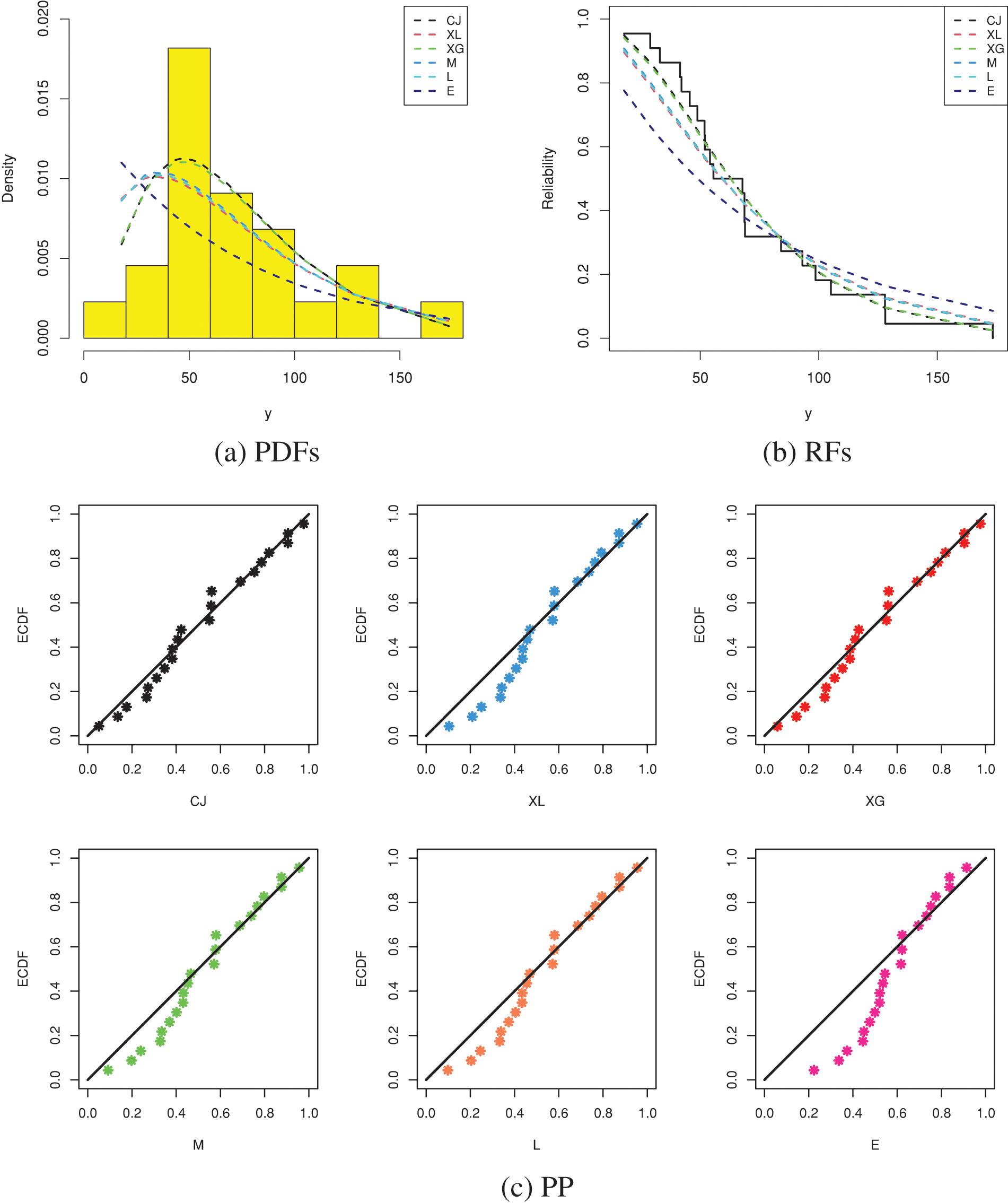
Figure 8: Fitting plots from BBs data

Just like the same estimation scenarios illustrated in Subsection 6.1, from the complete BBs data, different G-PHC samples with fixed (m,r)=(12,8) and various choices of Ri, i=1,…,m are created; see Table 17. However, in Table 18, all estimations results of μ, R(t), and h(t) (at t=1) developed from the likelihood and Bayes’ inferential approaches are presented. However, Table 18 indicates that the acquired point estimates of μ, R(t), or h(t) are quite close to one another. A similar conclusion is reached when comparing the estimated intervals for the same parameters.

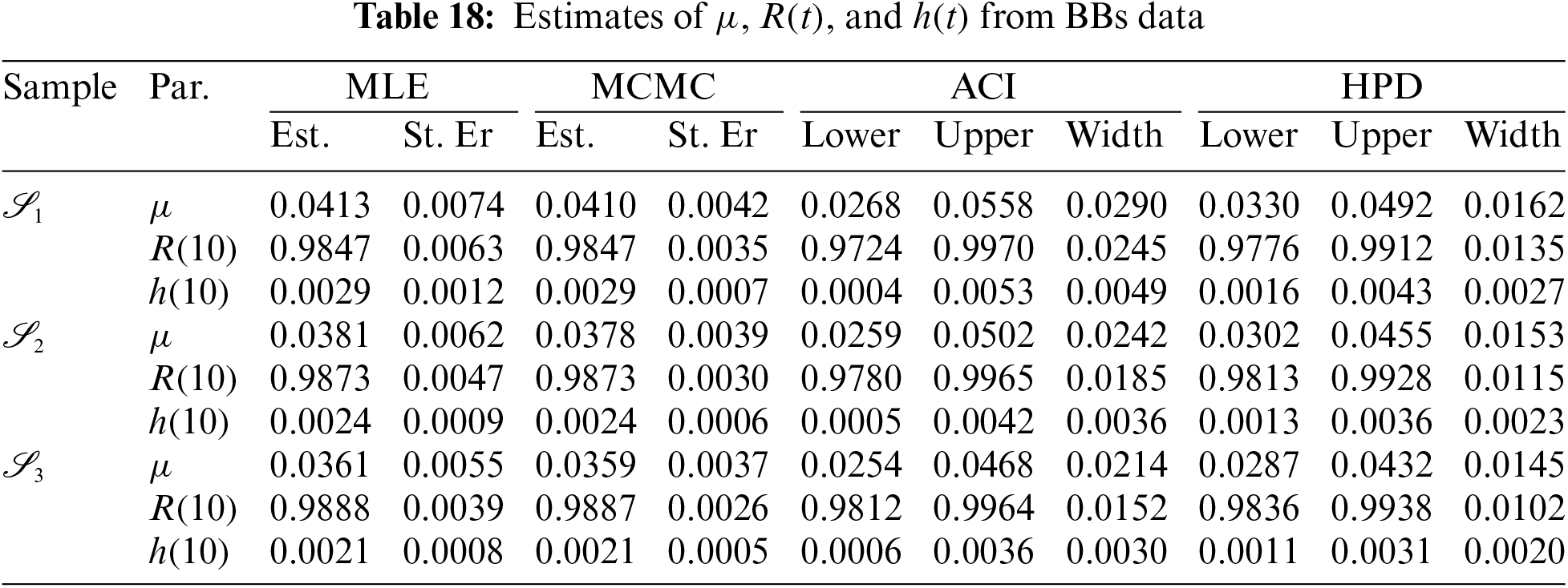
Fig. 9 indicates that the acquired estimates μ^, from 𝒮i, for i=1,2,3, existed and are unique. It also confirms the same results in Table 18. Fig. 10, based on 𝒮1 (as an example), shows that the MCMC algorithm is implemented well and the calculated estimates of μ, R(t), and h(t) are symmetric, negative-skewed, and positive-skewed, respectively.

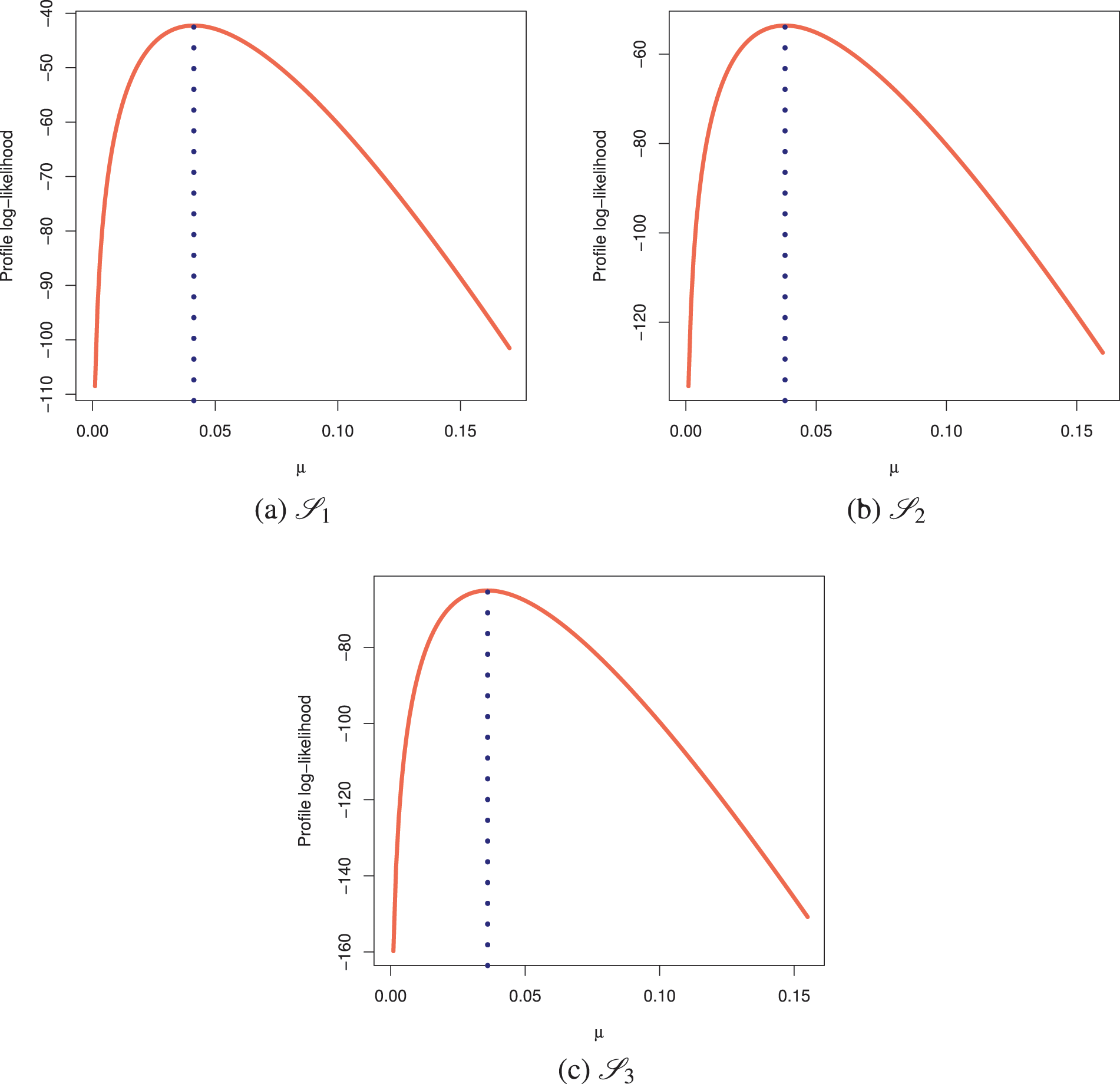
Figure 9: Profile log-likelihoods of μ from BBs data

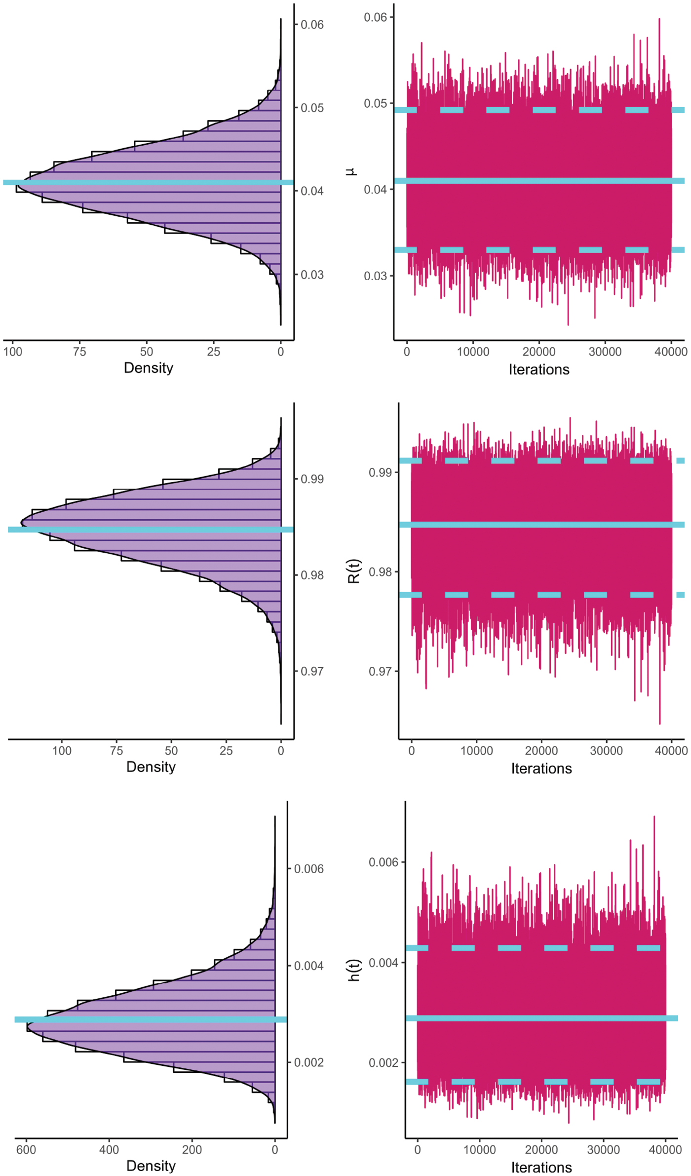
Figure 10: The MCMC plots of μ (top), R(t) (center), and h(t) (bottom) using Sample 𝒮1 from BBs data

As a result of the G-PHC mechanism, the analysis outcomes from the RMM and BBs data sets comprehensively investigate the Chris-Jerry lifetime model, support the simulation results, and demonstrate the feasibility of the proposed operations in the context of an engineering scenario.

7  Conclusions

In this study, we investigated different statistical operations for a novel Chris-Jerry distribution using generalized progressively hybrid censored data. Using both maximum likelihood and Bayesian techniques, we explore the model parameter, reliability, and hazard rate functions. The asymptotic characteristics of the frequentist estimates are used to estimate their asymptotic confidence intervals. The gamma prior distribution and squared error loss are incorporated to provide Bayesian estimation. It comes to light that the posterior distribution cannot be directly determined. Therefore, to get the Bayes’ point/interval investigations, the Markov Chain Monte Carlo approach is used. Various scenarios in an extensive Monte Carlo simulation are used to see the behavior of the various approaches and illustrate their applicability. We noticed that the proposed sampling strategy improves conventional and progressive hybrid censoring processes by allowing an examination to go beyond a predetermined inspection time if scarce failures are collected. The simulation findings revealed that, based on such censored data, the Bayesian technique should be used to estimate Chris-Jerry parameters of life. Real data analysis based on repairable mechanical equipment and ball bearing data sets demonstrated that the suggested model behaved better than numerous other traditional models, including XLindley, Lindley, Xgamma, Muth, and exponential distributions. We focused primarily on the Chris-Jerry lifespan in the context of generalized progressively hybrid data. It would also be interesting to look into the estimate of the same distribution parameters in the presence of a competing risk framework or an accelerated life test. The maximum product of the spacing technique and Bayes’ inference through the spacing-based function may also be considered in future research. Further, it is important to compare the proposed symmetric Bayesian method with the asymmetric Bayesian method against Linex, entropy losses, or others. Moreover, the proposed strategy can be discussed in the presence of fault identification and ball bearing diagnosis data; for further details, we refer to Wu et al. [32]. We believe that the findings and techniques presented in this study will be useful to researchers when the recommended strategy is required.

Acknowledgement: None.

Funding Statement: This research was funded by Princess Nourah bint Abdulrahman University Researchers Supporting Project Number (PNURSP2024R50), Princess Nourah bint Abdulrahman University, Riyadh, Saudi Arabia.

Author Contributions: The authors confirm contribution to the paper as follows: study conception and design: R. A., H. R., A. E.; data collection: R. A., A. E.; analysis and interpretation of results: A. E.; draft manuscript preparation: R. A., H. R. All authors reviewed the results and approved the final version of the manuscript.

Availability of Data and Materials: The data that support the findings of this study are available within the paper.

Conflicts of Interest: The authors declare that they have no conflicts of interest to report regarding the present study.

References

1. Onyekwere CK, Obulezi OJ. Chris-Jerry distribution and its applications. Asian J Probability Stat. 2022;20(1):16–30. doi:10.9734/AJPAS/2022/v20i130480 [Google Scholar] [CrossRef]

2. Balakrishnan N, Kundu D. Hybrid censoring: models, inferential results and applications. Comput Stat Data Anal. 2013;57(1):166–209. doi:10.1016/j.csda.2012.03.025 [Google Scholar] [CrossRef]

3. Balakrishnan N, Cramer E. The art of progressive censoring. Birkhäuser, New York, USA: Springer; 2014. [Google Scholar]

4. Kundu D, Joarder A. Analysis of Type-II progressively hybrid censored data. Comput Stat Data Anal. 2006;50(10):2509–28. doi:10.1016/j.csda.2005.05.002 [Google Scholar] [CrossRef]

5. Cho Y, Sun H, Lee K. Exact likelihood inference for an exponential parameter under generalized progressive hybrid censoring scheme. Stat Methodol. 2015;23:18–34. doi:10.1016/j.stamet.2014.09.002 [Google Scholar] [CrossRef]

6. Henningsen A, Toomet O. maxLik: a package for maximum likelihood estimation in R. Comput Stat. 2011;26:443–58. doi:10.1007/s00180-010-0217-1 [Google Scholar] [CrossRef]

7. Plummer M, Best N, Cowles K, Vines K. CODA: convergence diagnosis and output analysis for MCMC. R News. 2006;6:7–11. [Google Scholar]

8. Koley A, Kundu D. On generalized progressive hybrid censoring in presence of competing risks. Metrika. 2017;80:401–26. doi:10.1007/s00184-017-0611-6 [Google Scholar] [CrossRef]

9. Elshahhat A. Parameters estimation for the exponentiated Weibull distribution based on generalized progressive hybrid censoring schemes. Am J Appl Math Stat. 2017;5(2):33–48. doi:10.12691/ajams-5-2-1 [Google Scholar] [CrossRef]

10. Wang L. Inference for Weibull competing risks data under generalized progressive hybrid censoring. IEEE Trans Reliab. 2018;67(3):998–1007. doi:10.1109/TR.2018.2828436 [Google Scholar] [CrossRef]

11. Lee SO, Kang SB. Estimation for the half-logistic distribution based on generalized progressive hybrid censoring. J Korean Data Inf Sci Soc. 2018;29(4):1049–59. doi:10.7465/jkdi.2018.29.4.1049 [Google Scholar] [CrossRef]

12. Lee K. Bayesian and maximum likelihood estimation of entropy of the inverse Weibull distribution under generalized Type-I progressive hybrid censoring. Commun Stat Appl Methods. 2020;27(4):469–86. doi:10.29220/CSAM.2020.27.4.469 [Google Scholar] [CrossRef]

13. Zhu T. Statistical inference of Weibull distribution based on generalized progressively hybrid censored data. J Computat Appl Math. 2020;371:112705. doi:10.1016/j.cam.2019.112705 [Google Scholar] [CrossRef]

14. Singh DP, Lodhi C, Tripathi YM, Wang L. Inference for two-parameter Rayleigh competing risks data under generalized progressive hybrid censoring. Qual Reliab Eng Int. 2021;37(3):1210–31. doi:10.1002/qre.2791 [Google Scholar] [CrossRef]

15. Elshahhat A, Abu El Azm WS. Statistical reliability analysis of electronic devices using generalized progressively hybrid censoring plan. Qual Reliab Eng Int. 2022;38(2):1112–30. doi:10.1002/qre.3058 [Google Scholar] [CrossRef]

16. Maswadah M. Improved maximum likelihood estimation of the shape-scale family based on the generalized progressive hybrid censoring scheme. J Appl Stat. 2022;49(11):2825–44. doi:10.1080/02664763.2021.1924638 [Google Scholar] [PubMed] [CrossRef]

17. Alotaibi R, Elshahhat A, Nassar M. Analysis of Muth parameters using generalized progressive hybrid censoring with application to sodium sulfur battery. J Radiat Res Appl Sci. 2023;16(3):100624. doi:10.1016/j.jrras.2023.100624 [Google Scholar] [CrossRef]

18. Greene WH. Econometric analysis. 4th ed. New York, NY, USA: Prentice-Hall; 2000. [Google Scholar]

19. Arnold BC, Press SJ. Bayesian inference for Pareto populations. J Econ. 1983;21(3):287–306. doi:10.1016/0304-4076(83)90047-7 [Google Scholar] [CrossRef]

20. Asadi S, Panahi H, Anwar S, Lone SA. Reliability estimation of Burr Type III distribution under improved adaptive progressive censoring with application to surface coating. Maintenance Reliability/Eksploatacja i Niezawodnosc. 2023;25(2):163054. doi:10.17531/ein/163054 [Google Scholar] [CrossRef]

21. Nagy M, Bakr ME, Alrasheedi AF. Analysis with applications of the generalized Type-II progressive hybrid censoring sample from Burr Type-XII model. Math Probl Eng. 2022;2022:1–21. doi:10.1155/2022/1241303 [Google Scholar] [CrossRef]

22. Chen MH, Shao QM. Monte Carlo estimation of Bayesian credible and HPD intervals. J Comput Graph Stat. 1999;8:69–92. doi:10.2307/1390921 [Google Scholar] [CrossRef]

23. Nassar M, Elshahhat A. Estimation procedures and optimal censoring schemes for an improved adaptive progressively type-II censored Weibull distribution. J Appl Stat. 2023. doi:10.1080/02664763.2023.2230536 [Google Scholar] [PubMed] [CrossRef]

24. Murthy DP, Xie M, Jiang R. Weibull models. In: Wiley series in probability and statistics. Hoboken, NJ, USA: Wiley; 2004. [Google Scholar]

25. Chouia S, Zeghdoudi H. The XLindley distribution: properties and application. J Stat Theory Appl. 2021;20(2):318–27. doi:10.2991/jsta.d.210607.001 [Google Scholar] [CrossRef]

26. Sen S, Maiti SS, Chandra N. The xgamma distribution: statistical properties and application. J Mod Appl Stat Methods. 2016;15(1):774–88. doi:10.22237/jmasm/1462077420 [Google Scholar] [CrossRef]

27. Irshad MR, Maya R, Arun SP. Muth distribution and estimation of a parameter using order statistics. Stat. 2021;81(1):93–119. doi:10.6092/issn.1973-2201/9432 [Google Scholar] [CrossRef]

28. Ghitany ME, Atieh B, Nadarajah S. Lindley distribution and its application. Math Comput Simul. 2008;78(4):493–506. doi:10.1016/j.matcom.2007.06.007 [Google Scholar] [CrossRef]

29. Tomy L, Jose M, Veena G. A review on recent generalizations of exponential distribution. Biometr Biostat Int J. 2020;9(4):152–6. doi:10.15406/bbij.2020.09.00313 [Google Scholar] [CrossRef]

30. Caroni C. The correct “ball bearings” data. Lifetime Data Anal. 2002;8:395–9. doi:10.1023/A:1020523006142 [Google Scholar] [PubMed] [CrossRef]

31. Elshahhat A, Bhattacharya R, Mohammed HS. Survival analysis of Type-II Lehmann Fréchet parameters via progressive Type-II censoring with applications. Axioms. 2022;11(12):700. doi:10.3390/axioms11120700 [Google Scholar] [CrossRef]

32. Wu Y, Liu X, Wang YL, Li Q, Guo Z, Jiang Y. Improved deep PCA and Kullback-Leibler divergence based incipient fault detection and isolation of high-speed railway traction devices. Sustain Energy Technol Assess. 2023;57:103208. doi:10.1016/j.seta.2023.103208 [Google Scholar] [CrossRef]