DOI:10.32604/jnm.2022.030178
| Journal of New Media DOI:10.32604/jnm.2022.030178 | |
| Article |
Microphone Array-Based Sound Source Localization Using Convolutional Residual Network
1School of Information and Communication Engineering, Nanjing Institute of Technology, Nanjing, 211167, China
2University of Oulu, Oulu, 90014, FI, Finland
*Corresponding Author: Xiaoyan Zhao. Email: xiaoyanzhao@njit.edu.cn
Received: 20 March 2022; Accepted: 15 April 2022
Abstract: Microphone array-based sound source localization (SSL) is widely used in a variety of occasions such as video conferencing, robotic hearing, speech enhancement, speech recognition and so on. The traditional SSL methods cannot achieve satisfactory performance in adverse noisy and reverberant environments. In order to improve localization performance, a novel SSL algorithm using convolutional residual network (CRN) is proposed in this paper. The spatial features including time difference of arrivals (TDOAs) between microphone pairs and steered response power-phase transform (SRP-PHAT) spatial spectrum are extracted in each Gammatone sub-band. The spatial features of different sub-bands with a frame are combine into a feature matrix as the input of CRN. The proposed algorithm employ CRN to fuse the spatial features. Since the CRN introduces the residual structure on the basis of the convolutional network, it reduce the difficulty of training procedure and accelerate the convergence of the model. A CRN model is learned from the training data in various reverberation and noise environments to establish the mapping regularity between the input feature and the sound azimuth. Through simulation verification, compared with the methods using traditional deep neural network, the proposed algorithm can achieve a better localization performance in SSL task, and provide better generalization capacity to untrained noise and reverberation.
Keywords: Convolutional residual network; microphone array; spatial features; sound source localization
With the development of artificial intelligence, sound source localization (SSL) based on speech processing systems has become a new research hotspot. The task of SSL is to obtain the position information of a sound source relative to an array by processing the sound signal which collected by a sensor when the sound source is unknown. Typical applications of sound source localization technology include: video conferencing, robot hearing, speech enhancement, speech recognition, etc. [1–3].
After years of development, there are more theories and methods in regard to sound source localization based on microphone arrays, and the traditional methods can be classified into three categories: time difference of arrivals (TDOA) estimation methods, steered response power beamforming methods [4], and high-resolution spectral estimation methods. Among them, TDOA estimation methods based on generalized cross correlation (GCC) [5] are widely used because of the small computational power, however the performance degrades significantly in noisy environments. The steered response power (SRP)-based method [6] estimates the sound source location by searching the peak of the spatial power spectrum, where the phase-transform weighted SRP-PHAT based algorithm [7] has better robust performance in the reverberant environment. Spectral estimation techniques have also been applied to multi-source localization, such as methods based on MUSIC [8] and ESPRIT.
All of the above studies are based on traditional algorithms to achieve SSL. Recently, SSL based on supervised learning have been proposed, and the majority of the approaches utilize deep neural networks (DNNs). In [9], a multilayer perceptron deep neural network (DNN) is presented for direction of arrival (DOA) estimation. In [10,11], a convolutional neural network (CNN)-based SSL framework is proposed. In [12], SSL based on time-frequency masking framework and deep learning have been proposed. Yu et al. [13] applied deep neural networks (DNNs) to location-based stereo speech separation. Chakrabarty et al. [14] applied CNNs to microphone array-based sound source localization, the input is the phase components of the short-time Fourier transform (STFT). Adavanne et al. [15] proposed a DOAnet network to achieve SSL based on microphone array, with the input to the DOAnet being the magnitude and phase components of the STFT. Unsupervised learning [16] and semi-supervised learning methods based on manifold learning [17] have also been used in various studies, as well as deep generative modeling [18].
Traditional sound source localization techniques are fail to achieve satisfactory performance in adverse noisy and reverberant environments. The structure of ResNet introduced into the convolutional residual network (CRN) model can reduce feature loss and decrease the training difficulty. Research shows that when the DRN model is similar to the CNN model in terms of the number of layers, the CRN model not only has a rapid drop in loss function during training and good model convergence performance, but also has better performance. Therefore, we propose a method using CRN to improve localization performance. The spatial features including TDOAs between microphone pairs and SRP-PHAT spatial spectrum are extracted in each Gammatone sub-band. The spatial features of different sub-bands with a frame are combine into a feature matrix as the input of CRN. Simulation verified that compared with the methods using traditional deep neural network, the proposed algorithm can achieve a better localization performance in SSL task, and provide better generalization capacity to untrained noise and reverberation.
The remainder of the paper is laid out as follows. Section 2 illustrates the CRN-based SSL algorithm, which includes four sections with the overview of system, extraction of feature parameters, CRN architecture and the training of CRN. Section 3 formulates the experimental results and analyses, and conclusions are stated in Section 4.
2 Sound Source Localization Algorithm Using CRN
As illustrated in Fig. 1, the localization framework is divided into the training phase and the testing phase, and the system input is made up of the signals received by the microphone array. The Gammatone filter is used to decompose the signals into sub-band. The TDOA and SRP-PHAT spatial spectrum are calculated within the sub-band, and then combined into spatial feature matrix as the input of CRN network. In the training phase, the CRN network is used to construct the mapping law between the spatial feature matrix and the source azimuth; in the localization phase, the trained CRN model is used to predict the probability of the tested signal belonging to each azimuth, with the highest probability being selected as the estimated azimuth.
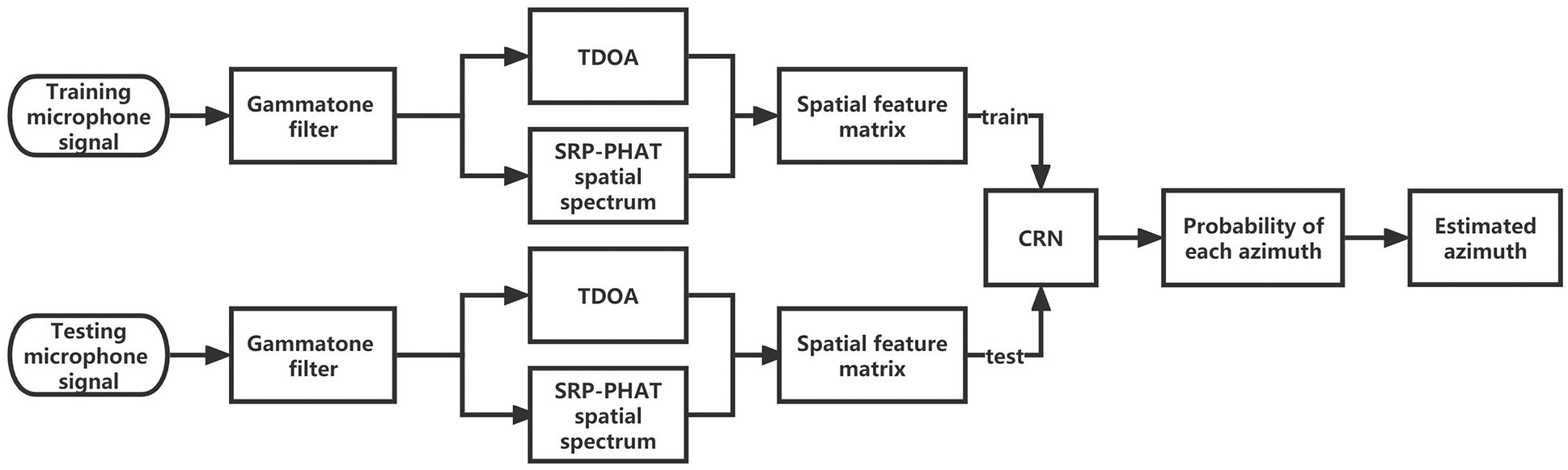
Figure 1: Block diagram of the proposed sound source localization system
The model of microphone array received signals can be expressed as:
where t is the time serial number, “*” represents convolutional operations, hm(rs, t) denotes the room impulse response from the source position rs to the mth microphone, vm(t) is the corresponding noise interference term. Furthermore, the source position, microphone position and acoustic environment have significant effect on the hm(rs, t).
The Gammatone filter is used to decompose the signals into sub-band, whose expression can be written as:
where c is the gain coefficient, n means the order of the filter, bi and fi represent the decay coefficient and central frequency of the ith filter respectively.
GCC function within the Gammatone sub-band is calculated as:
where i is the ith Gammatone sub-band, k is the frame number, and Xm(k, ω) is the short-time Fourier transform of xm(t). Therefore, the TDOA between the mth and nth microphone in ith sub-band can be expressed as follows:
The number of microphones is M, so there are
The SRP-PHAT within the Gammatone sub-band is expressed as:
τ(r) denotes the difference in propagation delay from the steering position r.
In a given frame, the TDOA and SRP-PHAT of all sub-band form a spatial feature matrix, and that can be calculated as follows:
where I denotes the number of sub-band, L denotes the number of steering positions. Moreover, in this paper, I is 32, L is 36, and M is 6. Therefore, the dimension of the localization clues in each sub-band is 15 + 36 = 51, and the dimension of the feature matrix E(k) is 51 × 32.
The structure of the CRN model used in this paper is depicted in Fig. 2, as well as the structure of residual block is illustrated in Fig. 3. It can be seen that the residual block is composed of several convolutional layers and batch normalization (BN) layers. In this paper, each residual block structure contains two BN layers and two convolutional layers, and the input signal is processed in the order of BN, ReLU activation, and convolutional operation. From Fig. 3, each residual block includes two BN layers and two convolutional layers, for a total of four network layers. From Fig. 2, the block diagram of CRN model structure includes two residual block, and this equal to eight network layers, in addition to one pooling layer and two fully connected layer. Considering the input layer and the output layer, the CRN network used in this paper has a total of thirteen layers. In the CRN model, the size of the convolution kernel in each residual block is 3 × 3, the step size is 1 × 1, and the output of convolution is zero-filled to keep the same dimension. The number of implied units in the first fully connected layer is 128, and the number of implied units in the second fully connected layer is 36 corresponding to the number of output azimuths. The output layer uses Softmax and the loss function is the cross-entropy loss function.

Figure 2: Block diagram of CRN model structure
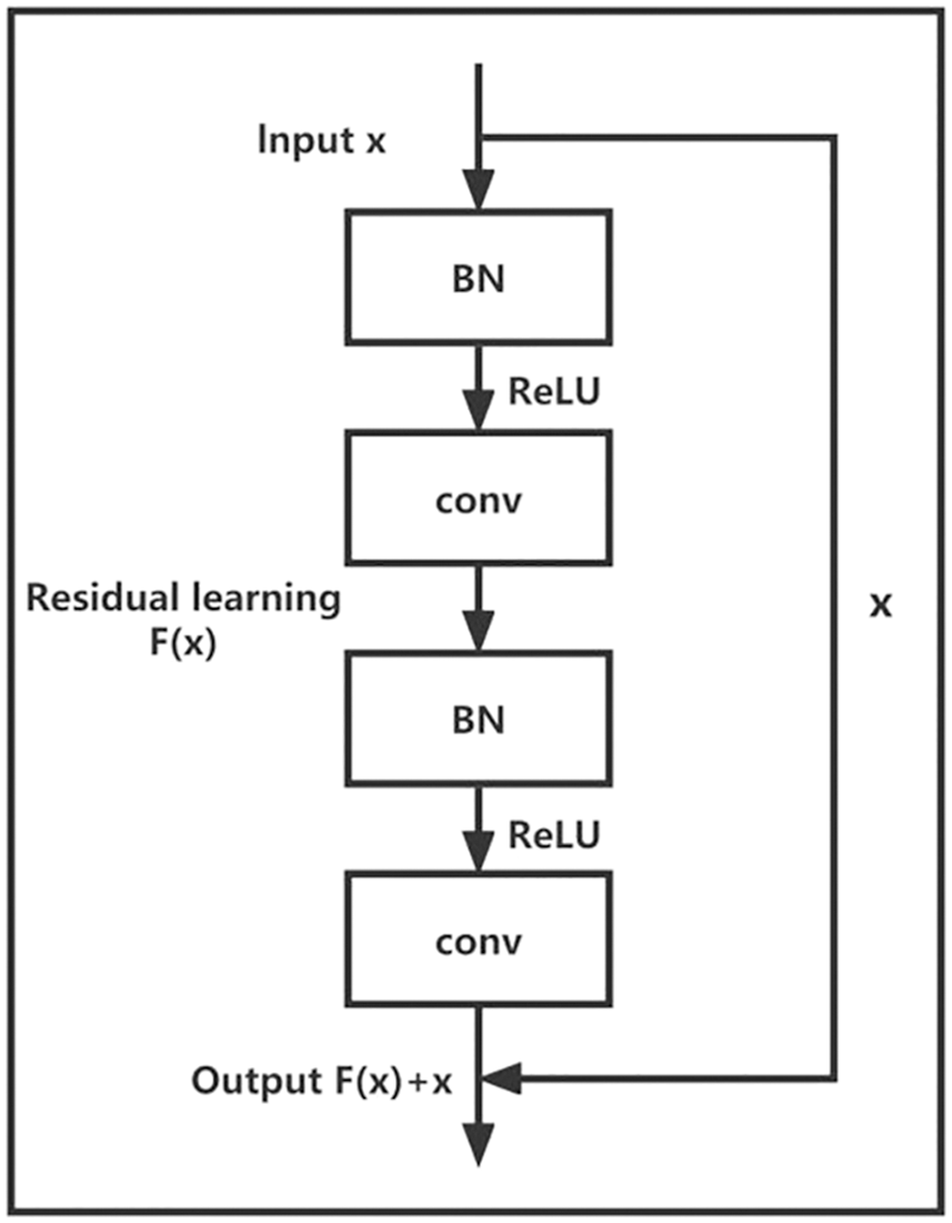
Figure 3: Structure of residual block
In this paper, the Adam optimizer is used during the training process. During the training process, information is propagated forward and errors are propagated backward, and the model parameters are updated accordingly. The initial learning rate is 0.001, and the amount of batch data 200. Moreover, the value of ε in the BN layer is set to 0.001, and the decay coefficient is taken to be 0.999. Outstanding parameter initialization will make the network training easier. We use Xavier to initialize the parameters, which automatically adjusts to the most appropriate distribution according to the number of input and output nodes in the network layer, thus making the parameters moderate in size. The cross-validation approach divides the training data into 70% training sets and 30% validation sets at random.
3 Simulation and Result Analysis
The simulated room’s dimensions are stated as 7 m × 7 m × 3 m. A uniform circular array which consists of six omnidirectional microphones with a diameter of 0.2 m is placed in (3.5, 3.5, 1.6 m). The clean speech sampled with 16 kHz which are adopted as sound source signals are taken at random from the TIMIT database. Between any two positions, the image method generates the room impulse response. By convolving the clean sound source signal with the ambient impulse response and adding uncorrelated Gaussian white noise, the microphone signal is generated. Then, divide the microphone signals into 32-ms frames and window using the Hamming window. Windowing of the framed signals can reduce the truncation effect between signal frames and reduces spectral leakage.
The source is placed in the far-field, and the distance between the array and the training position is adjusted to 1.5 m, with a training azimuth range of 0° to 360° in 10° steps. During the training phase, SNR is set to five scenarios: 0, 5, 10, 15 and 20 dB, and T60 has two set values: 0.5 and 0.8 s. The training data is derived via combining microphone signals in various reverberation and noise environments during the training stage for robustness.
The proposed algorithm’s performance is compared to three baseline methods, SRP-PHAT [7], SSL-DNN [19] and SSL based on convolutional neural network (SSL-CNN) [11]. The percentage of correct estimates is an essential criterion in our assessment of SSL performance, which can obtained as:
where Nall denotes the total number of test frames, nc represents the number of correct estimate frames.
3.2 Evaluation in Setup-Matched Environments
In this section, we compare and analyse the performance of different algorithm in the same setting of training and testing.
As shown in Fig. 4, the performance of SRP-PHAT degrades dramatically when SNR declines and reverberation duration grows, and indeed the proposed algorithm’s performance is significantly outstanding than the SRP-PHAT algorithm. As the proposed algorithm exploits the combination of the Gammatone sub-band TDOA and SRP-PHAT as a feature matrix, and adopts a CRN model that introduces a ResNet structure reducing the training difficulty and accelerating the model convergence. Moreover, the proposed algorithm’s performance improvement is the greatest when comparing to the SRP-PHAT algorithm at roughly SNR = 10 dB in the same reverberant environment. Furthermore, in the same SNR scenario, the performance improvement of the proposed algorithm is greater than that of the SRP-PHAT algorithm at higher reverberation duration.
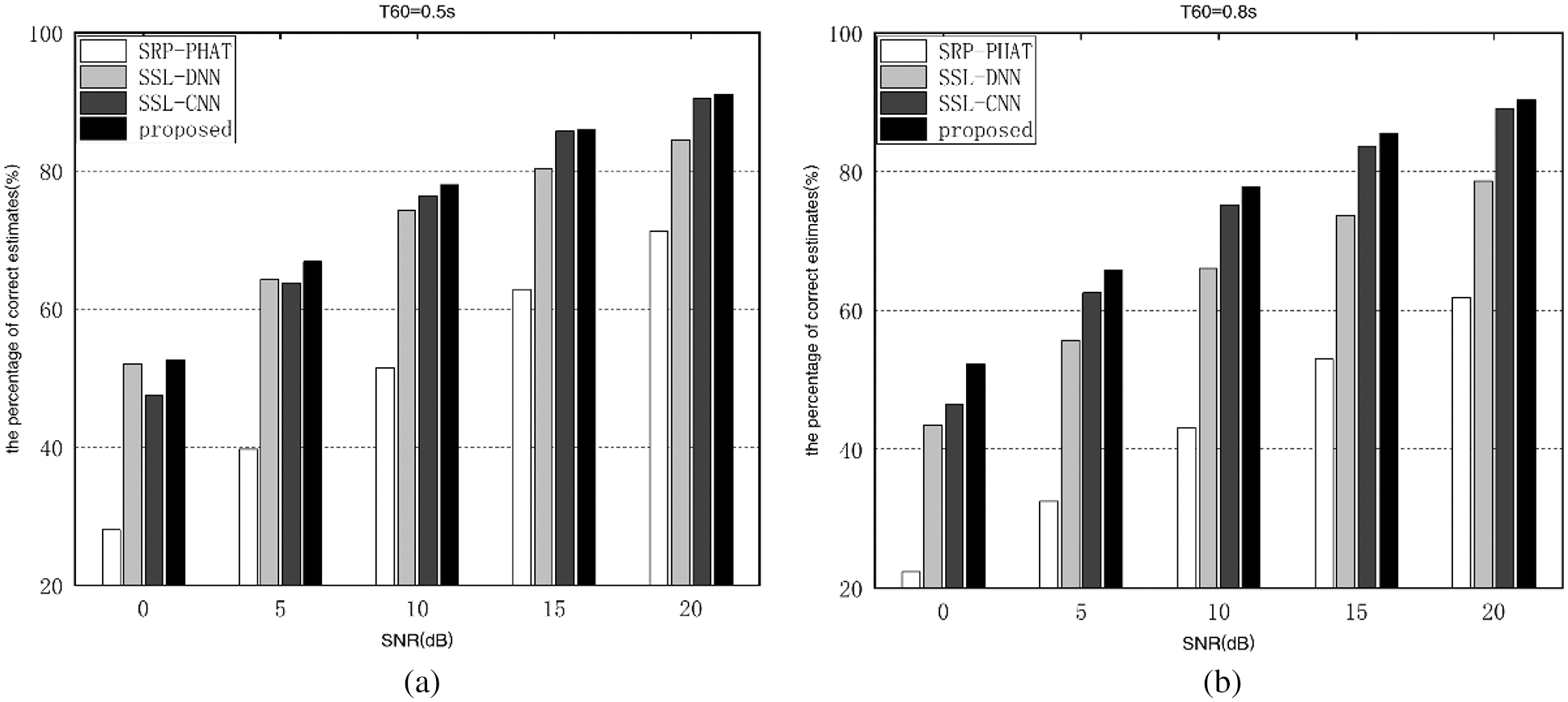
Figure 4: Percentage of correct estimates of different algorithms in setup-matched environments. (a) T60 = 0.5 s (b) T60 = 0.8 s
As shown in Fig. 4, in all situations, the proposed algorithm is significantly better than the SSL-DNN algorithms and SSL-CNN algorithms. Moreover, the superiority of the proposed algorithm is particularly evident at higher reverberation time. Furthermore, as SNR increases, the proposed algorithm’s performance improvement increases gradually compared to the SSL-DNN algorithm, and the proposed algorithm’s performance improvement decreases gradually compared to the SSL-CNN algorithm in the same reverberant environment. For instance, in the scenario of T60 = 0.8 s, when the SNR grows from 0 to 20 dB, compared to the SSL-DNN algorithm, the proposed algorithm’s percentage of correct estimations increases from 8.73% to 11.69%. In the same situation, the performance improvement decreases from 5.66% to 1.27% compared to the SSL-CNN algorithm.
3.3 Evaluation in Setup-Unmatched Environments
In this section, we compare and analyse the performance of different algorithm in the different settings of training and testing. The untrained SNR is set to five scenarios: 0, 5, 10, 15 and 20 dB, and the untrained reverberation time T60 has two set values: T60 = 0.6 s and T60 = 0.9 s. Figs. 5 and 6 illustrate performance comparisons of different algorithms in untrained noise environment and untrained reverberation environment respectively.

Figure 5: Percentage of correct estimates of different algorithms in untrained noise environments. (a) T60 = 0.5 s (b) T60 = 0.8 s
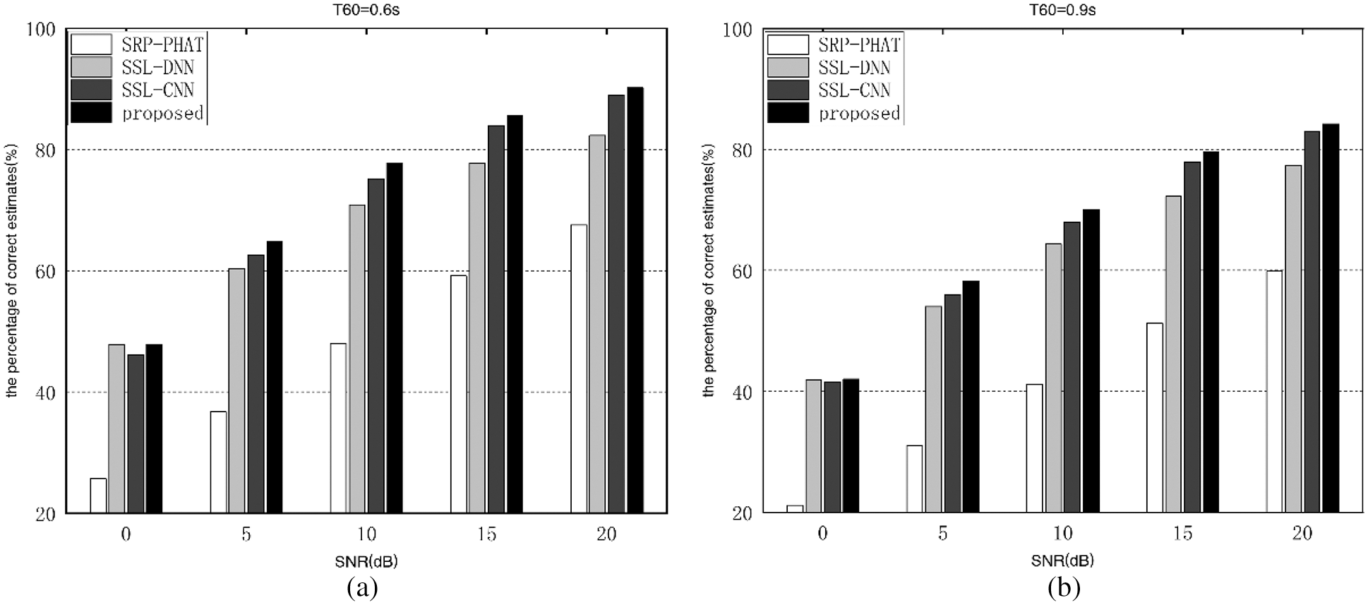
Figure 6: Percentage of correct estimates of different algorithms in untrained reverberation environments. (a) T60 = 0.6 s (b) T60 = 0.9 s
As shown in Fig. 5, compared to the SRP-PHAT algorithm, the proposed algorithm’s performance improvement is the most distinctive at 8 dB of SNR in the untrained and the same reverberant environment. For instance, in the scenario of T60 = 0.8 s, when the SRN goes from −2 to 8 dB, the performance improvement increases from 22.2% to 31.55%. In addition, as the SNR climbs from 8 to 18 dB, it decreases from 31.55% to 26.26%. What’s more, in the same SNR scenario, the proposed algorithm’s performance improvement is more dramatically at higher reverberation time.
As illustrated in Figs. 5 and 6, we find that data fluctuation in the untrained setting with regularity, and similar to that stated in Section 3.2, indicating that the proposed algorithm in this paper is extremely robust and general to untrained noise and reverberation. Particularly, the percentage of correct localization estimates is improved by 28% compared to the SRP-PHAT algorithm. Compared with the SSL-DNN algorithm, in the environments of low SNR, the proposed algorithm have similar localization performance with SSL-DNN algorithm, with the percentage of correct localization estimates improving from about 4% to 10% in both trained and untrained environments. Compared to the SSL-CNN algorithm, the percentage of correct localization estimates improves from about 3% to 4% in both trained and untrained environments.
In the paper, a novel CRN-based SSL algorithm is proposed. In the proposed algorithm, TDOAs between microphone pairs and SRP-PHAT spatial spectrum in Gammatone sub-band are extracted as spatial features. Since CRN introduces residual structures based on convolutional networks, it reduces the difficulty of the training process and accelerates the convergence of the model. Experimental data express that the proposed algorithm achieves improved performance of localization and more robust against noise and reverberation.
Acknowledgement: The authors would like to show their deepest gratitude to the anonymous reviewers for their constructive comments to improve the quality of the paper.
Funding Statement: This work is supported by Nature Science Research Project of Higher Education Institutions in Jiangsu Province under Grant No. 21KJB510018, National Nature Science Foundation of China (NSFC) under Grant No. 62001215.
Conflicts of Interest: The authors declare that they have no conflicts of interest to report regarding the present study.
1. B. Yang, H. Liu and C. Pang, “Multiple sound source counting and localization based on TF-wise spatial spectrum clustering,” IEEE/ACM Transactions on Audio, Speech, and Language Processing, vol. 27, no. 8, pp. 1241–1255, 2019. [Google Scholar]
2. M. Jia, J. Sun and C. Bao, “Real-time multiple sound source localization and counting using a soundfield microphone,” Journal of Ambient Intelligence and Humanized Computing, vol. 8, no. 6, pp. 829–844, 2017. [Google Scholar]
3. J. Dávila-Chacón, J. Liu and S. Wermter, “Enhanced robot speech recognition using biomimetic binaural sound source localization,” IEEE Transactions on Neural Networks and Learning Systems, vol. 30, no. 1, pp. 138–150, 2019. [Google Scholar]
4. W. L. Shi, Y. S. Li and L. Zhao, “Controllable sparse antenna array for adaptive beam forming,” IEEE Access, vol. 7, pp. 6412–6423, 2019. [Google Scholar]
5. Z. Q. Wang, X. L. Zhang and D. L. Wang, “Robust TDOA estimation based on time-frequency masking and deep neural networks,” in 19th Annual Conf. of the Int. Speech Communication, Hyderabad, India, pp. 322–326, 2018. [Google Scholar]
6. D. Yook, T. Lee and Y. Cho, “Fast sound source localization using two-level search space clustering,” IEEE Transactions on Cybernetics, vol. 46, no. 1, pp. 20–26, 2016. [Google Scholar]
7. Y. Wu, R. Ayyalasomayajula, M. J. Bianco, D. Bharadia and P. Gerstoft, “Sslide: Sound source localization for indoors based on deep learning,” in IEEE ICASSP, Toronto, ON, Canada, pp. 4680–4684, 2021. [Google Scholar]
8. M. Jia, S. Gao and C. Bao, “Multi-source localization by using offset residual weight,” EURASIP Journal on Audio, Speech, and Music Processing, vol. 23, no. 2021, pp. 1–18, 2021. [Google Scholar]
9. X. Xiao, S. Zhao, X. Zhong, D. L. Jones, E. S. Chng et al., “A learning-based approach to direction of arrival estimation in noisy and reverberant environments,” in IEEE ICASSP, South Brisbane, QLD, Australia, pp. 2814–2818, 2015. [Google Scholar]
10. S. Chakrabarty and E. A. P. Habets, “Multi-speaker DOA estimation using deep convolutional networks trained with noise signals,” IEEE J. Sel. Topics Signal Process, vol. 13, no. 1, pp. 8–21, 2019. [Google Scholar]
11. X. Y. Zhao, L. Zhou and Y. Tong, “Robust sound source localization using convolutional neural network based on microphone array,” Intelligent Automation & Soft Computing, vol. 30, no. 1, pp. 361–371, 2021. [Google Scholar]
12. Z. Q. Wang, X. Zhang and D. L. Wang, “Robust speaker localization guided by deep learning-based time-frequency masking,” IEEE/ACM Transactions on Audio, Speech, and Language Processing, vol. 27, no. 1, pp. 178–188, 2018. [Google Scholar]
13. Y. Yu, W. Wang and P. Han, “Localization based stereo speech source separation using probabilistic time-frequency masking and deep neural networks,” EURASIP Journal on Audio, Speech, and Music Processing, vol. 2016, no. 1, pp. 7–12, 2016. [Google Scholar]
14. S. Chakrabarty and E. A. P. Habets, “Broadband DOA estimation using convolutional neural networks trained with noise signals,” IEEE Workshop on Applications of Signal Processing to Audio and Acoustics (WASPAA), vol. 2017, no. 10, pp. 136–140, 2017. [Google Scholar]
15. S. Adavanne, A. Politis and T. Virtanen, “Direction of arrival estimation for multiple sound sources using convolutional recurrent neural network,” in 26th Signal Processing Conf. (EUSIPCO), Rome, Italy, pp. 1462–1466, 2018. [Google Scholar]
16. R. Takeda and K. Komatani, “Unsupervised adaptation of deep neural networks for sound source localization using entropy minimization,” in IEEE ICASSP, New Orleans, LA, USA, pp. 2217–2221, 2017. [Google Scholar]
17. B. Laufer-Goldshtein, R. Talmon and S. Gannot, “Semi-supervised sound source localization based on manifold regularizatio,” IEEE/ACM Transactions on Audio, Speech, and Language Processing, vol. 24, no. 8, pp. 1393–1407, 2016. [Google Scholar]
18. M. J. Bianco, S. Gannot and P. Gerstoft, “Semi-supervised source localization with deep generative modeling,” in IEEE 30th Int. Workshop on Machine Learning for Signal Processing (MLSP), Espoo, Finland, pp. 1–6, 2020. [Google Scholar]
19. X. Y. Zhao, S. W. Chen and L. Zhou, “Sound source localization based on SPR-PHAT spatial spectrum and deep neural network,” Computers, Materials & Continua, vol. 64, no. 1, pp. 253–271, 2020. [Google Scholar]
 | This work is licensed under a Creative Commons Attribution 4.0 International License, which permits unrestricted use, distribution, and reproduction in any medium, provided the original work is properly cited. |