DOI:10.32604/biocell.2022.016625
| BIOCELL DOI:10.32604/biocell.2022.016625 | |
| Article |
BDLR: lncRNA identification using ensemble learning
1Jiangsu Key Lab of Big Data Security & Intelligent Processing School of Computer Science, Nanjing University of Posts and Telecommunications, Nanjing, 210046, China
2Smart Health Big Data Analysis and Location Services Engineering Laboratory of Jiangsu Province, Nanjing, 210046, China
3Zhejiang Engineering Research Center of Intelligent Medicine, Wenzhou, 325035, China
4College of Computer Science and Technology, Nanjing Forestry University, Nanjing, 210037, China
*Address correspondence to: Lejun Gong, glj98226@163.com
Received: 12 March 2021; Accepted: 25 May 2021
Abstract: Long non-coding RNAs (lncRNAs) play an important role in many life activities such as epigenetic material regulation, cell cycle regulation, dosage compensation and cell differentiation regulation, and are associated with many human diseases. There are many limitations in identifying and annotating lncRNAs using traditional biological experimental methods. With the development of high-throughput sequencing technology, it is of great practical significance to identify the lncRNAs from massive RNA sequence data using machine learning method. Based on the Bagging method and Decision Tree algorithm in ensemble learning, this paper proposes a method of lncRNAs gene sequence identification called BDLR. The identification results of this classification method are compared with the identification results of several models including Byes, Support Vector Machine, Logical Regression, Decision Tree and Random Forest. The experimental results show that the lncRNAs identification method named BDLR proposed in this paper has an accuracy of 86.61% in the human test set and 90.34% in the mouse for lncRNAs, which is more than the identification results of the other methods. Moreover, the proposed method offers a reference for researchers to identify lncRNAs using the ensemble learning.
Keywords: lncRNAs; High-throughput sequencing; Ensemble learning; Bagging; Decision Tree
In the human genome, scientists have found that about 2% of the total genome can encode proteins (Pennisi, 2012). Many DNA is transcribed into RNA but not translated into proteins, these non-coding RNAs are called ncRNAs (Djebali et al., 2012). Common ncRNAs include tRNA, snRNA, rRNA, snoRNA, lncRNA, Small ncRNA and so on. Among them, long non-coding RNAs (lncRNAs) are a class of RNA molecules whose sequence length is more than 200 nucleotides (Bu et al., 2012; Derrien et al., 2012), lacking specificity and complete open reading frame, and no protein coding ability. Scientists previously thought that only genes encoding proteins can play an important role in various life activities. They only need to use these genes as the focus of scientific research, but ignore the function of lncRNAs, they believe that such molecules are “junk substances” that do not play any role in life activities. In recent years, massive biomedical data have shown that lncRNAs play an important role in many life activities, such as epigenetic regulation, cell cycle regulation, dosage compensation and cell differentiation regulation. LncRNAs regulate DNA methylation, histone modification, chromatin remodeling and other forms of RNA interference through a variety of pathways. As an important component of the eukaryotic transcriptome, lncRNAs have been shown to be associated with many diseases such as cancer (Cheetham et al., 2013; Wapinski and Chang, 2011), AIDS (Eilebrecht et al., 2011), heart failure (Li et al., 2013). Recognition and inclusion of lncRNAs will help researchers to further study and explore human diseases at the molecular level. Accurate identification of lncRNAs is an important step to further understand long non-coding RNA.
With the rapid development of computing technology, predicting new lncRNAs using bioinformatics methods has become a hotspot in RNA genomics. However, biological experimental methods have some limitations in identifying and annotating long non-coding RNAs, such as the low expression levels of most lncRNAs and the challenge of massive experimental data analysis (Vučićević et al., 2014). With the development of next generation sequencing technology, millions of transcript sequence data are generated every year. A large number of lncRNAs have been discovered and many lncRNAs have been annotated in the transcriptome, which makes it possible to identify from massive RNA sequences using machine learning. The machine learning method can combine a variety of gene sequence features to construct a classifier for identifying lncRNAs and new input lncRNAs sequences. Support Vector Machine (Cutler et al., 2007; Schneider et al., 2017), Logical Regression (Hoo et al., 2016; Xie et al., 2018), Decision Tree (Gong et al., 2017; Sun et al., 2015) and other supervised learning methods have been used to identify lncRNAs.
After investigating the related methods of identifying lncRNAs, it is found that there are few methods to construct classifier to identify lncRNAs using Bagging method in ensemble learning. Therefore, this paper proposes a method based on Bagging and Decision tree to identify LncRNAs named BDLR. The method uses the ID3 Decision Tree algorithm as the base learner and uses the Bagging method in ensemble learning to combine multiple base learners (Decision Trees) to obtain the BDLR classifier. In this paper, three types of features are extracted from highly reliable data: k-mer frequency, GC content, and transcript length. The classification results of BDLR method are compared with the results of Support Vector Machine, Logistic Regression and Decision Tree. The experimental results show that the identification effect of BDLR classifier based on ensemble learning is better than that of the other three classifiers.
Therefore, the proposed BDLR method is promising for the identification and annotation of lncRNAs sequences.
In this section, we first introduce the source of the experimental data, then introduce the features used in the BDLR method and the method of feature selection. Then we discuss the related algorithms used in the BDLR classification model proposed in this paper, and finally describe the construction process of the BDLR classification model. There are three types of features used in BDLR: k-mer subsequence frequency, GC content, transcript sequence length. The chi-square test is used to select the optimal feature subset.
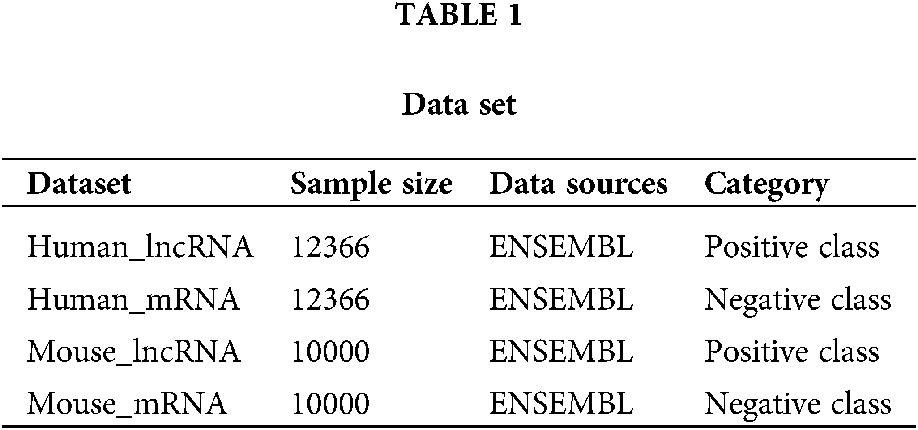
At present, human biomedical experimental data and gene annotation information are relatively abundant. Many genomic databases contain a large number of human lncRNAs and mRNAs (a common class of protein-coding transcripts) sequence data, such as ENSEMBL, NONCODE, GENCODE (Derrien et al., 2012) genomic databases. This paper uses two types of data sets. The sequencing data of LncRNA and mRNA were obtained from ENSEMBL genomic database for both human and mouse data sets. The human positive dataset used in this paper is the human lncRNAs sequence downloaded from the ENSEMBL genomic database. After filtering out the sequence of less than 200 nucleotides in length, 12366 lncRNA sequences were obtained. The negative dataset was also obtained from the ENSEMBL genomic database. The human mRNAs sequence, after filtering out the sequence of less than 200 nucleotides in length, obtained a total of 61427 mRNA sequences. In order to ensure the relative balance of the number of positive and negative samples, 12366 mRNA sequences were randomly selected from the 61427 mRNA sequences as negative data. Experimental data related to mouse are similar to those of humans downloaded from ENSEMBL genomic database. LncRNA were filtered with 10000 lncRNA sequences and 10000 mRNA sequences. The data set information is shown in Table 1. The data set in this work is balanced, but there may be unbalanced data set in the real world. For such unbalanced data set, we will preprocess it by up-sampling or down-sampling, so that it can process unbalanced data set.
(1) K-mer subsequence frequency
K-mer usually refers to all subsequences of a sequence whose length is k (Zhang et al., 2011). In bioinformatics, k-mer refers to all k-length subsequences in a DNA or RNA sequence or to all k-length subsequences in an amino acid sequence. The frequency features of k-mer subsequences mainly use the k-mer statistical information to discover the distribution of the frequency of the k-mer subsequence in the RNA sequence or the amino acid sequence. The feature of k-mer frequency is also presented in the work (Li et al., 2019).
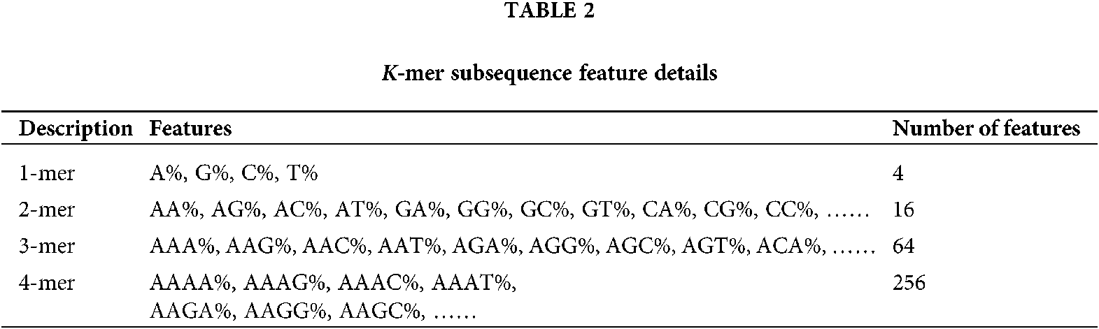
According to the characteristics of the k-mer, a sliding window strategy can be adopted to calculate the frequency of the k-mer subsequences in each RNA sequence. The step size of the sliding window is set to 1, that is, the window moves one base position to the right each time. For a RNA sequence of length L, let k be a value range of k = 1, 2, 3, ……, n, because the base at each position of k-mer subsequence in RNA sequence can be any of the four bases A, T, C and G, there are 4k possible combinations of k-mer subsequences of length k, so the total number of k-mer frequency features is: 41+42+43+……+4n. A sliding window of width 1 requires scanning the RNA sequence k times, and each scan can obtain L-k+1 k-mer subsequences. As shown in Fig. 1 below, a schematic diagram of the k-mer subsequence contained in the position of the sliding window corresponding to the same width at k, 2, 3, and 4 in the RNA sequence.

Figure 1: Sketch of k-mer sliding window.
In this paper, the range of k is limited to k = 1, 2, 3 and 4, a total of 4 + 16 + 64 + 256 = 340 k-mer frequency features can be extracted. Details are shown in Table 2. For a RNA sequence with length L, the sliding window needs to be scanned four times, and each scan will get mk = L – k + 1 k-mer subsequence; each scan will increase the corresponding number of k-mer subsequences ni by 1, ni means the number of occurrences of the i-th k-mer subsequence; then the frequency of occurrence of each k-mer subsequence Fi = ni/mk. The i-th feature extracted is represented by Fi, and the specific calculation formula is as formulas (1) and (2).
k = 1, 2, 3, 4; i = 1, 2, 3, 4, ……, 340;
Fi: the frequency of the i-th k-mer subsequence;
ni: the number of occurrences of the i-th k-mer subsequence in the current RNA;
mk: the number of k-mer subsequences obtained by scanning the RNA sequence for the kth time;
L: the length of the currently scanned RNA sequence.
(2) GC content and transcript length
Nucleic acid bases are typically biological compounds found in deoxyribonucleic acid (DNA) and ribonucleic acid (RNA). The bases mainly include adenine (A), thymine (T), cytosine (C) and guanine (G), and the GC content refers to the sum of contents of guanine (G) and cytosine (C) in a gene sequence. In the related research of genomic sequence, GC content (Banerjee et al., 2005; (Singer and Hickey, 2000) is a very important feature. The GC content in DNA double strands of different species is very different. GC content is also related to many genetic characteristics, for example, when GC content is relatively low, the density of genes is relatively small, and when GC content is relatively high, the density of genes is relatively large; GC content also has a large influence on the composition of nucleotides and amino acids. The length of a transcript refers to the length of an RNA sequence (lncRNA or mRNA sequence), and the distribution of lengths of different classes of RNA sequences is also different.
(3) Chi-square test
The chi-square test is a commonly used method of feature selection, especially in the financial and biological fields (Kowal et al., 2018). The chi-square is used to describe the independence between two variables, or to describe the degree of deviation between the observed actual values and the theoretical expectations (Dou and Aliaosha, 2018). The larger the chi-square value, the greater the deviation between the actual value and the expected value, and the weaker the independence between the two variables. The formula for calculating chi-square value (x2) is as follows:
Explanation:
t: when this feature exists, t = 1, and when this feature does not exist, t = 0;
c: category 0 or 1 (this paper only considers the two classifications);
N: observation value;
E: expectations, such as E11, represent expectations when feature t appears and category c = 1 (originally assumed to be independent of t and c).
After the chi-square value is obtained, the chi-square value can be converted into a P-value. The P-value is the probability of sample results when the original hypothesis is true. When the P-value is small, it can be considered that the original hypothesis is wrong, that is, feature t is related to category c. Therefore, chi-square test can be used to rank the correlation degree of features and categories to achieve the purpose of feature selection. Feature selection by chi-square test can reduce the number of features and improve the training speed of the classification model. At the same time, it can reduce the impact of noise features and improve the classification accuracy of the classification model on the test set. In addition, from the perspective of the complexity of the model, it can also reduce the complexity of the model and reduce the possibility of the over-fitting.
Ensemble learning and Decision Tree algorithms
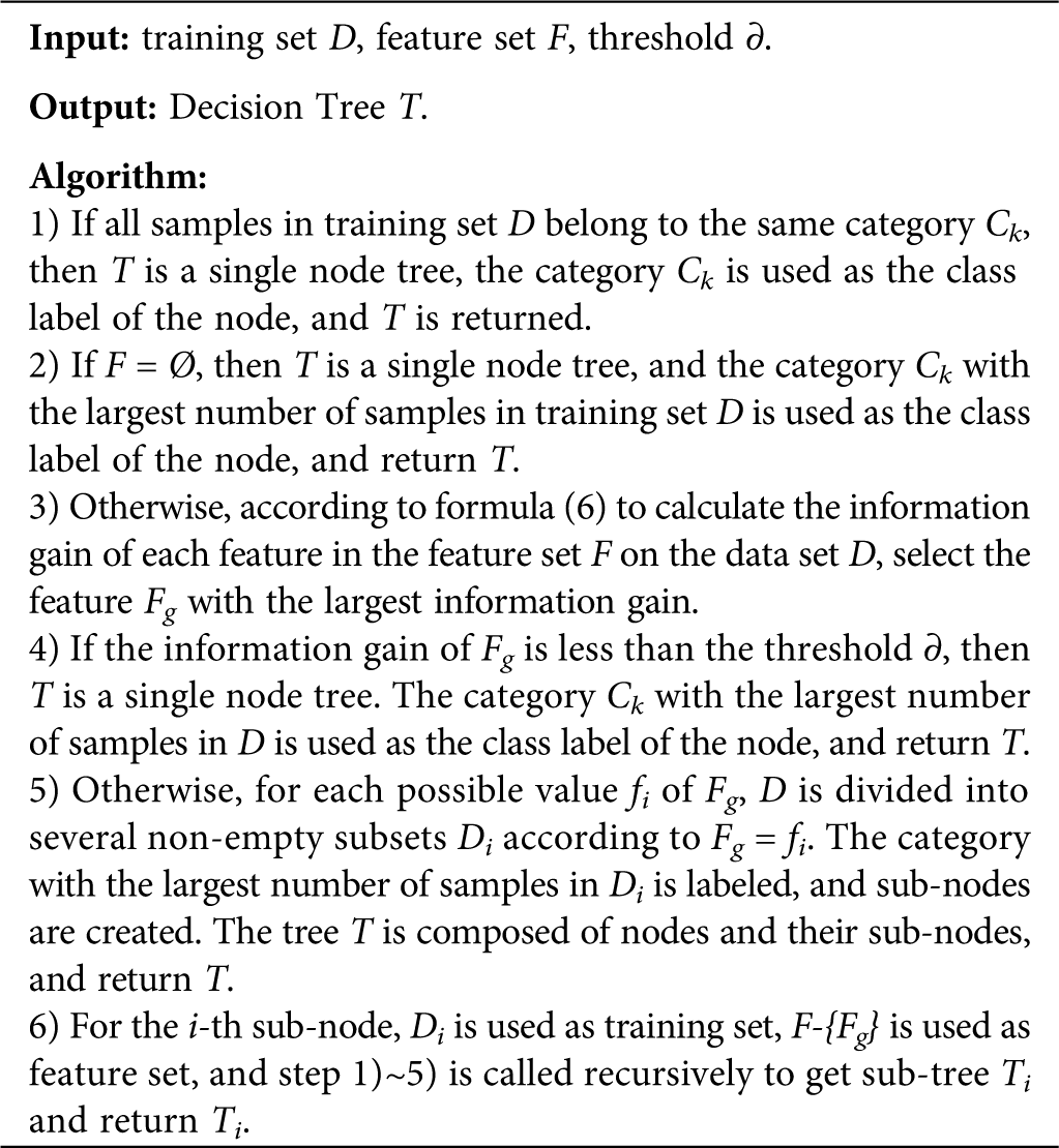
(1) Decision Tree algorithms
In this paper, ID3 Decision Tree algorithm is used as the base learner of Bagging method. ID3 algorithm uses information gain criterion to selects features at each node of the decision tree and constructs the decision tree recursively.
In information theory, entropy is a measure of uncertainty of random variables. The larger the entropy, the greater the uncertainty of the random variable. The definition of entropy is as follows:
X is a random variable,
The conditional entropy H(Y|X) refers to the uncertainty of random variable Y under the condition of given random variable X. Conditional entropy is defined as follows:
In the above formula,
Information gain represents the degree to which the classification uncertainty of data set D decreases when the information of feature F is known. Information gain is defined as follows:
ID3 Decision Tree algorithm (Li, 2012) is described as follows:
(2) Ensemble learning
Ensemble learning achieves better generalization performance than single learner by combining multiple single learners to complete learning tasks together (Xiao et al., 2018; Zhou, 2016). Bagging (Bootstrap Aggregating) is the most famous parallel ensemble learning algorithm (Liu et al., 2018; Zararsız et al., 2017). The basic flow of this algorithm is: given a data set D containing m samples, randomly extract one sample into the sampling set, put the sample back into the original data set D, repeat sampling m times, and get a sampling set D’, which also contains m samples. According to the principle of bootstrap sampling, about two-thirds of the samples in data set D will appear in D’, the remaining one-third of the samples will not appear in D’, and these samples not in D’ can be used as test sets for out-of-bag estimation of generalization performance; repeated T times of the same operation will result in a set of samples whose number is m. T base learners are trained by using the T set. Finally, the classification results of the T base learners are combined according to the strategy of majority voting or averaging, and the final classification results are obtained. The base learner chosen in this paper is Decision Tree. The process of obtaining BDLR classification model is shown in Fig. 2. The Bagging algorithm description (Liu et al., 2018) is as follows:
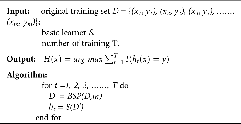
• yi is the real category label of sample xi;
• BSP (D, m) denotes m times of random sampling with playback for data set D;
• I(*) stands for the indicator function. When * is true and false, the value is 1,0, respectively.
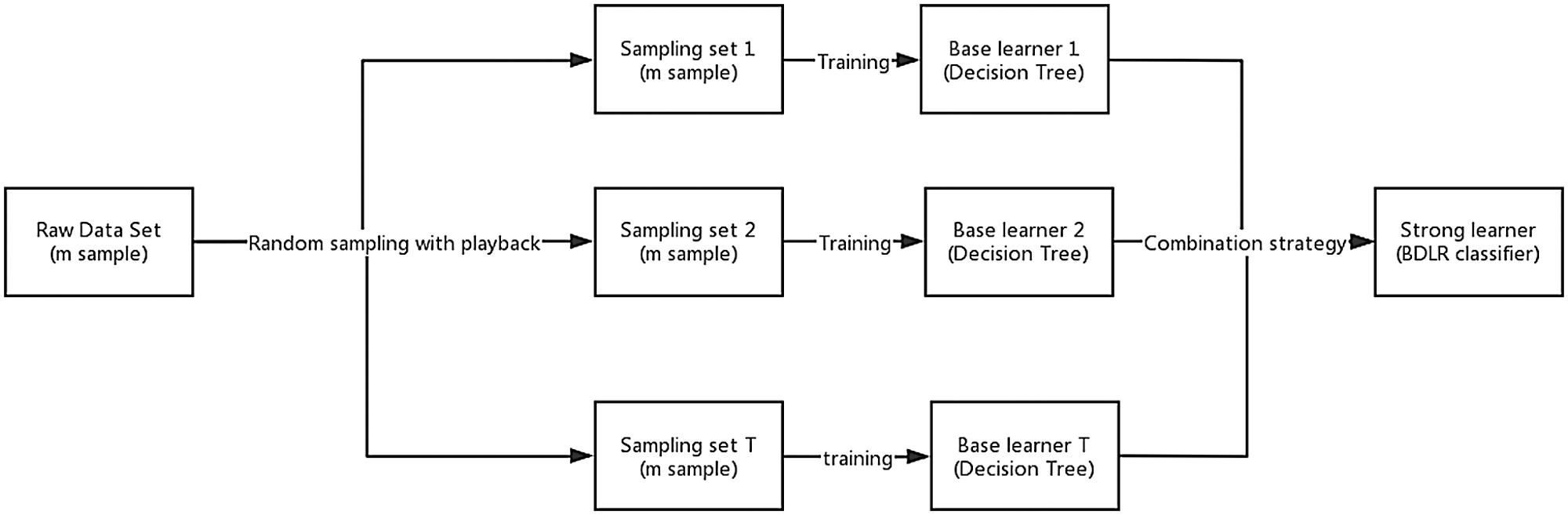
Figure 2: The process of training and integrating multiple decision tree using Bagging method.
Design of lncRNA identification method——BDLR
This paper proposes a method to identify human lncRNA called BDLR, which integrates multiple ID3 Decision Tree algorithms by using Bagging algorithm. BDLR is an algorithm with ensemble learning as its core. In order to obtain generalized ensemble learning, Bagging’s self-help sampling method is adopted to improve the average value of the base classifier of ensemble learning when selecting samples. Decision tree algorithm is often chosen as a base classifier because of its good generalization ability in ensemble learning. Therefore, ID3 decision tree algorithm is selected as the base classifier. The process of identifying human lncRNA using the method is shown in Fig. 3.

Figure 3: Human lncRNA identification process based on BDLR classifier.
The steps for identifying human lncRNA using the BDLR method are described below:
1) Highly reliable lncRNA sequence data and mRNA sequence data were downloaded from ENSEMBL genome database as positive and negative datasets, respectively.
2) The k-mer subsequence frequency, GC content and transcript sequence length were extracted from the downloaded RNA sequence data, and a total of 342 features were obtained.
3) Using chi-square test as feature selection method, the optimal feature subset of a total of 40 features is selected from the initial feature set.
4) Using the ID3 Decision Tree algorithm as a base learner, 50 decision trees are combined using the Bagging method in integrated learning. In this process, the number T of Decision Trees used is compared. The results show that the classification accuracy of BDLR classifier is 86.24% when T = 40, 87.02% when T = 50, 86.30% when T = 60 and 86.29% when T = 500. Therefore, 50 Decision Trees are selected for integration.
5) The accuracy, precision, recall and F1_score obtained by BDLR method are compared with those obtained by other methods to evaluate the advantages and disadvantages of BDLR method.
Performance evaluation metrics
This paper will use Accuracy (ACC), Precision (P), Recall (R), F1_score to evaluate the performance of the classification model. Definitions are as follows:
In the above formula, TP (true positive) refers to the number of samples correctly predicted as positive classes; FN (false negative) refers to the number of samples incorrectly predicted as negative classes; FP (false positive) refers to the number of samples incorrectly predicted as positive classes; TN (true negative) refers to the number of samples correctly predicted as negative classes.
In this section, the optimal feature subset is obtained by analyzing the performance of BDLR classification model on different feature subsets in the two types of datasets (human and mouse). Then the classification performance of BDLR classification model on the test data set is compared. The data set is divided into a training set and a test set with the ratio of 6 to 4 by using the train_test_split function. Using the training data set to solve the hyperparameters (optimal feature subset) of BDLR classification model, The obtained optimal hyperparameters are used in the test set for evaluating the performance of the BDLR against other models.
According to the definition of k-mer subsequence frequency, the frequency values of 340 k-mer subsequences are calculated. Considering the total number of features of k-mer frequency is large, the distribution of some features is calculated by box plot (Streiner, 2018). The frequency distributions of “A%” in partial 1-mer subsequences of lncRNA (left) and mRNA (right) sequences, “GC%” in 2-mer subsequences, “GGG%” in 3-mer subsequences and “GGGG%” in 4-mer subsequences were calculated. It is worth noting that “GC” 2-mer feature and GC-content feature are two completely different features. “GC” 2-mer refers to the frequency of 2-mer base pairs like “AC”, “TC” and “GC” in RNA base pairs. The GC-content feature indicates the ratio of GC content to AT content in the whole RNA. As shown in Fig. 4, it can be found that there are obvious differences in k-mer frequency distribution between the two types of data. Therefore, k-mer subsequence frequency can be used as an important feature to distinguish lncRNA from mRNA.
Similarly, according to the definition of GC content and transcript length (Karimi et al., 2018), GC content and transcript length of lncRNA and mRNA sequences were calculated respectively. In Fig. 5 (left), the GC content distribution of lncRNA and mRNA was compared using a box plot, it can be seen that there is a significant difference in the GC content distribution between the two types of data. In Fig. 5 (right), a statistical analysis of the lncRNA and mRNA sequence lengths using a box plot reveals that there is also a significant difference in the sequence length distribution between the two types of data. In the analysis process, it should be noted that because the RNA sequence has a large range of length distribution, it is necessary to logarithmically transform the initially acquired RNA length data, and to narrow the numerical distribution range of the data, which will be more conducive to our statistical analysis. From the above analysis, GC content and transcript sequence length are also two important features to distinguish lncRNA from mRNA.
The three types of features, k-mer frequency, GC content, and transcript length, were combined to obtain a total feature set of 342 dimensions. It should be noted that the GC content and transcript length should be standardized before merging, so that the range of these two types of features is consistent with the range of k-mer frequency characteristics.
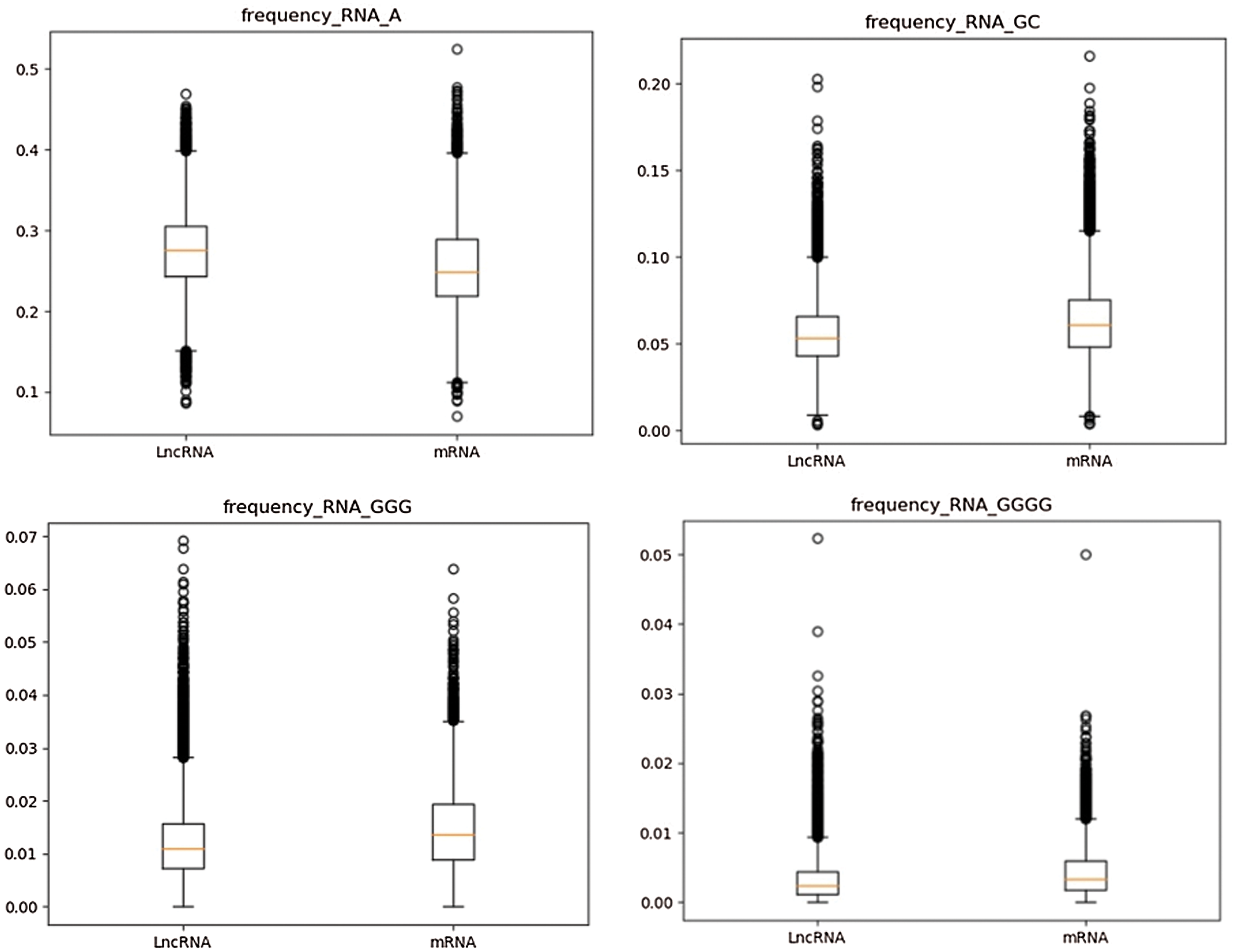
Figure 4: Frequency distribution of partial k-mer subsequences in lncRNA and mRNA.
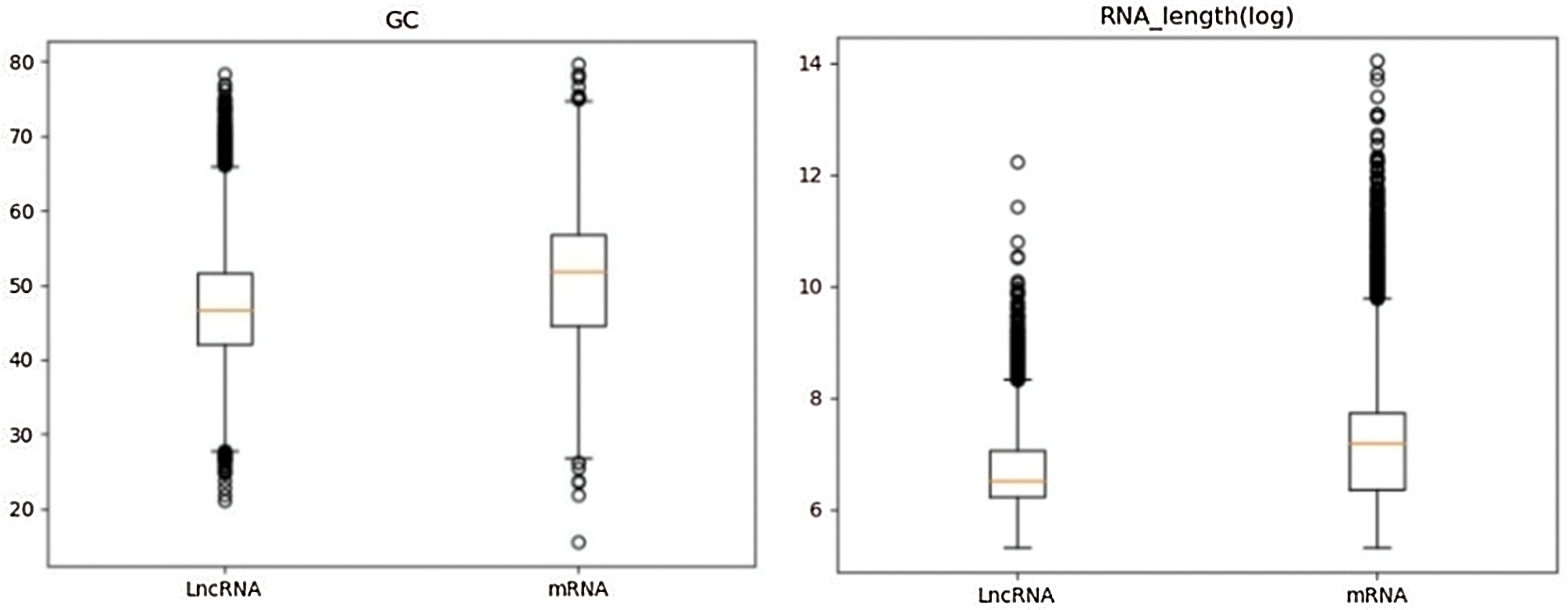
Figure 5: Left: GC content distributions in lncRNA and mRNA; right: Sequence length distributions in lncRNA and mRNA.
The training set is used to select the optimal feature subset. Chi-square test was used to select the initial feature set (Yu et al., 2017), and then the feature subsets with p-value ranking top30, top40, top50 and top100 were selected for comparative analysis. The four feature subsets were selected as input features of BDLR classifier, and the classification results of this method under each feature subset were compared. In the human data set, it was found that BDLR method had the best identification results for lncRNA under top40 feature subset. The classification accuracy of BDLR method under top40 feature subset was 87.02%, higher than that of top30 feature subset 84.85%, higher than that of top50 feature subset 86.48%, and higher than that of top100 feature subset 86.94%. The recall rate and F1_score of BDLR method on top40 feature subset are the highest, with a precision of 87.29% slightly lower than 87.91% of top100 feature subset. However, the training time of BDLR method on top40 feature subset is 28.7 s, which is 1/2 of the training time on top100 feature subset. Considering the classification result of the model and the training time of the model, the top40 feature subset is selected as the optimal feature subset. The human classification results of BDLR classifier under each feature subset are shown in Table 3. In this paper, the same experiment has been done on the mouse data set. Experimental results show that the top 40 feature subset is superior to other feature subsets in Accuracy, Precision, Recall and F1_score. The mouse classification results of BDLR classifier under each feature subset are shown in Table 4. The 40 features in the optimal feature subset of human selected by Chi-square test are shown in Fig. 6 and the optimal feature subset of mouse in Fig. 7. They are also used in the test dataset for measuring the performance of BDLR.
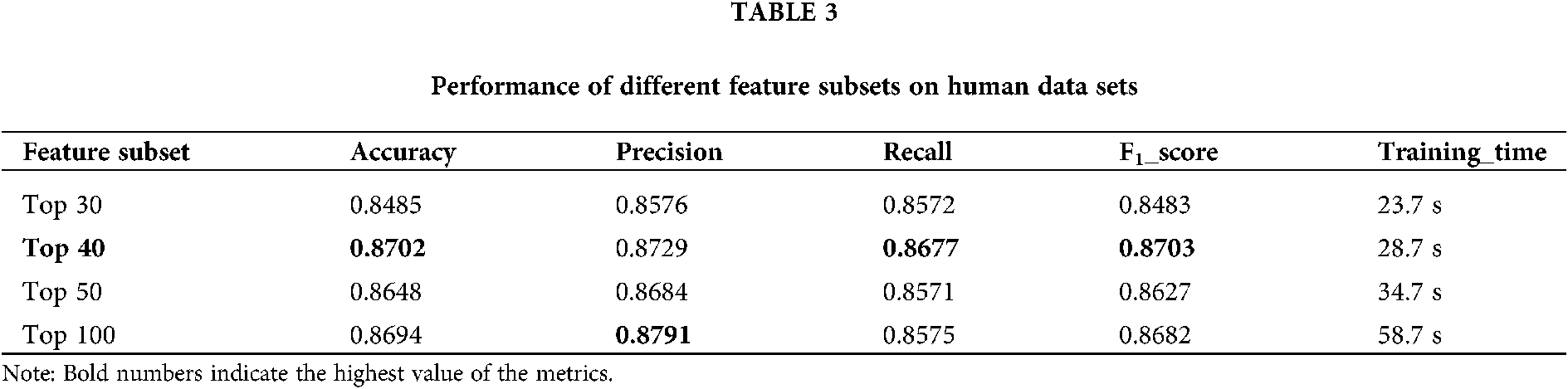
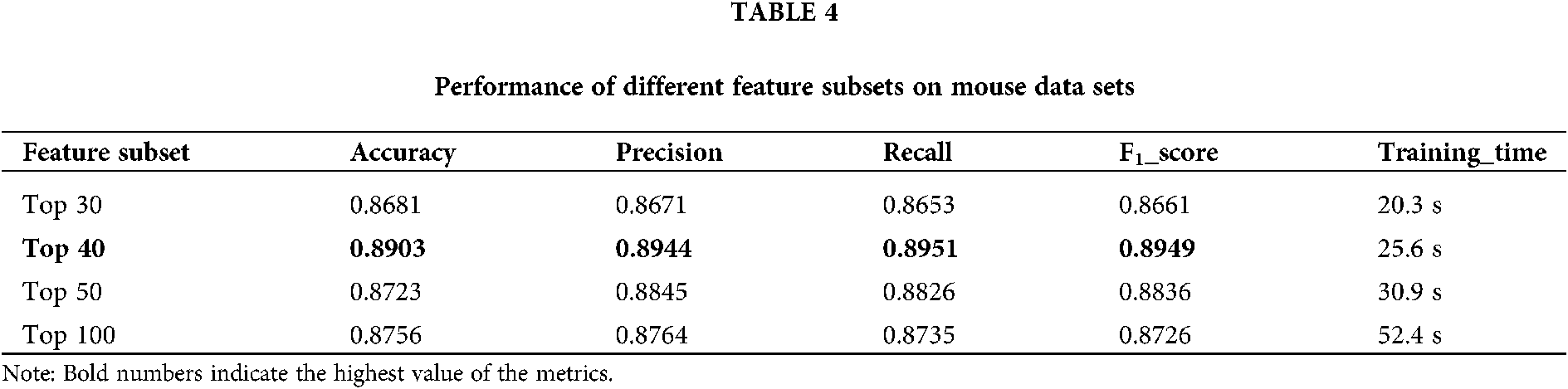
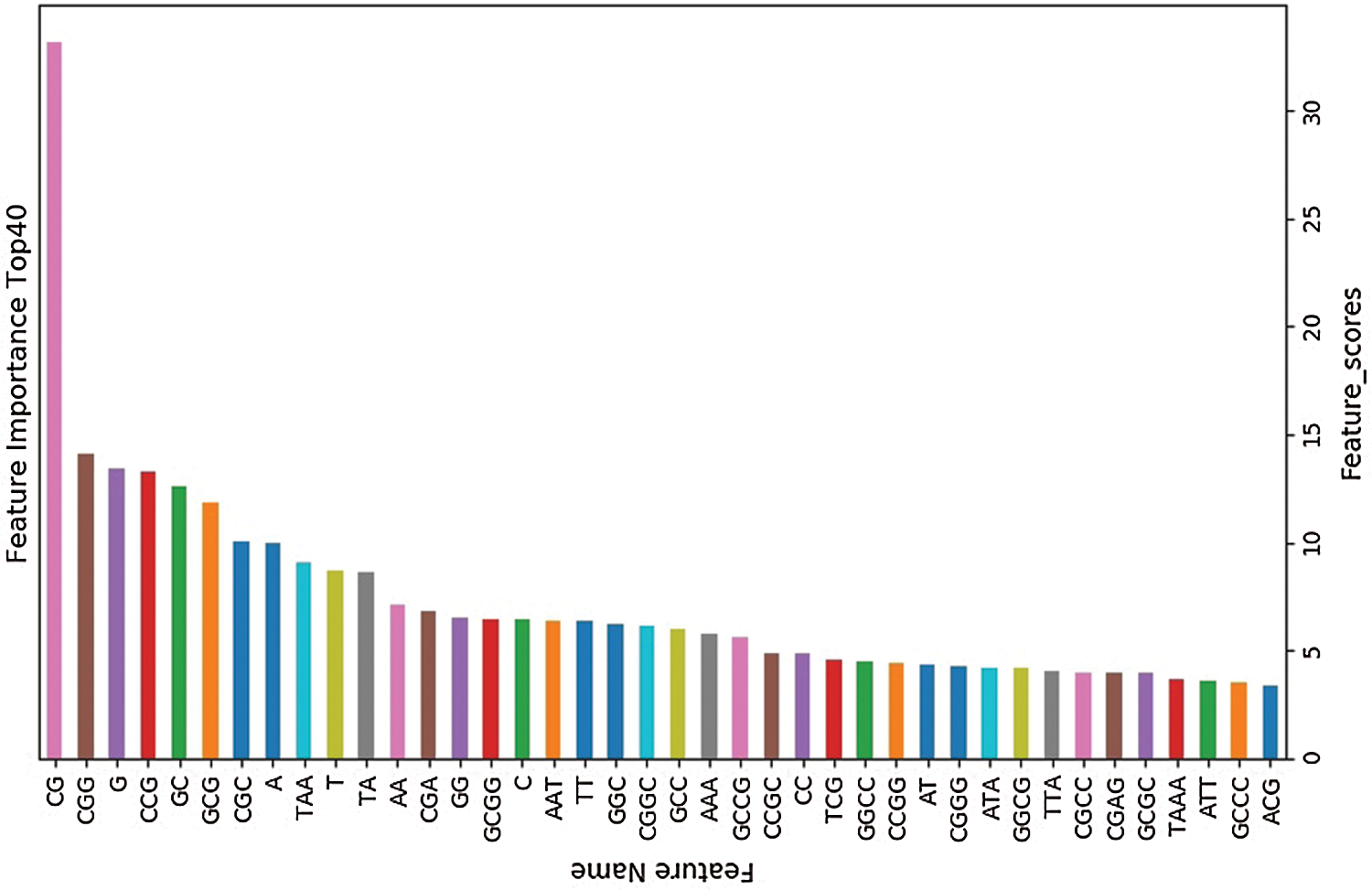
Figure 6: Optimal feature subset (human).
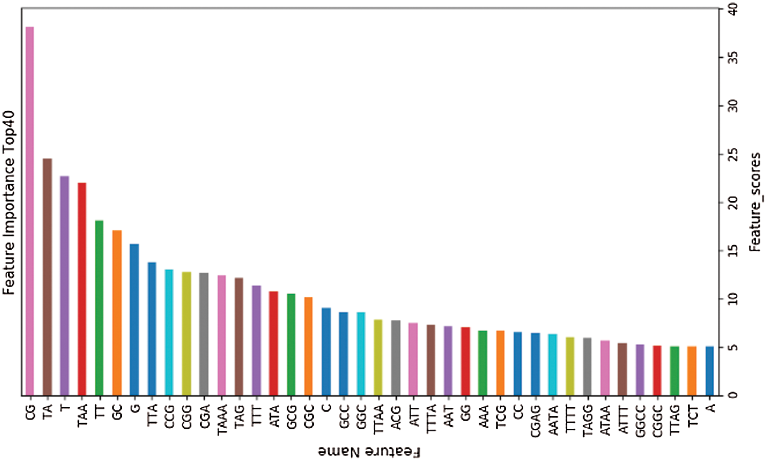
Figure 7: Optimal feature subset (mouse).
Performance evaluation of BDLR classification model
In the human data set, 12366 lncRNA data were taken as positive samples and 12366 mRNA as negative samples. In the mouse data set, 10000 LncRNA data were taken as positive samples and 10000 mRNA as negative samples. Use the train_test_split function to randomly divide it into a training set with size of 0.6 and a test set with size of 0.4. In order to verify the effectiveness of the proposed method, the classification method adopted by some popular lncRNA recognition tools is used to classify the same data set used in this paper, and the results are compared. The classification methods used for comparison include the Logistic Regression (LR) model adopted by CPAT tool (Wang et al., 2013), the Support Vector Machine (SVM) model adopted by CPC tool (Kong et al., 2007), and the Decision Tree (DT) model adopted by the base learner in the BDLR method proposed in this paper and Traditional Byes model (Huai et al., 2015) based on statistical method, RF (Random Forset) (Cutler et al., 2007), which also use ensemble learning method is compared and analyzed (Only the training set is selected for hyperparameters). The comparison results shown in Tables 5 and 6. From the human comparison results, it can be seen that the proposed method is superior to the other classification methods in Accuracy (ACC): 86.61%, Precision (P): 86.62%, Recall (R): 86.61%, F1_score: 86.61%. And, also for the mouse comparison results, it can be seen that the proposed method is also superior to the other classification methods in Accuracy (ACC): 90.34%, Precision (P): 90.35%, Recall (R): 90.35%, F1_score: 90.34%. The classification accuracy of BDLR method proposed in this paper is obviously higher than other compared method. The classification results of BDLR are the best among all the methods, and that of Byes is the worst.


The ROC curves (Hoo et al., 2016) of the seven classification algorithms on the test data are shown in Fig. 8 for human and Fig. 9 for mouse. The BDLR method proposed in this paper has the largest AUC value of 0.94 for human and 0.97 for mouse; the second largest AUC value is the Random Forest, which is 0.91 for human and 0.97 for mouse; the Byes algorithm has the smallest AUC value of 0.69 for human and 0.78 for mouse. Based on the above analysis, the method proposed could effectively identify lncRNA gene sequences.
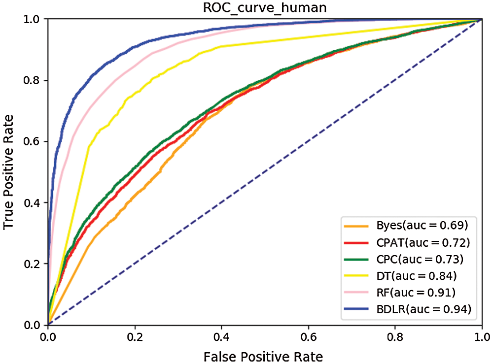
Figure 8: ROC curve for human.
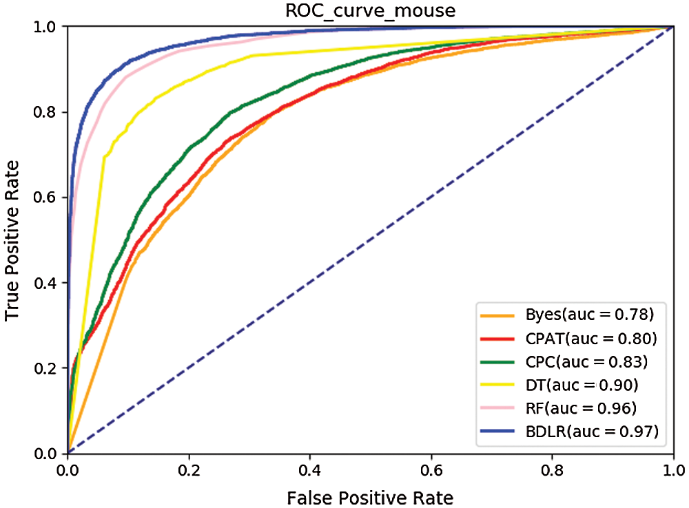
Figure 9: ROC curve for mouse.
In this paper, a lncRNA identification method named BDLR is proposed. Based on human and mouse RNA sequence data, three kinds of features: k-mer subsequence frequency, GC content and transcript sequence length, are extracted. The 342 features are taken as the original feature set, and the optimal feature subset of 40 features is obtained by feature selection method of chi-square test. A lncRNA classification model based on Bagging ensemble learning method was trained. The results show that the classification accuracy of BDLR is 86.61%, AUC value is 0.94 aiming at the human dataset, and the accuracy is 90.34%, AUC value is 0.97 aiming at the mouse data set. The performance of BDLR is higher than Byes, CPAT (Logistic Regression), CPC (SVM), Decision Tree, Random Forest aiming at the same test data set. The ensemble learning method, which is rarely used in the identification of lncRNA to our best knowledge, effectively improves the accuracy and training speed of the traditional machine learning method. Moreover, the proposed method lays a foundation for researchers in related fields to use the ensemble learning method to identify lncRNA. Experiments show that this method has strong generalization ability and can effectively identify human lncRNA, which is of great significance for the identification and annotation of lncRNA. In the future, we could consider combining deep learning to further improve the classification performance of lncRNA.
Availability of Data and Materials: All the data in this paper comes from the open source Ensemble database.
Author Contribution: Study conception and design: Lejun Gong; data collection: Yongmin Li and Shehai Zhou; analysis and interpretation of results: Shehai Zhou, Jingmei Chen and Yongmin Li; draft manuscript preparation: Lejun Gong, Shehai Zhou and Jingmei Chen. Li Zhang and Zhihong Gao checked the manuscript. All authors reviewed the result and approved the final version of the manuscript.
Funding Statement: This work is supported by the National Natural Science Foundation of China (61502243, 61502247, 61572263), China Postdoctoral Science Foundation (2018M632349), Zhejiang Engineering Research Center of Intelligent Medicine under 2016E10011, Foundation of Smart Health Big Data Analysis and Location Services Engineering Lab of Jiangsu Province (SHEL221-001), and Natural Science Foundation of the Higher Education Institutions of Jiangsu Province in China (No. 16KJD520003).
Conflicts of Interest: The authors declare that they have no conflicts of interest to report regarding the present study.
Banerjee T, Gupta S, Ghosh TC (2005). Role of mutational bias and natural selection on genome-wide nucleotide bias in prokaryotic organisms. Biosystems 81: 11–18. [Google Scholar]
Bu D, Yu K, Sun S, Xie C, Skogerbø G et al. (2012). NONCODE v3. 0: Integrative annotation of long noncoding RNAs. Nucleic Acids Research 40: D210–D215. [Google Scholar]
Cutler DR, Edwards TC, Beard KH, Cutler A, Hess KT et al. (2007). Random forests for classification in ecology. Ecology 88: 2783–2792. [Google Scholar]
Cheetham S, Gruhl F, Mattick J, Dinger M (2013). Long noncoding RNAs and the genetics of cancer. British Journal of Cancer 108: 2419–2425. [Google Scholar]
Derrien T, Johnson R, Bussotti G, Tanzer A, Djebali S et al. (2012). The GENCODE v7 catalog of human long noncoding RNAs: Analysis of their gene structure, evolution, and expression. Genome Research 22: 1775–1789. [Google Scholar]
Djebali S, Davis CA, Merkel A, Dobin A, Lassmann T et al. (2012). Landscape of transcription in human cells. Nature 489: 101–108. [Google Scholar]
Dou J, Aliaosha Y (2018). Optimization method of suspected electricity theft topic model based on chi-square test and logistic regression. Communications in Computer and Information Science 902: 389–400. [Google Scholar]
Eilebrecht S, Brysbaert G, Wegert T, Urlaub H, Benecke BJ, Benecke A (2011). 7SK small nuclear RNA directly affects HMGA1 function in transcription regulation. Nucleic Acids Research 39: 2057–2072. [Google Scholar]
Gong X, Siprashvili Z, Eminaga O, Shen Z, Sato Y et al. (2017). Novel lincRNA SLINKY is a prognostic biomarker in kidney cancer. Oncotarget 8: 18657. [Google Scholar]
Hoo ZH, Candlish J, Teare D (2016). What is an ROC curve? Emergency Medicine Journal 34: 349–356. [Google Scholar]
Huai M, Huang L, Yang W, Li L, Qi M (2015). Privacy-preserving naive bayes classification. Lecture Notes in Computer Science 9403: 627–638. [Google Scholar]
Karimi K, Wuitchik DM, Oldach MJ, Vize PD (2018). Distinguishing species using GC contents in mixed DNA or RNA sequences. Evolutionary Bioinformatics 14: 1176934318788866. [Google Scholar]
Kong L, Zhang Y, Ye ZQ, Liu XQ, Zhao SQ et al. (2007). CPC: Assess the protein-coding potential of transcripts using sequence features and support vector machine. Nucleic Acids Research 35: W345–W349. [Google Scholar]
Kowal M, Skobel M, Nowicki N (2018). The feature selection problem in computer-assisted cytology. International Journal of Applied Mathematics and Computer Science 28: 759–770. [Google Scholar]
Li D, Chen G, Yang J, Fan X, Gong Y et al. (2013). Transcriptome analysis reveals distinct patterns of long noncoding RNAs in heart and plasma of mice with heart failure. PLoS One 8: e77938. [Google Scholar]
Li H (2012). Statistical Learning Method. Beijing: Tsinghua University Press. [Google Scholar]
Li Y, YOU Y, Xu Z, Gong LJ (2019). Identifying lncRNA based on support vector machine. Lecture Notes in Computer Science 11837: 68–75. [Google Scholar]
Liu Y, Browne WN, Xue B (2018). Adapting bagging and boosting to learning classifier systems. Lecture Notes in Computer Science 10784: 405–420. [Google Scholar]
Pennisi E (2012). ENCODE project writes eulogy for junk DNA. Science 337: 1159–1161. [Google Scholar]
Schneider HW, Raiol T, Brigido MM, Walter MEM, Stadler PF (2017). A support vector machine based method to distinguish long non-coding RNAs from protein coding transcripts. BMC Genomics 18: 804. [Google Scholar]
Singer GA, Hickey DA (2000). Nucleotide bias causes a genomewide bias in the amino acid composition of proteins. Molecular Biology and Evolution 17: 1581–1588. [Google Scholar]
Streiner DL (2018). Statistics commentary series: Commentary No. 24: Box plots. Journal of Clinical Psychopharmacology 38: 5–6. [Google Scholar]
Sun L, Liu H, Zhang L, Meng J (2015). lncRScan-SVM: A tool for predicting long non-coding RNAs using support vector machine. PLoS One 10: e0139654. [Google Scholar]
Vučićević D, Schrewe H, Andersson Ørom U (2014). Molecular mechanisms of long ncRNAs in neurological disorders. Frontiers in Genetics 5: 48. [Google Scholar]
Wang L, Park HJ, Dasari S, Wang S, Kocher JP et al. (2013). CPAT: Coding-Potential Assessment Tool using an alignment-free logistic regression model. Nucleic Acids Research 41: e74. [Google Scholar]
Wapinski O, Chang HY (2011). Long noncoding RNAs and human disease. Trends in Cell Biology 21: 354–361. [Google Scholar]
Xiao Y, Wu J, Lin Z, Zhao X (2018). A deep learning-based multi-model ensemble method for cancer prediction. Computer Methods and Programs in Biomedicine 153: 1–9. [Google Scholar]
Xie Y, Zhang Y, Du L, Jiang X, Yan S et al. (2018). Circulating long noncoding RNA act as potential novel biomarkers for diagnosis and prognosis of non-small cell lung cancer. Molecular Oncology 12: 648–658. [Google Scholar]
Yu L, Fernandez S, Brock G (2017). Power analysis for RNA-Seq differential expression studies. BMC Bioinformatics 18: 234. [Google Scholar]
Zararsız G, Goksuluk D, Korkmaz S, Eldem V, Zararsiz GE et al. (2017). A comprehensive simulation study on classification of RNA-Seq data. PLoS One 12: e0182507. [Google Scholar]
Zhang Y, Wang X, Kang L (2011). A k-mer scheme to predict piRNAs and characterize locust piRNAs. Bioinformatics 27: 771–776. [Google Scholar]
Zhou ZH (2016). Machine Learning. Beijing: Tsinghua University Press. [Google Scholar]
 | This work is licensed under a Creative Commons Attribution 4.0 International License, which permits unrestricted use, distribution, and reproduction in any medium, provided the original work is properly cited. |