BIOCELL DOI:10.32604/biocell.2022.016655
Article

Tissue specific prediction of N6-methyladenine sites based on an ensemble of multi-input hybrid neural network

CANGZHI JIA1, DONG JIN1, XIN WANG1 and QI ZHAO2,*

1School of Science, Dalian Maritime University, Dalian, 116026, China
2School of Computer Science and Software Engineering, University of Science and Technology Liaoning, Anshan, 114051, China
*Address correspondence to: Qi Zhao, zhaoqi@lnu.edu.cn
Received: 12 April 2021; Accepted: 02 July 2021

Abstract: N6-Methyladenine is a dynamic and reversible post translational modification, which plays an essential role in various biological processes. Because of the current inability to identify m6A-containing mRNAs, computational approaches have been developed to identify m6A sites in DNA sequences. Aiming to improve prediction performance, we introduced a novel ensemble computational approach based on three hybrid deep neural networks, including a convolutional neural network, a capsule network, and a bidirectional gated recurrent unit (BiGRU) with the self-attention mechanism, to identify m6A sites in four tissues of three species. Across a total of 11 datasets, we selected different feature subsets, after optimized from 4933 dimensional features, as input for the deep hybrid neural networks. In addition, to solve the deviation caused by the relatively small number of experimentally verified samples, we constructed an ensemble model through integrating five sub-classifiers based on different training datasets. When compared through 5-fold cross-validation and independent tests, our model showed its superiority to previous methods, im6A-TS-CNN and iRNA-m6A.

Keywords: M6A sites; Deep hybrid neural networks; Ensemble model; Feature selection

Introduction

There are more than 160 identified types of RNA post-transcriptional modifications. Among them, the 5’ cap and 3’ poly modifications play important roles in transcriptional regulation, while the function of internal modification is maintaining the stability of mRNA in eukaryotes (Cao et al., 2016; Yan et al., 2021). One of the most common internal modifications is N6-Methyladenine (m6A). Since discovered in the 1970s, it has been observed in a wide range of eukaryotes, including yeast, Arabidopsis thaliana, Drosophila, and mammals, as well as in the RNA of viruses (Cao et al., 2016; Yang et al., 2020). N6-Methyladenine is a dynamic, reversible post translational modification, and is essential in post transcriptional regulation, regulating gene expression, splicing, editing RNA and maintaining genomic stability (Cao et al., 2016). However, m6A modifications were considered static and unalterable, owing to both the ignorance of m6A demethylating enzymes and the short lifetime of most RNA species (median mammalian RNA half-lives are approximately 5 h) (Cao et al., 2016; Yan et al., 2021). The inability to identify m6A-containing mRNAs has also hindered investigation into their biological roles.

Developing computational tools for predicting m6A sites from DNA sequences could help overcome above-mentioned problems (Zhao et al., 2019; Li et al., 2018; Wei et al., 2018; Chen et al., 2017; Xing et al., 2017; Shahid and Maqsood, 2018; Wei et al., 2016; Qi et al., 2019; Liu et al., 2016; Chen et al., 2018). Computational methods to identify m6A sites can be classified as either shallow or deep learning, according to the classification algorithm adopted.

There are several representative examples of classification models based on shallow learning. Feng et al. (2019) integrated nucleotide physicochemical properties into PseKNC (Pseudo K-tuple Nucleotide Composition) and SVM (Support vector machine) so as to build a prediction tool called iDNA6mA-PseKNC. Another prediction model, SDM6A, was developed by Basith et al. (2019) to identify m6A sites in the rice genome. Basith et al. (2019) used numerical representations of nucleotides, mono-nucleotide binary encoding, di-nucleotide binary encoding, local position-specific di-nucleotide frequency, ring-function hydrogen chemical properties and K-nearest neighbor in order to select features by F-score. Then, they tried four traditional machine learning (ML) classifiers, namely SVM, ERT (extremely randomized tree), RF (random forest) and XGB (extreme gradient boosting), to predict DNA N6-methyladenine. Finally, two classifiers were integrated to construct the model. Hasan et al. (2020) implemented five encoding schemes (mono-nucleotide binary, din-ucleotide binary, k-space spectral nucleotide, k-mer, and electron–ion interaction pseudo potential compositions) to build five single-encoding RF models for identifying the DNA m6A sites in the Rosaceae genome. They then combined the prediction probability scores of these five RF models and used a linear regression model to construct an i6mA-Fuse classifier.

Several predictors based on deep learning algorithms have also been developed. Tahir et al. (2019) built a deep learning automatic computing model, iDNA6mA, which could predict m6A sites by integrating one-hot encoding and a convolutional neural network (CNN). Nazari et al. (2019) used not only a convolutional neural network but also the natural language processing model Word2Vec in order to extract features from sequences automaticly, and succeeded in constructing the iN6-Methyl model, which was able to identify m6A sites in multiple species.

Moreover, with the deepening understanding of the spatial specificity of gene expression, there were two studies offering insight into distinguishing m6A modification sites in various tissues of human, mouse and rat. Dao et al. (2020) extracted three kinds of features, containing physical-chemical property, mono-nucleotide binary encoding and nucleotide chemical properties, and combined them with SVM to construct a predictor called iRNA-m6A. In another study, Liu et al. (2020) proposed a predictor called im6A-TS-CNN which employed one-hot encoding and CNN. But neither model gave satisfactory performance because of the limitation in the feature extraction and classifier architecture designation. These two studies did not consider location and context information, and did not pay attention to redundant information as well. In addition, the deep network architecture should be further explored and designed so that its deep feature learning ability should be promising.

To address these limitations, we proposed a novel computation model, considering three kinds of feature descriptors: one-hot encoding, sequence features derived from iLearn, and K-tuple nucleotide frequency pattern (KNFP), to characterize the nucleic acid sequence. To scale down the information noise caused by excessive unrelated features, we used the F-score and reduced feature dimension through a series of triple 5-fold cross-validation tests. Following this, we used a hierarchical deep learning network composed of a multi-channel convolutional neural network, a capsule network, and a bidirectional gated recurrent unit (BiGRU) with the self-attention mechanism to learn local and contextual information. Moreover, we randomly divided the positive and negative training datasets into five mutually exclusive parts of similar size, and then selected four parts combined as new training datasets, with the remaining one part adopted as cross-validation test set to optimize the model at each time. Finally, we built an ensemble model and gave the forecast labels according to the majority voting strategy. To evaluate the effectiveness of the ensemble model, we compared its performance with im6A-TS-CNN and iRNA-m6A through a 5-fold cross validation and an independent test. For all the 11 datasets, our model gave the best performance with measures of accuracy and Matthews correlation coefficient. In addition, we visualized the analysis results of the brain in human, mouse and rat using t-distributed Stochastic Neighbor Embedding (t-SNE). Fig. 1 demonstrates the design and optimization process of our model.

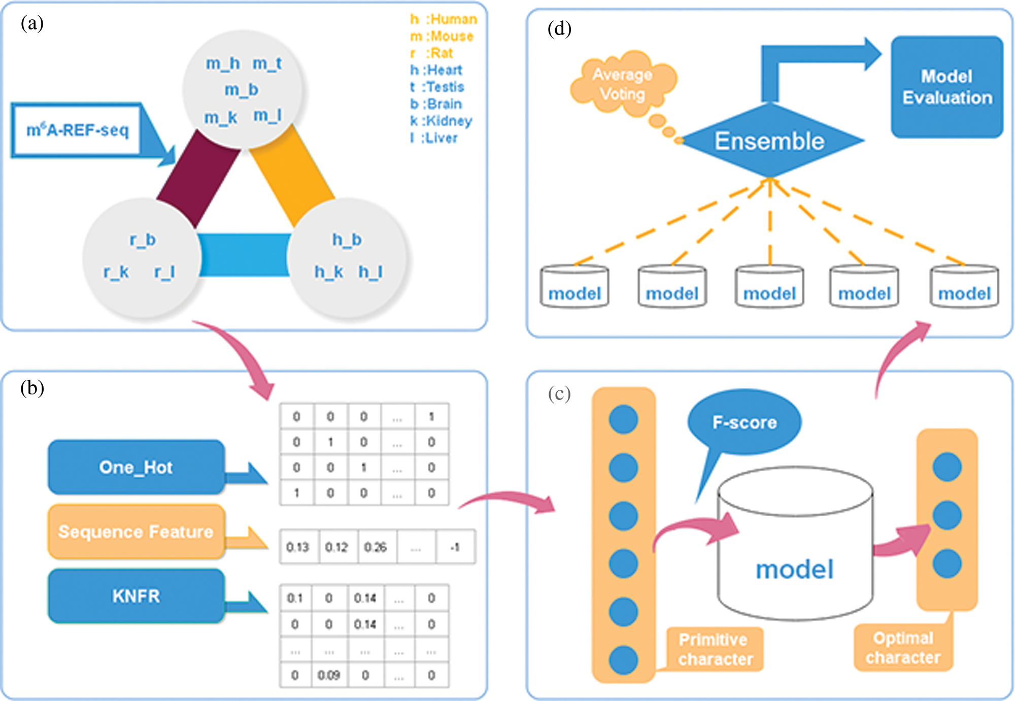
Figure 1: The framework of our model.

Materials and Methods

Datasets

In this study, we trained and evaluated our model on the benchmark datasets containing a total of 11 training and 11 testing datasets from human, mouse and rat, which were also used in iRNA-m6A and im6A-TS-CNN models (Dao et al., 2020; Liu et al., 2020). Each dataset contains the same number of positive and negative samples. Each sample is a 41nt-length RNA sequence with Adenine in the center. Detailed information about these datasets can be found in the work of Dao et al. (2020).

Feature extraction and feature selection

It is vital to extract efficacious features when developing new computational model based on machine or deep learning algorithms (Zhang and Liu, 2019). In this study, we extracted three categories of features from the sequence: one-hot encoding, sequence features, and order features.

One-hot encoding

Given a DNA sequence D, its intuitive expression is

D=R1R2R3R4R5R6R7⋯RL (1)

where RI represents the i -th nucleic acid residue at position i in the DNA sequence.

Each sequence with 41 nt is represented with a 41 × 41 vector, in which (1, 0, 0, 0) stands for G, (0, 1, 0, 0) stands for C, (0, 0, 1, 0) stands for U, and (0, 0, 0, 1) stands for A.

Sequence features

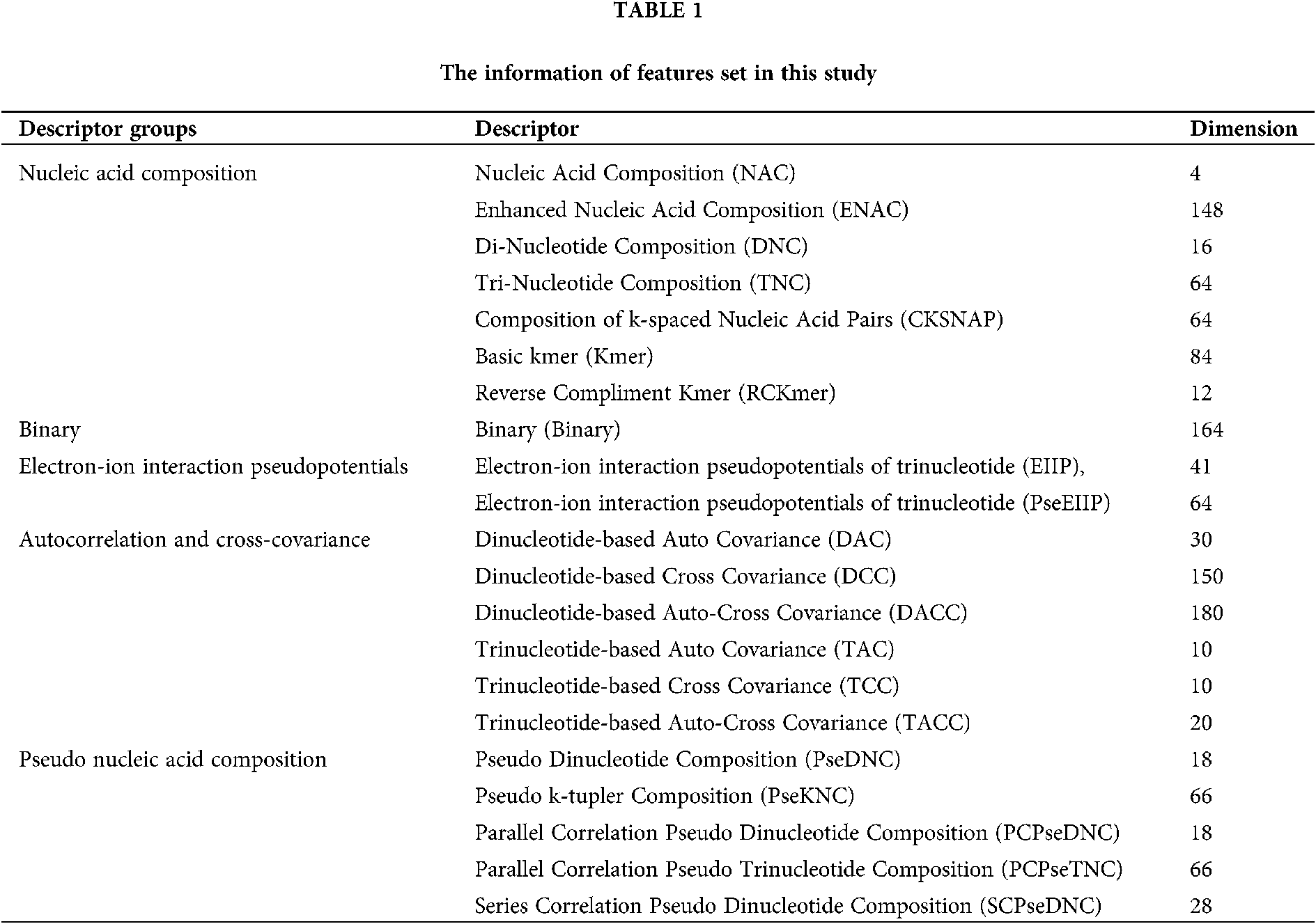
Transforming a DNA sequence sample into a vector based on its sequence characteristic composition is a simple but universal strategy, which can capture significant biological information (Zhen et al., 2020; Zou et al., 2019). iLearn is a comprehensive and versatile Python-based toolkit including a variety of descriptors for DNA, RNA and proteins (Zhen et al., 2020). We used iLearn to calculate and extract four types of features: nucleic acid composition, binary electron-ion interaction pseudopotentials, autocorrelation and cross-covariance, pseudo nucleic acid composition, and achieved a total of 1325 features. The names and dimensions of features used in this section are listed in Table 1. As for the specific definitions of these features, please refer to (Zhen et al., 2020; Zou et al., 2019).

K-tuple nucleotide frequency pattern

KNFP integrates the information from K-mer as well as one-hot encoding, and can compensate for insufficient short-range or local sequence order information effectively (Yang et al., 2020). It has been used to identify protein-RNA binding sites and protein-circRNA interaction sites (Yang et al., 2020). K-mer can map any DNA sequence to a vector with 4k dimensions as follows:

R=[φ1φ2⋯φu⋯φ4k]T (2)

where φu(u=1,2,⋯,4k) is the frequency of the u-th k-mer along the sequence (k = 1,2,3 in this work).

On one hand, R can be transformed to a diagonal matrix RD, if multiplied by the identity matrix. On the other hand, for a DNA sequence D of length L, the number of k-mer is L − k + 1. Each k-mer can be encoded as a one-hot vector with dimension of 4k . The product of the (L−k+1)∗4k matrix (M) and RD is KNFP.

For example, given a sequence S = ‘ACGACGAA’, 1-mer is encoded as one-hot vectors: G = (1, 0, 0, 0), C = (0, 1, 0, 0), U = (0, 0, 1, 0), and A = (0, 0, 0, 1). Then according to the position information, S can be transformed to a matrix as follows:

For S, the frequency vector of 1-mer (G, C, U, A) is R = (0.25, 0.25, 0, 0.5). Then through multiplying R by an identity matrix, it is converted to a diagonal matrix as follows:

The KNFP =M×RD is given as

Feature optimization

Experiments have shown that excessive feature information can interfere with the performance of classifiers. Therefore, feature selection methods should be applied to find the most informative features for training classifiers and thus reduce the dimensionality of the feature vector. F-score has been extensively applied in bioinformatics because of its effectiveness in balancing accuracy and stability (Bui et al., 2016; Li et al., 2018).

The F-score of the j-th feature is defined as

F−score(j)=(x¯j(+)−x¯j)2+(x¯j(−)−x¯j)21m+−1∑k=1m+(x¯k,j(+)−x¯j(+))2+1m−−1∑k=1m−(x¯k,j(−)−x¯j(−))2, (3)

where x¯j,x¯j(+) and x¯j(−) denote average values of the j-th feature in the combined positive and negative training datasets, the positive datasets, and the negative datasets, respectively. m+ is the total number of positive samples; m− is the total number of negative samples; x¯k,j(+) represents the j-th feature of the k-th positive sample and x¯k,j(−) represents the j-th feature of the k-th negative sample. The higher the F-score is, the more useful the corresponding feature is for the classification.

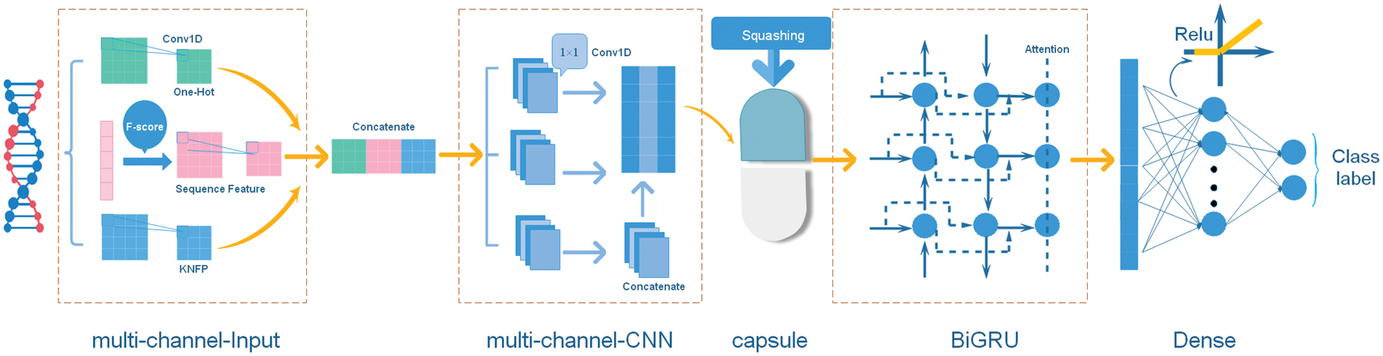
Figure 2: The structure of the multi-input hybrid neural network.

Multi-input hybrid neural network

The model architecture consisted of a multi-channel CNN, a capsule network and a BiGRU network. Each of these three networks has, respectively, been shown to be effective in object detection (Li et al., 2018), protein post-translational modification site prediction (Wang et al., 2019) and social bots detection (Wu et al., 2020). The structure of the multi-input hybrid neural network is shown in Fig. 2.

Multi-channel CNN

The input of the multi-input hybrid neural network is the one-hot encoding, sequence features and KNFP, respectively. For each type of features, we applied 32 convolution filters and performed batch normalization to readjust the data distribution. The input of a batch in the neural network is X=[x1,x2,⋯,xn] , where xi represents a sample and n is the batch size.

The mean value of elements in each batch is obtained by:

μB=1n∑i=1nxi (4)

Then, the variance of a batch is calculated by

σB2=1n∑i=1n(xi−μB)2 (5)

This allows us to normalize each element:

xi′=xi−μBσB2+ϵ (6)

The final output of the network is given by

yi=γi⋅xi′+βi (7)

where ϵ is a small positive number used to prevent the denominator from being 0.

Finally, we merge three outputs using the Swish activation function σ , which is defined as follows:

σ(x)=1/(1+exp⁡(−x)) (8)

Because of the limited size of our datasets, we add a 1 × 1 multi-channel CNN to enhance representational capabilities of the model. The 1 × 1 convolution is used to maintain the size of the feature map and integrate the information by linearly weighting the input feature map of each channel. With additional layers of such 1 × 1 convolution, the final extracted features would become more concise.

Capsule network

The capsule network (CapsNet) was proposed by Sabour et al. (2017) and applied in stance detection (Zhao and Yang, 2020), image recognition (Qian et al., 2020) and automated classification (Mobiny et al., 2019). Since the capsule network collects location information, it can learn a good representation from a small amount of data. We use the capsule network and focus on the hierarchical relationship of local features. The output of the multi-channel CNN is adopted as the input vector of the capsule network. We make an affine transformation of the input vector as follows:

u^j|i=Wijui, (9)

where Wij is the weight matrix that needs to be trained and uI is the input vector of the capsule neural network.

Next, the weighted sum is applied to all the prediction vectors as follows:

sj=∑iciju^j|i, (10)

where cij is the coupling coefficient in the dynamic routing process.

Finally, we obtain output vectors through a non-linear activation function as follows:

vj=‖sj‖21+‖sj‖2sj‖sj‖. (11)

BiGRU network

The third segment of this model is the BiGRU network, which helps to extract deep-level features of sequences. The current hidden layer state of the BiGRU is determined by three factors: the current input xt , the output of the forward hidden layer state at time-step (t–1) ht−1→ and the output of the reverse hidden layer state ht−1← . BiGRU can be regarded as two GRUs, so the state of hidden layer ht at time-step t can be obtained by the weighted sum of the forward hidden layer state ht−1→ and reverse hidden layer state ht−1← :

ht→=GRU(xt,ht−1→) (12)

ht→= GRU(xt,ht−1←) (13)

ht=wt⋅ht→+vt⋅h←t+bt, (14)

where GRU () represents a nonlinear transformation of the input word vector; wt and vt are the weighed matrices; and bt is the bias term.

Parameter setting

Considering the number of datasets and the precision of the model, three feature maps were obtained from batch normalization and 1D convolution with 32 filters (kernel size = 3). The multi-channel CNN contained three 1 × 1 convolution layers and took the Swish as activation function. Considering time cost, we only employed one capsule layer with 14 num_capsule (dim_capsule = 41, routings = 3). The BiGRU had 32 hidden units followed by a fully connected layer and used the ReLU activation function. We also used dropout with a keep probability of 0.3 to prevent the model from over fitting. For stochastic gradient descent, we selected the Adam optimization algorithm. The entire program was written in Python 3.6.

Performance assessment

To evaluate the performance of our prediction model, we used four measurements including accuracy (Acc), sensitivity (Sn), specificity (Sp), and Matthew’s correlation coefficient (MCC) on 5-fold cross-validation and independent dataset tests. The formulas are provided as follows:

{Sp=TNTN+FPSn=TPFN+TPAcc=TP+TNTP+TN+FN+TPMCC=TP×TN−FP×FN(TP+FN)(FP+TN)(TP+FP)(FN+TN) (15)

where TP, TN, FP, and FN represent the number of true positives, true negatives, false positives, and false negatives, respectively.

Results

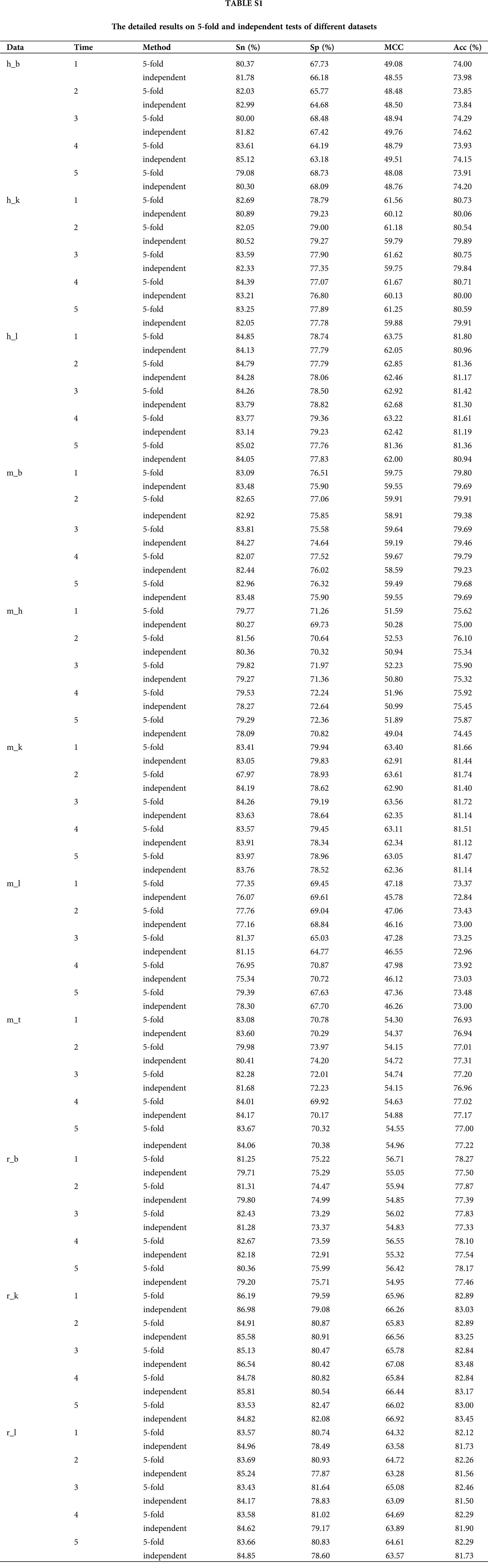
We observed a deviation in the process of 5-fold cross-validation test (Table S1), probably due to the limited number of experimentally verified samples. A general strategy to solve the problem of insufficient samples is to construct an ensemble prediction model. On this purpose, we randomly divided the positive and negative training datasets into five mutually exclusive parts of similar size. And then, we selected the combination of four parts as a new training dataset, while the remaining one part was adopted as validation test dataset to train and optimize the three-layer hybrid neural network at each time. Thus, we got five sub models which were then integrated into a novel ensemble prediction model based on a majority voting strategy.

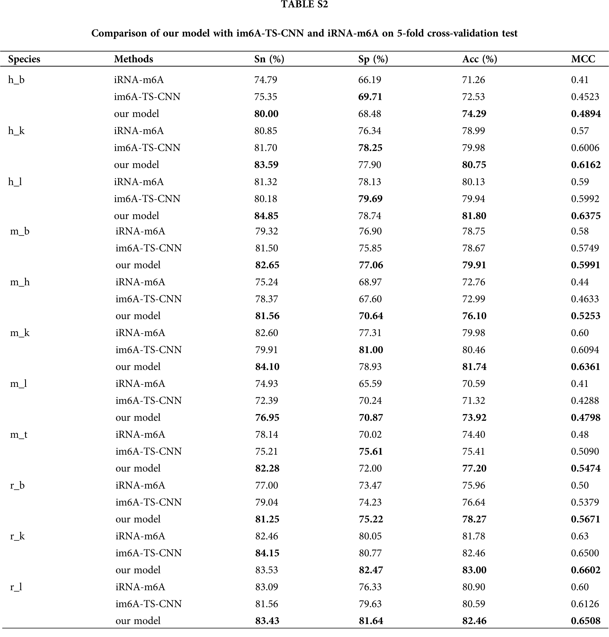
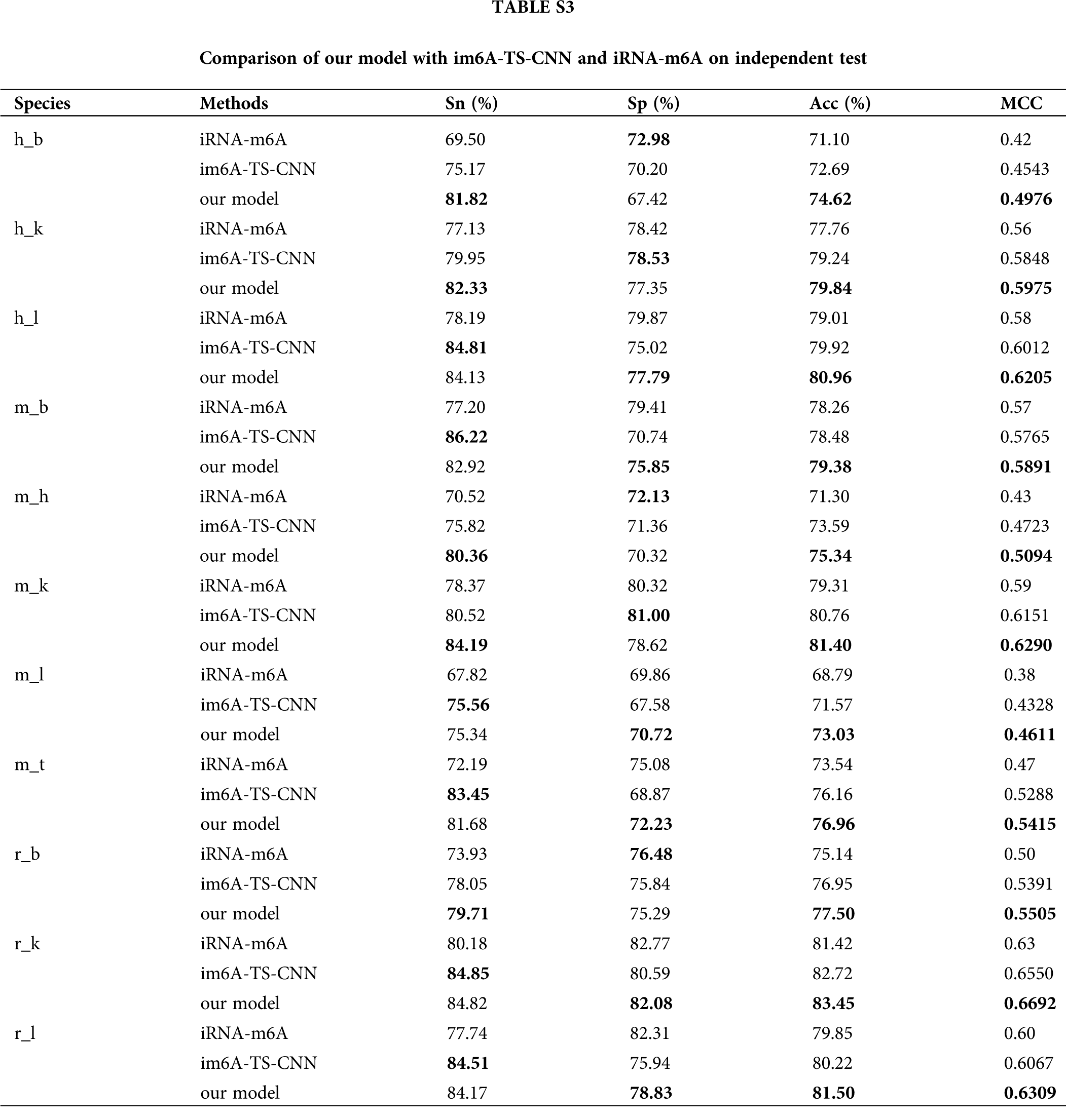
In order to verify the effectiveness of the ensemble model, we compared it with two previous prediction methods: im6A-TS-CNN and iRNA-m6A. The same training and independent datasets were used for our model, im6A-TS-CNN and iRNA-m6A; therefore, both 5-fold cross-validation and independent test could be used to evaluate these methods objectively. There was a total of 132 results from 11 datasets involving four indicators (Sn, Sp, Acc, MCC), among which our model achieved superior predictive performance as measured by average MCC and Acc. Specifically, on the 5-fold cross validation, for Homo sapiens, our model gave MCC = 0.581, vs. 0.550 for the second-placed im6A-TS-CNN; for Musmusculus, our model gave MCC = 0.558 vs. 0.517 for the second-placed im6A-TS-CNN; for Rattusnorvegicus, our model reached MCC = 0.626 vs. 0.600 for the second-placed im6A-TS-CNN. On the independent dataset, for Homo sapiens, our model showed MCC = 0.572 vs. 0.547 for the second-placed im6A-TS-CNN; for Musmusculus, our model gave MCC = 0.546 vs. 0.525 for the second-placed im6A-TS-CNN; for Rattusnorvegicus, our model reached MCC = 0.617 vs. 0.604 for the second-placed im6A-TS-CNN.

To observe the comparison results intuitively, we showed MCC values of these three models in Figs. 3 and 4. Moreover, the comparison results measured with other indicators are provided in Tables S2 and S3.

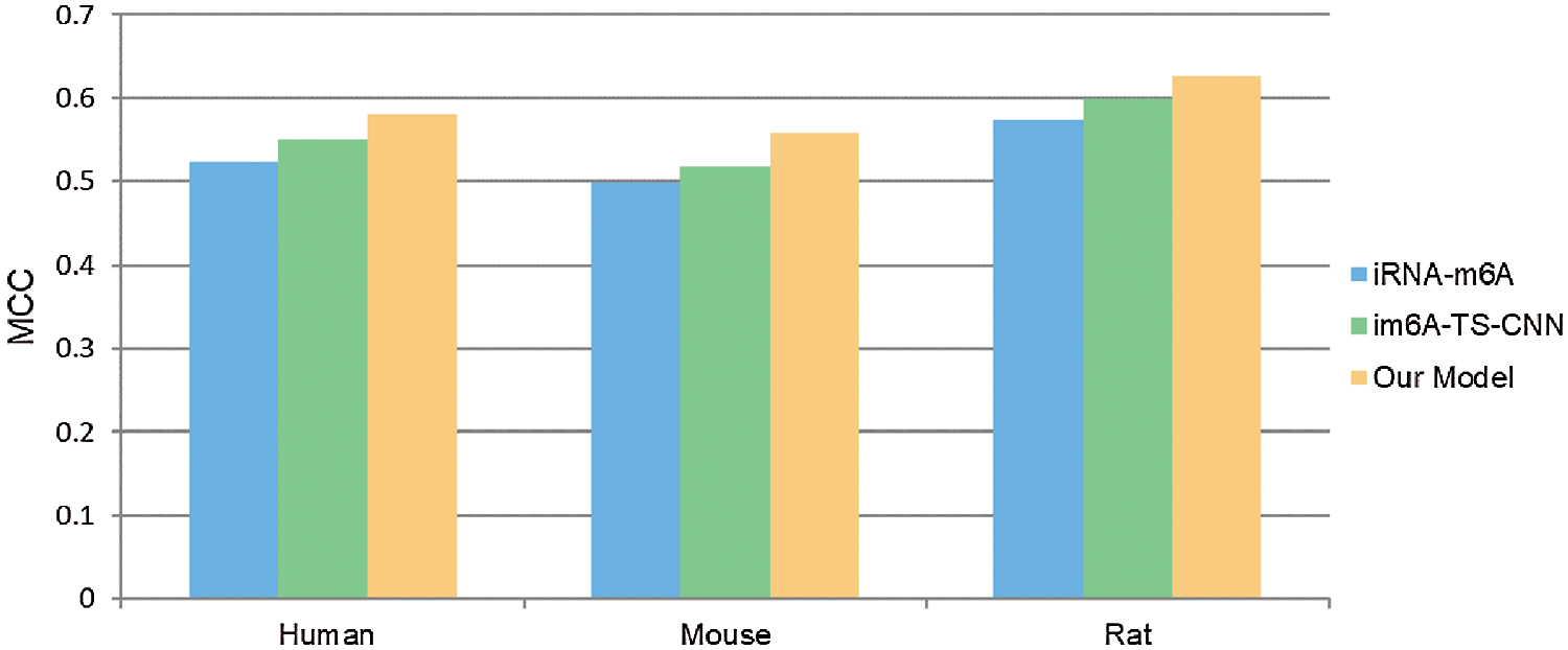
Figure 3: Comparison with MCC measure of different models on 5-fold cross validation test.

Figure 4: Comparison with MCC measure of different models on independent tests.

Discussion

Effectiveness of feature selection

If too many features are extracted, the generalizability of the model will be weakened. Thus it is important to determine the appropriate step size for feature selection. As the dimension of the input matrix was 41 × N, we chose the step size as 41 and evaluated the performance of our model with feature matrices of different dimensions (41 × N, N∈(5,6,7,⋯,24,25) ) on 5-fold cross-validation tests successively. To reduce the deviation caused by the fluctuation of the neural network, we ran each test three times for the 11 datasets from the brain, liver, kidney, heart, and testis of Homo sapiens, Musmusculus, and Rattusnorvegicus. The optimal feature subset was finalized according to the average accuracy. The detailed feature selection results are shown in Fig. 5. As should be noticed, dimensions of optimal features were various for different datasets; their corresponding dimensions are listed in Table 2. These results indicate that it is necessary to establish a specialized model for each tissue type in each species.

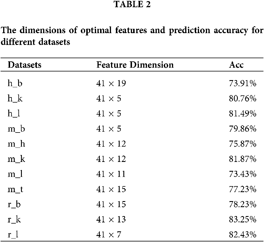
Figure 5: The accuracy comparison of different feature dimension on 11 datasets of three species.

Parameter selection

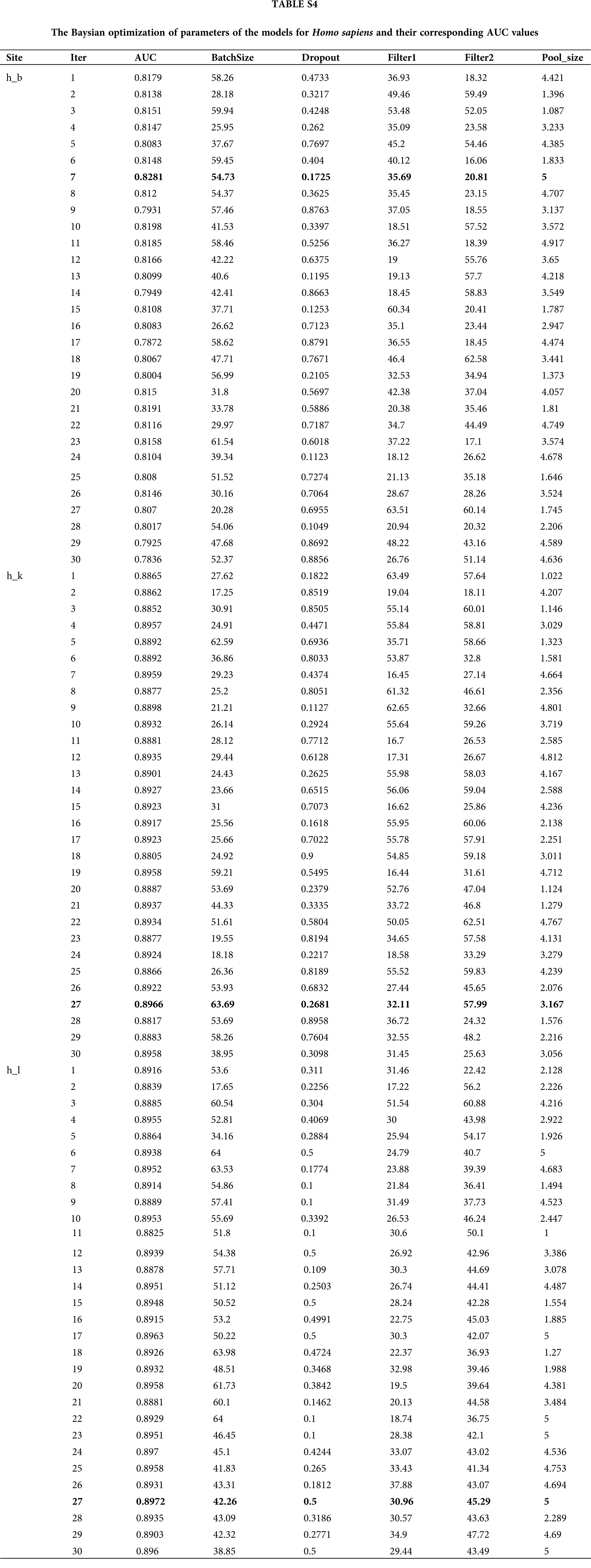
Generally, there are two ways to select parameters, i.e., empirical choice and Bayesian optimization. With Homo sapiens as an example, we tried both methods to find the most suitable parameters. The initial parameters were set based on a previous work to compare the prediction results roughly. Then, if the prediction model was under fitting, we attempted to add more convolution kernels and neurons; otherwise if the prediction model was over fitting, we attempted to reduce the number of convolution kernels and neurons. In addition, batch normalization, dropout, and regularization were introduced to avoid over fitting during the optimizing process. Alternatively, Bayesian optimization (Snoek et al., 2012) was used to tune the key parameters including batch size, dropout rate, filter1, filter2, pool_size and etc. Finally, the optimal parameters wereselected according to the AUC value. The Baysian optimization of parameters in models for Homo sapiens and corresponding AUC values are provided in Table S4 and Fig. 6A. We compared the best results obtained by the two methods and concluded the result given by empirical adjustment parameters showed more advantages (Fig. 6B). Thus, for Musmusculus and Rattusnorvegicus, we used the empirical method to determine the parameters in neural network.

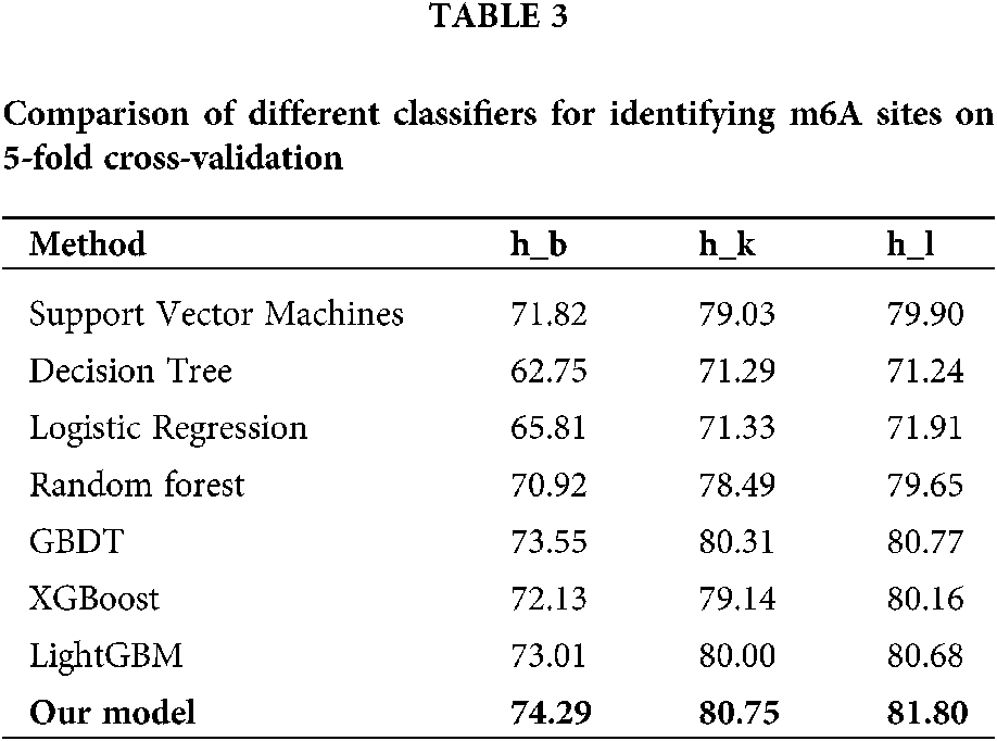
Comparison of different classifiers

To verify the effectiveness of hybrid neural network, we compared its prediction performance with several traditional classification algorithms including logistic regression, decision tree, support vector machine (SVM), random forest (RF), gradient boosting decision tree (GBDT), extreme gradient boosting (XGBoost) and light gradient boosting machine (LightGBM) for Homo sapiens. The average accuracies of 5-fold cross-validation tests obtained by the seven algorithms are listed in Table 3. On three datasets of Homo sapiens, our model achieves the mean accuracy of 74.29%, 1.28% higher than the second best algorithm, LightGBM, which demonstrates that hybrid neural network is capable of improving the recognition performance for m6A sites of various tissues in different species.

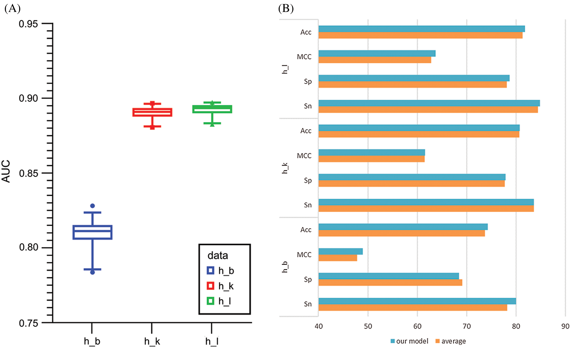
Figure 6: (A) Boxplot comparison results among the Baysian optimization of parameters of the models for Homo sapiens measurements. (B) The comparison results of empirical choice and Bayesian optimization. (C) The t-SNE comparison of different stage for brain tissue.

Visualization of feature representations

To observe the effectiveness of extracted features intuitively, we applied t-distributed stochastic neighbor embedding (t-SNE) to visualize the feature representations. We took the brain tissue as an example and demonstrated the features after mapped through the concatenate layer and the attention layer. Each dot in Fig. 6C represents a sample, with purple dots representing m6A sites and yellow dots representing non-m6A sites. The overlapping of the two sample types on the left side of Fig. 6C indicates that it is difficult to distinguish m6A sites from non-m6A sites. However, the features were relatively separated, as shown on the right side of Fig. 6C, after selected and processed by the deep hierarchical network, which was, multi-channel CNN, capsule network and BiGRU network with the self-attention mechanism. The t-SNE plots indicated that the hybrid deep hierarchical networks could learn sequence motif information from selected features. But there are still some overlaps between the two types, indicating that our model is not completely specific for all m6A sites. This fact is consistent with the need to establish specialized models for each tissue type.

Conclusion

In this work, we introduced a novel ensemble computational approach to identify m6A sites, based on three hybrid neural networks. For different tissues of different species, we selected different optimized feature subsets from 4933 features as multi-input for the deep hybrid neural networks. Our predication model consisted of a multi-channel CNN, a capsule network and a BiGRU network with the self-attention mechanism, and was evaluated on 11 datasets. To solve the deviation caused by the relatively small number of experimentally verified samples, we constructed an ensemble model through integrating five sub-classifiers based on different training datasets. To estimate the performance of this model, comparisons were made on 11 datasets by 5-fold cross validation and independent test datasets. Results of all tests revealed that when measured with Acc and MCC, our model is superior to two previous tools, iRNA-m6A and im6A-TS-CNN. However, the specificity of our model is not satisfactory on h_b, h_k, m_h, m_k and r_b datasets. In future work, we will extract more types of information and further optimize these models.

Availability of Data and Materials: The data sets and source code used in this study are freely available at https://github.com/Dong7777/im6A.

Author Contribution: QZ and XW conceived the project, developed the prediction method, designed and implemented the experiments, analyzed the results, and wrote the paper. DJ and CZJ implemented the experiments, analyzed the results, and wrote the paper. All authors read and approved the final manuscript.

Funding Statement: This work was supported by the National Natural Science Foundation of China (Nos. 62071079 and 61803065).

Conflicts of Interest: The authors declare that they have no conflicts of interest to report regarding the present study.

References

Basith S, Manavalan B, Shin TH, Lee G (2019). SDM6A: A web-based integrative machine-learning framework for predicting 6mA sites in the rice genome. Molecular Therapy Nucleic Acids 18: 131–141. DOI 10.1016/j.omtn.2019.08.011. [Google Scholar] [CrossRef]

Bui VM, Weng SL, Lu CT, Chang TH, Weng JT, Lee TY (2016). SOHSite: Incorporating evolutionary information and physicochemical properties to identify protein S-sulfenylation sites. BMC Genomics 17: 1–9. DOI 10.1186/s12864-015-2299-1. [Google Scholar] [CrossRef]

Cao G, Li HB, Yin Z, Flavell RA (2016). Recent advances in dynamic m6A RNA modification. Open Biology 6: 160003. DOI 10.1098/rsob.160003. [Google Scholar] [CrossRef]

Chen W, Feng P, Yang H, Ding H, Lin H, Chou KC (2018). iRNA-3typeA: Identifying three types of modification at RNA’s adenosine sites, molecular therapy. Molecular Therapy Nucleic Acids 11: 468–474. DOI 10.1016/j.omtn.2018.03.012. [Google Scholar] [CrossRef]

Chen W, Xing P, Zou Q (2017). Detecting N6-methyladenosine sites from RNA transcriptomes using ensemble support vector machines. Scientific Reports 7: 40242. DOI 10.1038/srep40242. [Google Scholar] [CrossRef]

Dao FY, Lv H, Yang YH, Zulfiqar H, Lin H (2020). Computational identification of N6-methyladenosine sites in multiple tissues of mammals. Computational and Structural Biotechnology Journal 18: 1084–1091. DOI 10.1016/j.csbj.2020.04.015. [Google Scholar] [CrossRef]

Feng P, Yang H, Ding H, Lin H, Chen W et al. (2019). iDNA6mA-PseKNC: Identifying DNA n6-methyladenosine sites by incorporating nucleotide physicochemical properties into PseKNC. Genomics 111: 96–102. DOI 10.1016/j.ygeno.2018.01.005. [Google Scholar] [CrossRef]

Hasan MM, Manavalan B, Shoombuatong W, Khatun MS, Kurata H (2020). i6mA-Fuse: Improved and robust prediction of DNA 6mA sites in the Rosaceae genome by fusing multiple feature representation. Plant Molecular Biology 103: 225–234. DOI 10.1007/s11103-020-00988-y. [Google Scholar] [CrossRef]

Li QX, Rong CH, Cai YX, Ran S, Yi WL (2018). M6AMRFS: Robust prediction of N6-methyladenosine sites with sequence-based features in multiple species. Frontiers in Genetics 9: 495. DOI 10.3389/fgene.2018.00495. [Google Scholar]

Liu K, Cao L, Du P, Chen W (2020). im6A-TS-CNN: Identifying the N(6)-methyladenine site in multiple tissues by using the convolutional neural network. Molecular Therapy Nucleic Acids 21: 1044–1049. DOI 10.1016/j.omtn.2020.07.034. [Google Scholar] [CrossRef]

Liu S, Liu Z (2017). Multi-channel CNN-based object detection for enhanced situation awareness. Sensors and Electronics Technology (SET) Panel Symposium SET-241 on 9th NATO Military Sensing Symposium. [Google Scholar]

Liu Z, Xiao X, Yu DJ, Jia J, Qiu WR, Chou KC (2016). pRNAm-PC: Predicting N(6)-methyladenosine sites in RNA sequences via physical-chemical properties. Analytical Biochemistry 497: 60–67. DOI 10.1016/j.ab.2015.12.017. [Google Scholar] [CrossRef]

Mobiny A, Lu H, Nguyen HV, Roysam B, Varadarajan N (2019). Automated classification of apoptosis in phase contrast microscopy using capsule network. IEEE Transactions on Medical Imaging 39: 1–10. DOI 10.1109/TMI.2019.2918181. [Google Scholar] [CrossRef]

Nazari I, Tahir M, Tayara H, Chong KT (2019). iN6-methyl (5-stepIdentifying RNA N6-methyladenosine sites using deep learning mode via chou’s 5-step rules and chou’s general PseKNC. Chemometrics and Intelligent Laboratory Systems 193: 103811. DOI 10.1016/j.chemolab.2019.103811. [Google Scholar] [CrossRef]

Qi CK, Zhen W, Qing Z, Yu WX, Rong R, Liang LZ, Long SJ, João MP, Daniel JR, Jia M (2019). WHISTLE: A high-accuracy map of the human N6-methyladenosine (m6A) epitranscriptome predicted using a machine learning approach. Nucleic Acids Research 47: e41. DOI 10.1093/nar/gkz074. [Google Scholar] [CrossRef]

Qian K, Tian L, Liu Y, Wen X, Bao J (2020). Image robust recognition based on feature-entropy-oriented differential fusion capsule network. Applied Intelligence 51: 1108–1117. DOI 10.1007/s10489-020-01873-3. [Google Scholar]

Sabour S, Frosst N, Hinton GE (2017). Dynamic routing between capsules. 31st Conference on Neural Information Processing Systems (NIPS 2017), Long Beach, CA, USA. [Google Scholar]

Shahid A, Maqsood H (2018). iMethyl-STTNC: Identification of N 6-methyladenosine sites by extending the idea of SAAC into Chou’s PseAAC to formulate RNA sequences. Journal of Theoretical Biology 455: 205–211. DOI 10.1016/j.jtbi.2018.07.018. [Google Scholar] [CrossRef]

Snoek J, Larochelle H, Adams RP (2012). Practical Bayesian optimization of machine learning algorithms. In: Advances in Neural Information Processing Systems, vol. 4. [Google Scholar]

Tahir M, Tayara H, Chong KT (2019). iDNA6mA (5-step ruleIdentification of DNA N6-methyladenine sites in the rice genome by intelligent computational model via chou’s 5-step rule. Chemometrics & Intelligent Laboratory Systems 189: 96–101. DOI 10.1016/j.chemolab.2019.04.007. [Google Scholar] [CrossRef]

Wang D, Liang Y, Xu D (2019). Capsule network for protein post-translational modification site prediction. Bioinformatics 35: 2386–2394. DOI 10.1093/bioinformatics/bty977. [Google Scholar] [CrossRef]

Wei L, Chen H, Ran S (2018). M6APred-EL: A sequence-based predictor for identifying N6-methyladenosine sites using ensemble learning. Molecular Therapy Nucleic Acids 12: 635–644. DOI 10.1016/j.omtn.2018.07.004. [Google Scholar] [CrossRef]

Wei C, Hua T, Hao L (2016). MethyRNA: A web-server for identification of N(6)-methyladenosine sites. Journal of Biomolecular Structure & Dynamics 35: 1–11. DOI 10.1080/07391102.2016.1157761. [Google Scholar] [CrossRef]

Wu Y, Fang Y, Shang S, Jin J, Wang H (2020). A novel framework for detecting social bots with deep neural networks and active learning. Knowledge-Based Systems 211: 106525. DOI 10.1016/j.knosys.2020.106525. [Google Scholar] [CrossRef]

Xing P, Su R, Guo F, Wei L (2017). Identifying N6-methyladenosine sites using multi-interval nucleotide pair position specificity and support vector machine. Scientific Reports 7: 46757. DOI 10.1038/srep46757. [Google Scholar] [CrossRef]

Yan AC, Liang Y, Quan Z (2021). Prediction of bio-sequence modifications and the associations with diseases. Briefings in Functional Genomics 20: 1–18. DOI 10.1093/bfgp/elaa023. [Google Scholar]

Yang C, Hu Y, Zhou B, Bo Z, Lu BY, Bin LZ, Li GC, Huan Y, Min WS, Feng XY (2020). The role of m6A modification in physiology and disease. Cell Death & Disease 11: 960. DOI 10.1038/s41419-020-03143-z. [Google Scholar] [CrossRef]

Zhang J, Liu B (2019). A review on the recent developments of sequence-based protein feature extraction methods. Current Bioinformatics 14: 190–199. DOI 10.2174/1574893614666181212102749. [Google Scholar] [CrossRef]

Zhao G, Yang P (2020). Pretrained embeddings for stance detection with hierarchical capsule network on social media. ACM Transactions on Information Systems 39: 1. DOI 10.1145/3412362. [Google Scholar] [CrossRef]

Zhao X, Zhang Y, Ning Q, Zhang H, Ji J, Yin M (2019). Identifying N6-methyladenosine sites using extreme gradient boosting system optimized by particle swarm optimizer. Journal of Theoretical Biology 467: 39–47. DOI 10.1016/j.jtbi.2019.01.035. [Google Scholar] [CrossRef]

Zhen C, Pei Z, Yi LF, Tatiana TM, André L et al. (2020). iLearn: An integrated platform and meta-learner for feature engineering, machine-learning analysis and modeling of DNA, RNA and protein sequence data. Briefings in Bioinformatics 21: 1047–1057. DOI 10.1093/bib/bbz041. [Google Scholar] [CrossRef]

Zou Q, Xing P, Wei L, Liu B (2019). Gene2vec: Gene subsequence embedding for prediction of mammalian N6-methyladenosine sites from mRNA. RNA 25: 205–218. DOI 10.1261/rna.069112.118. [Google Scholar] [CrossRef]

Supplementary Tables

This work is licensed under a Creative Commons Attribution 4.0 International License, which permits unrestricted use, distribution, and reproduction in any medium, provided the original work is properly cited.