DOI:10.32604/cmc.2020.013125
| Computers, Materials & Continua DOI:10.32604/cmc.2020.013125 | |
| Article |
Detecting Lumbar Implant and Diagnosing Scoliosis from Vietnamese X-Ray Imaging Using the Pre-Trained API Models and Transfer Learning
1Duy Tan University, Da Nang, 550000, Vietnam
2Department of Radiology, Hue University of Medicine and Pharmacy, Hue University, Hue, 530000, Vietnam
3Institute of Research and Development, Duy Tan University, Danang, 550000, Vietnam
4Faculty of Information Technology, Duy Tan University, Danang, 550000, Vietnam
*Corresponding Author: Dac-Nhuong Le. Email: ledacnhuong@duytan.edu.vn
Received: 27 July 2020; Accepted: 11 September 2020
Abstract: With the rapid growth of the autonomous system, deep learning has become integral parts to enumerate applications especially in the case of healthcare systems. Human body vertebrae are the longest and complex parts of the human body. There are numerous kinds of conditions such as scoliosis, vertebra degeneration, and vertebrate disc spacing that are related to the human body vertebrae or spine or backbone. Early detection of these problems is very important otherwise patients will suffer from a disease for a lifetime. In this proposed system, we developed an autonomous system that detects lumbar implants and diagnoses scoliosis from the modified Vietnamese x-ray imaging. We applied two different approaches including pre-trained APIs and transfer learning with their pre-trained models due to the unavailability of sufficient x-ray medical imaging. The results show that transfer learning is suitable for the modified Vietnamese x-ray imaging data as compared to the pre-trained API models. Moreover, we also explored and analyzed four transfer learning models and two pre-trained API models with our datasets in terms of accuracy, sensitivity, and specificity.
Keywords: Lumbar implant; diagnosing scoliosis; X-Ray imaging; transfer learning
Lower back pain is one of the most common illnesses all over the world and is a leading cause of morbidity as well as an increasing burden on global health care [1,2]. Recognizing the particular etiology is a hurdle for the health system, although the causes of pain are usually due to mechanical pressing or chemical irritation that leads to nervous inflammation [3]. The main causes of the low back are spinal stenosis and disc herniation [4]. Intervertebral disks have complex and unique structure is very complex and unique [5]. The intervertebral disk supports load transfer across the vertebrae due to the highly mobile nature of the spinal columns. From the biomedical point of view, joints in the intervertebral disk have dynamic properties such as changing nature. These properties are changed as per human life and age. However, the degeneration of the disk in the human body can be slowed down [6–8]. The lower region in the spine called the lumbar spine is a highly affected area in disk degeneration. This lead [9] to chronic pain in the back. The pain gets worse at the time of movement of the spine. Generally, this disease leads to altered social relations [10] due to related medication and disability especially in the case of the working people. Particular treatment cost [11] of the spine is mainly on the medical imaging from the initial diagnosis to surgical treatment pathway. To diagnose a spine disease, there are three kinds of imaging techniques used including X-ray, Computer Tomography (CT), and Magnetic Resonance Imaging (MRI). X-rays are the most common and widely used imaging technique. These are the radiations passing through the body and are being absorbed by the human body. However, attenuation of X-Ray is dependent on the thickness and density of the tissues. CT scan and MRI both capture a more detailed medical image of the vertebrae, spine, and other internal body organs. These techniques allow the radiologist to recognize the problem location and etiology [12]. Interpretation of the imaging techniques can be complex and time-consuming especially in cases where multiple degradations are found. There is a lack of universally accepted criteria for image quality which can degrade [13].
To address these limitations, several computer-aided methods have been proposed by many researchers over the past few decades. There are many previous studies done on computer aided techniques such as histogram oriented [14–17] and GrowCut [18,19] to execute the vertebral discs segmentation. Some studies are based on automated spine degenerations, Neubert et al. [20] used the analysis of statistical shapes to extract the three-dimensional model of lumbar in the human body spine. In Peng et al. [21], the author proposed an algorithm that worked on the two phases:
1.Localization of the intervertebral disk,
2.Vertebrae detection, and segmentation.
The model searching method was applied to find the location of all clues in the intervertebral discs. Authors [22] developed an autonomous system that is used to recognize and evaluate the spinal osteophytes on CT studies. They applied a three-tier learning method to calculate the confidence map and identify the osteophytes clusters. To identify the degeneration grading of a single intervertebral spine in MRI scanning was proposed by Lootus et al. [23]. The rapid growth of deep learning solves many problems especially in the case of healthcare diagnosis where the normal computed aided techniques computation power is limited. Undoubtedly, convolutional neural networks (CNN) got appreciation over the global research communities for its learning capability where algorithms can autonomously learn from raw data, perform the multi-layer classification and achieve high accuracy outcomes [24–29]. Suzani et al. [30] presented a deep forward neural network-based automated system to recognize and localize the vertebrae in the CT scan images. Wang et al. [26] developed a system that incorporates three similar subnetworks for a bunch of resolution analyses and recognition of spinal metastasis. With the aid of contextual information, it can predict the location of every vertebra in the human body spine. Pixel series segmentation was applied in the series network and MRI images segmented differently. The output of one network was directly connected to the input of the other proposed by Whitehead et al. [31].
To deal with the huge range of spine problems such as degenerative phenomena as well as coronal deformities, the automated method was discussed by Galbusera et al. [32]. This method is applied to extract the anatomical characteristic from the radiographic images based on a biplane. Some of the researchers were focused on analyzing the lumbar vertebra and applied deep learning models on the X-ray images and the rest of them applied to the CT Scan or MRI images. The Faster R-CNN method was applied for the detection of intervertebral discs in the X-Ray images [33]. 81 images were used in this study with annotated clinical data. Kuok et al. [34] presented a dual method to scrutinize the vertebrae segmentation in the X-Ray Image. In this dual method, the vertebral region was recognized via an image processing technique and then applied to CNN for the vertebrae segmentation. To detect the compression fracture and analysis on lumbar vertebra X-Ray images, integration of deep learning with level-set methods had been proposed by Kim et al. [35]. This study also used the same method: one to identify the vertebra and another one is for the segmentation. Deep learning approaches are mostly applied to the MRI and CT images due to its 360 degrees coverage of the human body part. An autonomous deep learning-based model was proposed to detect, identify and label the spine vertebrae in the MRI images [36–38], and the same in the case of CT images [39–41]. X-ray images and MRI/CT scan images have their own benefits and limitations. Usually, in the healthcare sector, datasets are very limited due to the security and privacy issue in hospitals and care centers. There are some ways to overcome these issues:
1.Combine the datasets of different public repositories with the personal dataset.
2.Apply the transfer learning method on the person dataset.
Zhao et al. [42] introduced a study based on transfer learning for the segmentation and localization of spinal vertebrae (see Tab. 1).
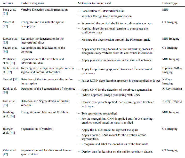
Table 1: Studies related to the diagnosis of human body spine
The integration of transfer learning in deep learning applications moved applications toward a new era of technology especially in the case of medical imaging [43]. The major drawback of the medical imaging system is the lack of private datasets and public repositories are also very limited. Transfer learning is able to overcome these issues through the usage of fine-tuning. Radiologists use X-Ray imaging, MRI imaging, or CT scan imaging to follow the spine problem such as a lumbar implant, scoliosis, and vertebrae degeneration from the early to the most critical stage. Sometimes the quick detection of spine disease in medical imaging is quite complex and analyzing these images can be time-consuming. Thus, there is a pressing demand to build an autonomous detention system for the human body spine. This research provides a state-of-the-art solution to detect the lumbar implant and scoliosis in the Vietnamese X-Ray imaging dataset. Then we build the autonomous detection system using the API Pre-Trained models and transfer learning tools. Moreover, different pertained models in the API and transfer learning are applied to the X-Ray imaging dataset. Then, we analyze the deployed model and selection of the best model which is suitable for the proposed task. From the technical point of view, the major contributions of this paper are as follow:
1.We set up a ready-to-use dataset from X-Ray images. To increase our dataset, added more images from multiple sources to make the proposed system more realistic to detect the lumbar implant and diagnose scoliosis.
2.We also converted MRI spine imaging to DICOM to enhance the dataset.
3.We applied two different approaches to the diagnosis of the Vietnamese X-Ray imaging dataset.
4.Two Pre-Trained models in the first approach and Four Pre-Trained in the second approach to accelerate and elevate the diagnosis power.
The rest of the paper is discussed as follows: Section 2 provides the Model regime for the proposed system. Section 3 discusses the methodology. Section 4 illustrates the workflow of the dataset. Section 5 discusses the result and evaluation of the proposed study. Finally, Section 6 concludes this study.
Training a model is a time-consuming process to achieve the highest level of accuracy and high-performance results [44,45]. It also requires large datasets that are very strenuous to collect especially in the case of healthcare. To overcome these issues, Pre-trained models are a valuable asset. Moreover, it achieves high-performance results in a shorter time as well as does not require a well-labeled dataset. Some of the models used in the proposed system are discussed as follows:
Ren et al. [46] proposed a well-known neural network called Faster-RCNN for object detection. This neural network can also be derived for image segmentation, 3D object detection. With the conceptual point of view, Faster CNN is the combination of three different neural networks such as Detection Network (DN) or Region-based convolutional neural network (RCNN), Region Proposed Network (RPN) as well as Feature Network (FN). FN is a pre-trained network based on image classification such as visual geometry group (VGG) eliminating the top layers/some last layers. The purpose behind this network is to build new features from the input image and manage the shape and structure of the input image that includes pixels, and rectangular dimensions. The RPN is composed of three convolutional layers. There is a single and common layer that is connected to further two layers: 1) Classification 2) Bounding box regression. RPN is used to build a bunch of bounding boxes called Region of Interests (ROI) that show a higher possibility of object detection. The result outcomes from this network are the identification of numerous bounding boxes via pixel coordinates of two lopsided corners. The final layer RCNN or the Detection network gets input from both layers, FN and RPN, and builds the outcome in the form of class and bounding box. This layer is packed up with layers that are fully connected or dense. This technique helps to classify the image inside bounding boxes, the features are trimmed as per the bounding box conditions. The loss function of the network defined as (Eq. (1)):

where, Oi is the predicted probability of anchor i being as the object; Oi* is the ground truth label of whether anchor i an object; ti is the predicted anchor coordinates; ti*:is the coordinates of the ground truth attached with the bounding box; Lcls is the loss in classifier; Lreg is the loss in regression; Ncls is the normalization parameters of mini-batch size; Nreg is the normalization parameter of regression.
Residual Network (ResNet) is the exemplary neural network that works for numerous computer vision applications proposed by He et al. [47]. In 2015, this model won the ImageNet challenge. The ResNet model is permitted to train the 150+ layer on deep neural networks. However, it is difficult to train a very deep neural network because of the vanishing gradient. These barriers are broken with the introduction of ResNet. In 2012, AlexNet won the ImageNet challenges but its ability to train the deep learning model is limited up to 8 convolutional layers and in the case of VGG [48] and GoogleNet [49] has 19 and 22 respectively. The skipping concept is introduced in the ResNet and highlighted in the Kobayashi et al. [50] study (see in Fig. 1).
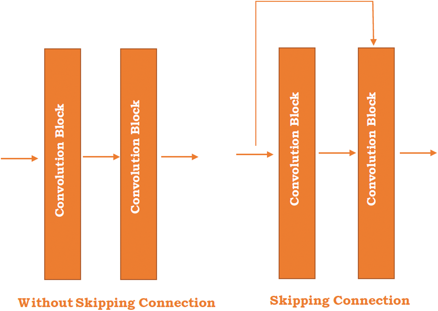
Figure 1: Skipping connection in the ResNet
Fig. 1 illustrates the two different figures where one is without skipping connection and the other is skipping the connection between the two convolutional blocks. The skipping connection refers to the original input image directly passed to the output of the convolutional block and skipped by some convolution block. The right-hand side image shows the skipping connections between the blocks. The main reason behind the skip connection is to diminish the vanishing gradient problem through another shortcut path for the gradient to pass and allow the model for grasping an identity function which sets the seal on higher and lower layer performance will be the same.
Szegedy et al. [51] proposed a study “Going Deeper with convolution” named Inception network. The Inception network is a state of art architecture based on deep learning which is beneficial for resolving the image object detection and recognition obstacles. The purpose of this model is a deep neural network that can sustain the budget of computation while extending the size of the network in terms of depth and width. There are some problems generated while using bigger models such as overfitting and increasing the computational cost of the network. Although, Inception networks can overcome these issues with the replacement of the sparsely connected network to fully connected network architecture. Inceptions are based on the convolutional neural network that is 27 layers deep combined with the inception layers. These layers are the core concept of inception’s sparsely connected networks. “Inception layer is the amalgamation of different convolutional layers with multi-filter banks intended towards single output that creates the next stage input” (see in Fig. 2).
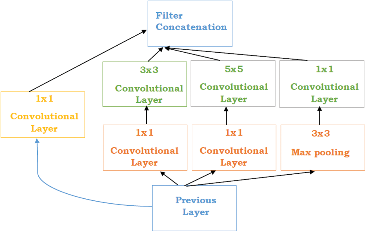
Figure 2: Inception layers [51]
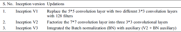
Tab. 2 represents the Inception versions that are extended from the traditional inception version.
Table 2: Inception versions [51]
Iandola et al. [52] proposed a small architecture named SqueezeNet that can achieve the AlexNet accuracy with three times faster and 50x smaller parameters. In the SqueezeNet, 3 × 3 filters are replaced by the 1 × 1 layer which diminishes the depth and computation time. Fire modules are the building bricks of the SqueezeNet that contains two different layers 1) squeeze layer: 1 × 1 filter 2) Expand layer: 1 × 1 and 3 × 3 layer. The Squeeze layer provides feeding to the Expanded layer with 1 × 1 and mixes with the existing layer. The Squeezing network has three different strategies as follow:
•Change 3 × 3 filter with the 1 × 1 filter to reduce the network size.
•With the use of fewer filters, the number of inputs or parameters will reduce.
•Large activation maps in the convolution layers due to the down sample late in the network.
SqueezeNet architecture starts with a convolutional neural network, comes after eight fire modules, and finishes with a final convolutional layer. The number of filters per fire module is gradually expanded from start to finish of the network. Moreover, the squeeze net executes the max-pooling through the stride of two after the convolutional 1, fire 4, 8, and convolutional 10.
Huang et al. [48] proposed a network called DenseNet in 2016 and this network is based on the 0 CNN architectures that achieved highly specific and state of the art results on the popular datasets such as CIFAR, SVHN, and ImageNet for the classification purpose through the use of some parameters. DenseNet is the combination of dense blocks and these blocks are further densely connected to each other. Every layer gets input from all forgoing layers output feature maps. Every layer gets feature maps from all foregoing layers, so the size and dimensions of the network can be small and thinner i.e., input parameters can also be small. So, the network has higher computational and memory efficiency.
DenseNet overcomes some issues as follows:
•DenseNet requires a smaller number of parameters as compared to the traditional CNN and also skips the learning of redundant features maps.
•The layers in the DenseNet are very less as compared to the ResNet and can be updated with a limited number of new feature maps.
•DenseNet sets up a bridge between the layer and gradient from loss function and source image which can solve the model training issues in traditional networks.
A deep DenseNet is combined with the three dense blocks, transition layers, and transition of feature map size through the convolution and pooling. In this study [48] shows that with the increasing number of parameters, accuracy will also improve consistently without any degradation of performance or overfitting.
This section illustrates the design of the usage of pre-trained models and transfers learning to recognize the lumbar implant and diagnosis scoliosis in the vertebrae of the spine. This proposal includes two different approaches: 1) Pre-Trained models API 2) Using Transfer learning with pre-trained models. Due to the medical data limitation, these approaches are highly beneficial to recognize the problems in radiology imaging. Fig. 3 represents the architecture of the proposed work.
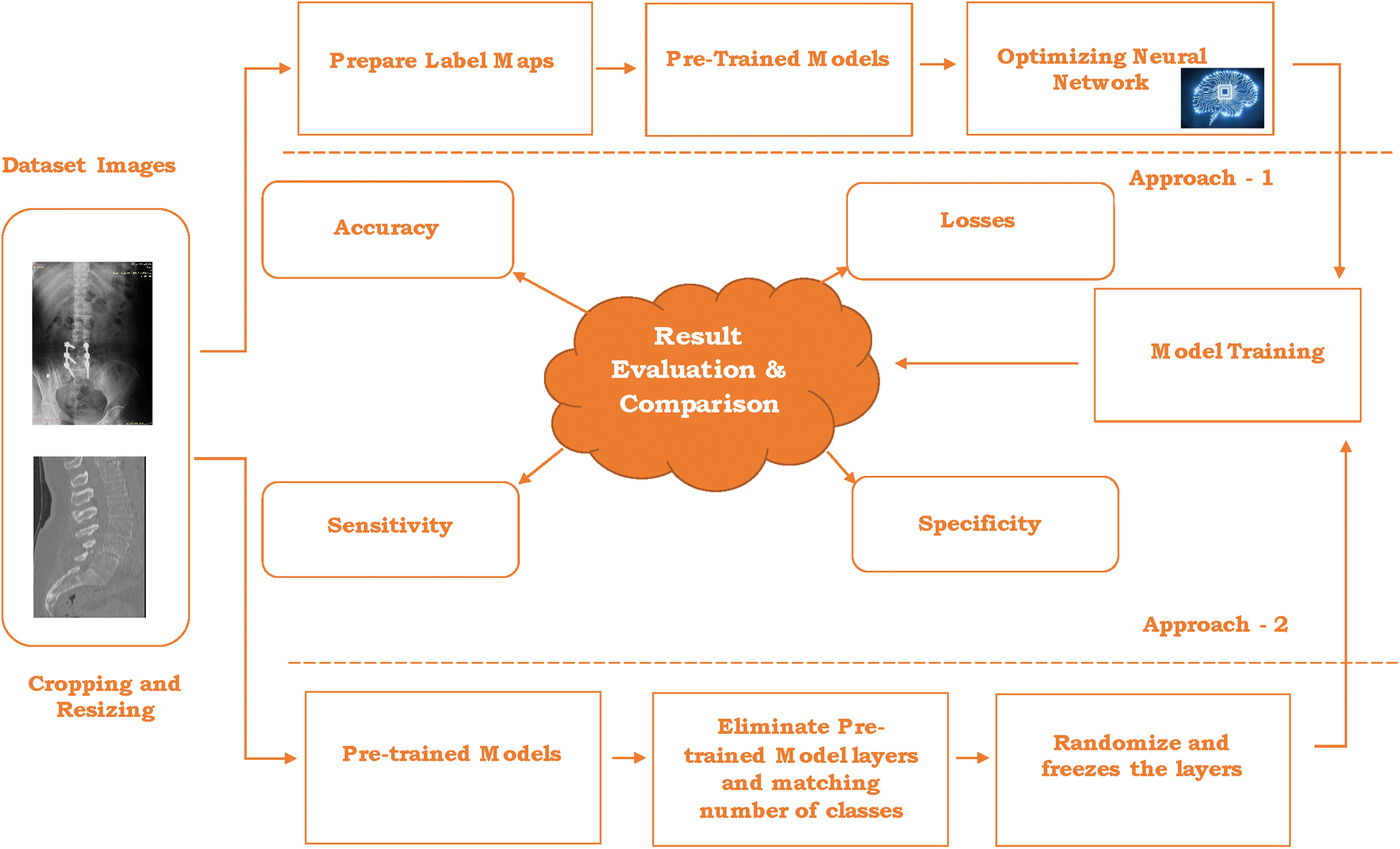
Figure 3: Architecture for the proposed work
The combined dataset (discussed in Section 4) contains many images from different datasets including the Vietnamese x-ray imaging, MRI imaging, and scoliosis imaging. Although the size and dimension of the images used in a combined dataset are different that leads to creating problems at the time of model training and optimizing the network. The first step is to crop and resize the images in the same dimension and particular size. In the proposed work, images are cropped and resized into 48 × 48 pixels for further processing. After cropping and resizing the images, annotation is done. Image annotation is a human-powered task to annotate the image with labels that help to recognize the image at the time of prediction.
In every image, the number of labels varies as per the classification of objects. In this system, Lumbar implant and scoliosis are detected and diagnosis respectively through the two different approaches as follow:
3.1 Approach 1: Pre-Trained Model API’s
In the first attempt, the API method is deployed in the system. API stands for application program interface which provides typical operations to the developer or user for developing AI systems without doing any harsh coding from scratch. TensorFlow API [53,54] is the framework based on deep learning which helps to overcome the object detection issues and make an object detection model easy to develop, train, and test. In the TensorFlow API system already has some pre-trained models such as faster_rcnn_resnet50_coco, faster_rcnn_inception_v2_coco, ssd_mobilenet_v2_coco, and many more [55]. These models are further based on some big dataset models such as COCO trained model, mobile model, Pixel edge TPU model, KITI trained model, and open-image dataset models. These models are like “Out-of-Box” for those object detection systems where objects are matched with a pre-trained model dataset. However, our system is based on detecting the lumbar implant and diagnosis scoliosis x-ray imaging that is different from the pre-trained datasets models. In this case, we need to modify the pre-trained dataset as per the need and the steps for the system as follows:
TensorFlow object detection API requires label maps that means every label used in the system has integer values. These values used in the label maps are required at the time of model training as well as the detection process (see Fig. 4).
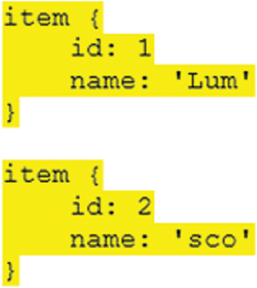
Figure 4: Label maps format for the proposed syst
Two different labels are employed in our system and label names and id’s for the lumbar implant and scoliosis are “Lum”, “1” and “sco”, “2” respectively. The next step is to convert and store dataset images and their annotation files in the sequence of the binary records and save the train and test images with record extensions that are used for further processing.
3.1.2 Pretrained Models and Optimizing Neural Network
In the TensorFlow object detection API, there are some models with different datasets available. Faster_rcnn_inception_v2_coco and faster_rcnn_inception_resnet_v2_atrous_oidv2 are pre-trained models based on Faster CNN with Inception and Faster RCNN with Inception and ResNet respectively. It is also based on two different datasets, COCO and Open-Trained Images models are respectively considered in this study to recognize scoliosis and lumbar implants in X-ray imaging. Before training, we need to configure these models with the proposed dataset. The configurations of the models are discussed in Tab. 3.
Table 3: Configuration setting in the pre-trained models
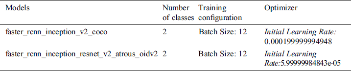
In both models, configuration for the class and training are the same but network optimizing learning rate is different in both cases.
After the configuration of pre-trained models with the medical imaging data, the dataset is ready to train. Processing time varies as per the selected batch size and system GPU. Larger batch size means processing time will be high. The total loss parameter is the way to monitor the performance of training models. We need to monitor the total loss value until lower values are not achieved. But very low value means the model will end up with overfitting which means object detection will work poorly. So, it is mandatory to select the fair value for the object detection system.
3.2 Approach 2: Transfer Learning
The second approach in the proposed study is Transfer learning. With the growth in the deep learning applications, transfer learning is integrated into numerous applications especially in the case of medical imaging. Four pre-trained networks include ResNet, SqueezeNet, InceptionV3, and DenseNet belong to convolution neural network family which has trained a million images with thousand classes on the ImageNet [56]. The main motive behind using the pre-trained network is to transfer bias, weight, and features to the imaging dataset for the prediction of lumbar implant and scoliosis. Compared to Transfer learning, the CNN network takes more time and computational power due to initializing random weight from the beginning. Transfer learning doesn’t require high computational power especially if the medical imaging dataset does not contain a large number of images and classes. Although, to adopt pre-trained models for our system, fine-tuning is applied to replace the last layer and modify its features as per our dataset.
Fig. 5 represents the transfer learning deployed in the proposed system. To measure the performance of transfer learning pre-trained models, four different parameters are being employed namely model accuracy, total losses, sensitivity, specificity. These parameters have been discussed in Section 5.
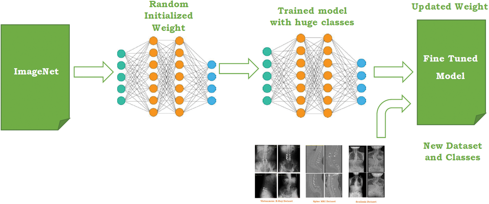
Figure 5: Transfer learning for the proposed work
To test the proposed approach, we collected the data from 3 different sources which include one local Vietnamese hospital and two public repositories (see Fig. 6). Vietnamese hospital dataset only includes 200 DICOM images that are not enough for the proposed approach. To overcome this issue, two different ways are being deployed.
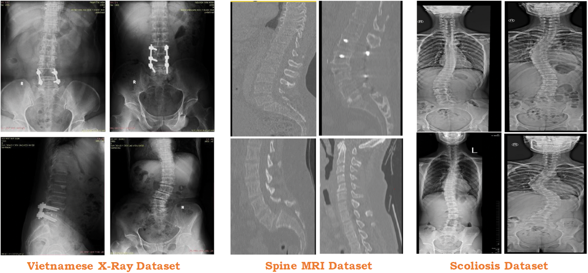
Figure 6: Usage of different dataset in the proposed study
4.1 Conversion of MRI Data Into 2D Imaging
MRI is an imaging technique to form a picture of human body parts and organs anatomy. MRI image covers 360-degree imaging of the human body organs which can store images in the form of several slices. These slices are 2D in nature but it can transform into 3D imaging with their combination. In the proposed approach (see Fig. 7), we convert the MRI file into the number of DICOM images or slices. However, one MRI imaging contains more than 200 slices but we consider only 2–3 imaging slices as per the need of the dataset.
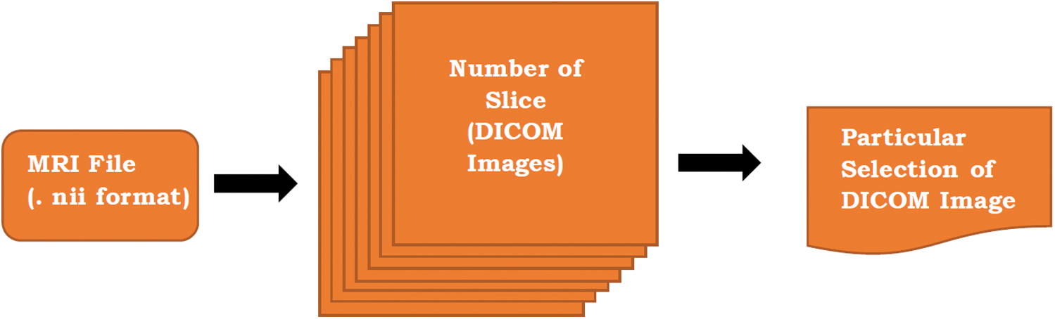
Figure 7: Conversion of MRI files into particular image
Similarly, in the case of Scoliosis detection, the Vietnamese Dataset and MRI Dataset [57] are also limited and not enough to predict scoliosis in the X-Ray imaging. To increase the number of scoliosis X-Ray imaging in the dataset, some images [58] are used. This dataset contains 98 scoliosis x-ray imaging which is suitable for our system.
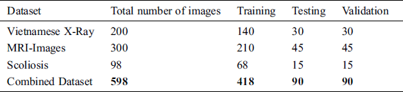
Tab. 4 represents the flow of dataset distribution in the proposed system. A total of 598 images have been used in the proposed system including 200 images, 300 images, and 98 images from the Vietnamese x-ray, MRI imaging, and scoliosis dataset respectively. 200 images in the Vietnamese x-ray are further divided into 140 images, 30 images, and 30 images for training, testing, and validation respectively. 300 images in the MRI-images are further divided into 210 images, 45 images, and 45 images for training, testing, and validation respectively. 98 images in the scoliosis are further divided into 68 images, 15 images, and 15 images for training, testing and, validation respectively.
Table 4: Flow of dataset distribution in the proposed system
The performance measures in the proposed study are accuracy, losses, sensitivity, and specificity which are explained in the following Section (Eqs. (2)–(4)). Accuracy is the percentage of prediction correct images over the test dataset. Sensitivity is used to measure the number of actual positive cases in the dataset that got predicted as accurately positive results. Specificity is used to measure the number of true negative cases in the dataset that got predicted as negative results.


where TP, TN, and FP stand for the True Positive. True Negative and False Positive. TP is the number of images that correctly identified the problems. TN is the number of images that are correctly identified as normal. FP is the number where X-Ray imaging incorrectly identified the wrong problem.
This section discusses the results obtained from our experimental setup. This experiment is done for two different approaches which are used in the proposed system as follows:
Our proposed system approach 1 performance is summarized in Tab. 5. In this approach, two pre-trained models are used and modified as per our dataset requirement.
Table 5: System performance with pre-trained models
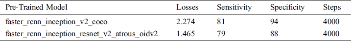
In the API models, sensitivity for the persons who have scoliosis and lumbar implant is 81% and 79% for the pertained models faster_rcnn_inception_v2_coco and faster_rcnn_inception_resnet_v2_atrous_oidv2 respectively. People who do not have these spinal problems, sensitivity for the faster_rcnn_inception_v2_coco and faster_rcnn_inception_resnet_v2_atrous_oidv2 models are 94% and 88 % respectively (see Fig. 8).
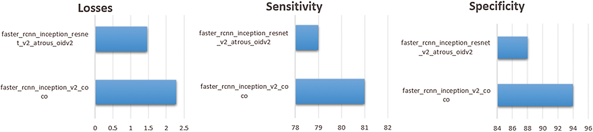
Figure 8: Comparison of pre-trained APIs models on the dataset
The number of steps used to train both models are 4000. One of the important parameters to measure the performance of the trained model is losses. Fewer losses in the models mean the system works more accurately but if there is very little loss, it signifies the system will face the overfitting problem. In our system, losses for the faster_rcnn_inception_v2_coco and faster_rcnn_inception_resnet_v2_atrous_oidv2 models are 2.274 and 1.465 respectively. If these values are less, maybe the system will perform better.
The proposed system performance measure for the second approach is discussed in Tab. 6. In this approach four different models are applied to find the suitable model for the system.
Table 6: System performance with transfer learning
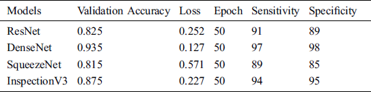
The validation accuracy of the ResNet, DenseNet, SqueezeNet and Inspection V3 are 0.825, 0.935, 0.815 and 0.875 respectively. The overall loss at the time of model training for the ResNet, DenseNet, SqueezeNet and Inspection V3 are 0.252, 0.127, 0.571 and 0.227 respectively (see Fig. 9). In every experiment, epoch values are fixed to 50 to achieve higher scores in the validation accuracy and loss. At the time of training the model, DenseNet achieved the highest score in validating accuracy as compared to other models. Similarly, in the case of losses, DenseNet achieved the lowest score as compared to other models. The sensitivity and specificity are important parameters that help to measure how the model behaves. The sensitivity of the combined dataset for the ResNet, DenseNet, SqueezeNet, and Inspection V3 are 91, 97, 89, and 94 respectively. The specificity of the combined dataset for the ResNet, DenseNet, SqueezeNet, and Inspection V3 are 89, 98, 85, and 95 respectively. DenseNet is the most suitable solution for the proposed solution.
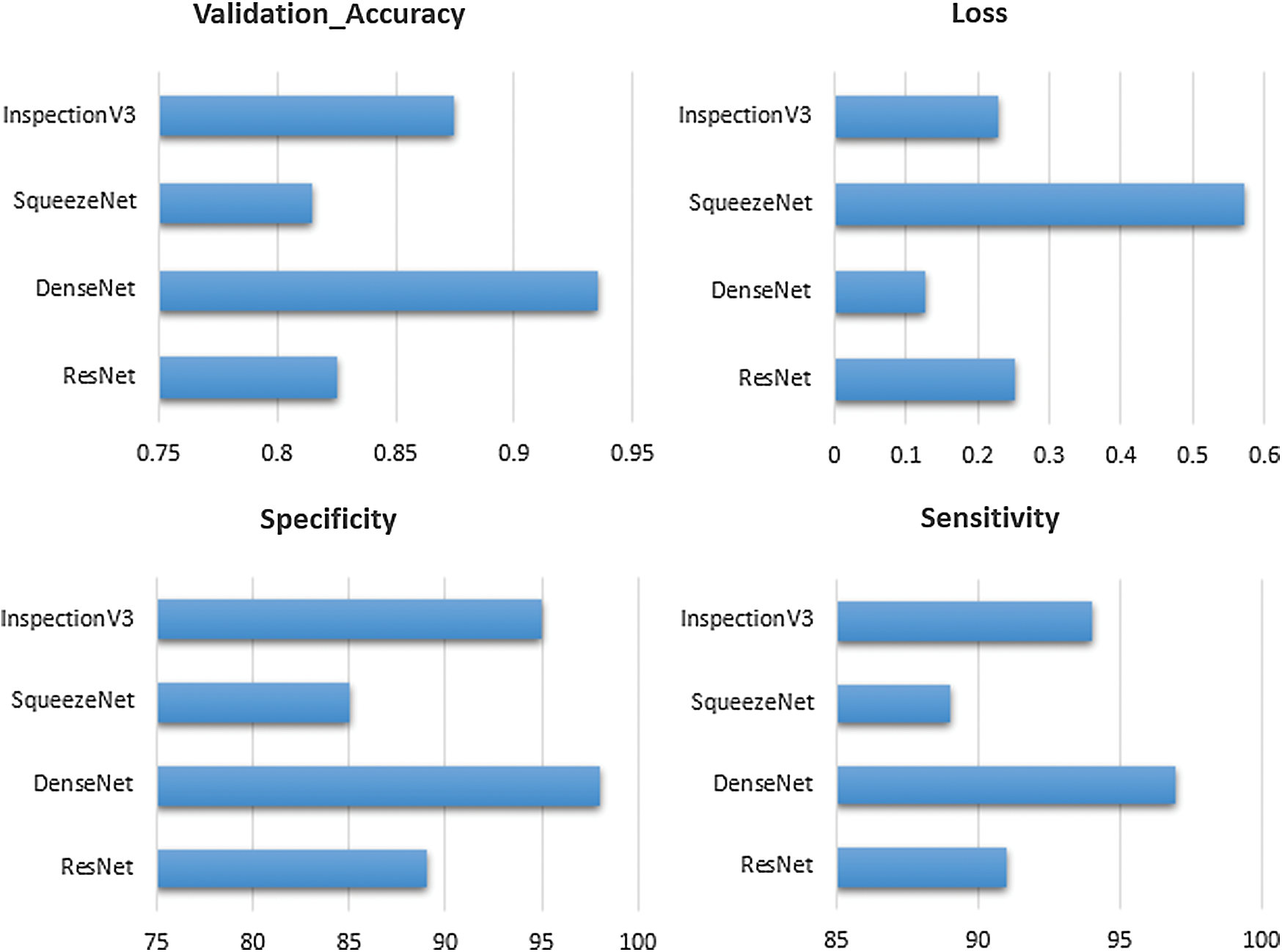
Figure 9: Comparison of transfer learning on the dataset
As per the results, the Transfer learning approach is a perfectly suitable solution for the proposed system as compared to the Pre-Trained API method. The training time in the transfer is much less as compared to the API method.
In this paper, we detected the lumbar implant and diagnosed scoliosis in the modified Vietnamese X-Ray imaging through the use of pre-trained model API and transfer learning. The collected dataset used in the study is the combination of Vietnamese X-ray imaging from the local hospital, conversion of MRI imaging to DICOM images, and public scoliosis dataset. Although, we achieved good validation accuracy, sensitivity, and specificity but it does not mean an out-of-box product for the healthcare industry. The main purpose of this study is to create autonomous objects detection and diagnosis systems for the radiologist, data scientist, and healthcare staff. In this proposed system, two different approaches are applied to check which approach is suitable for our proposed dataset. Transfer learning approaches are more suitable as compared to the pre-trained model API. Four models used in the transfer learning provide satisfied result outcomes as compared to the API models. In addition, transfer learning requires less time for model training and provides highly accurate results in small medical imaging dataset. DenseNet provides high validation accuracy 0.935 as compared to the ResNet with 0.825, SqueezeNet with 0.815, and InspectionV3 with 0.875 and selected for the proposed system.
Funding Statement: The authors received no specific funding for this study.
Conflicts of Interest: The authors declare that they have no conflicts of interest to report regarding the present study.
References
1. R. Buchbinder, M. V. Tulder, B. Öberg, L. M. Costa, A. Woolf et al. (2018). , “Low back pain: A call for action,” Lancet, vol. 391, no. 10137, pp. 2384–2388.
2. G. Fan, H. Liu, Z. Wu, Y. Li, C. Feng et al. (2019). , “Deep learning-based automatic segmentation of lumbosacral nerves on CT for spinal intervention: A translational study,” American Journal of Neuroradiology, vol. 40, no. 6, pp. 1074–1081.
3. J. D. Iannuccilli, E. A. Prince and G. M. Soares. (2013). “Interventional spine procedures for management of chronic low back pain-a primer,” “Seminars in Interventional Radiology, vol. 30, no. 3, pp. 307–317.
4. S. P. Cohen, S. Hanling, M. C. Bicket, R. L. White, E. Veizi et al. (2015). , “Epidural steroid injections compared with gabapentin for lumbosacral radicular pain: Multicenter randomized double-blind comparative efficacy study,” BMJ (Clinical Research ed.), vol. 350, pp. 1748.
5. F. Alonso and D. J. Hart. (2014). Intervertebral Disk. 2nd ed., Elsevier, pp. 724–729.
6. J. Krämer. (1990). Intervertebral disk diseases. Stuttgart: Thieme.
7. J. R. Coates. (2000). “Intervertebral disk disease,” Veterinary Clinics of North America: Small Animal Practice, vol. 30, no. 1, pp. 77–110.
8. I. Nozomu and A. A. E. Orías. (2011). “Biomechanics of intervertebral disk degeneration,” Orthopedic Clinics, vol. 42, no. 4, pp. 487–499.
9. Intervertebral Disk Diseases Details, U.S. National Library of Medicine. [Online]. Available: https://medlineplus.gov/genetics/condition/intervertebral-disc-disease/.
10. R. Fayssoux, N. I. Goldfarb, A. R. Vaccaro and J. Harrop. (2010). “Indirect costs associated with surgery for low back pain-A secondary analysis of clinical trial data,” Population Health Management, vol. 13, no. 1, pp. 9–13.
11. A. N. A. Tosteson, J. S. Skinner, T. D. Tosteson, J. D. Lurie, G. Anderson et al. (2008). , “The cost effectiveness of surgical versus non-operative treatment for lumbar disc herniation over two years: Evidence from the Spine Patient Outcomes Research Trial (SPORT),” Spine, vol. 33, no. 19, pp. 2108–2115.
12. D. Wildenschild, J. W. Hopmans, C. M. P. Vaz, M. L. Rivers, D. Rikard et al. (2002). , “Using x-ray computed tomography in hydrology: Systems, resolutions, and limitations,” Journal of Hydrology, vol. 267, no. 3–4, pp. 285–297.
13. M. C. Fu, R. A. Buerba, W. D. Long, D. J. Blizzard, A. W. Lischuk et al. (2014). , “Interrater and intrarater agreements of magnetic resonance imaging findings in the lumbar spine: Significant variability across degenerative conditions,” Spine Journal, vol. 14, no. 10, pp. 2442–2448.
14. S. Ghosh, M. R. Malgireddy, V. Chaudhary and G. Dhillon. (2012). “A new approach to automatic disc localization in clinical lumbar MRI: Combining machine learning with heuristics,” in 2012 9th IEEE Int. Sym. on Biomedical Imaging (ISBIBarcelona, pp. 114–117.
15. M. A. Larhmam, M. Benjelloun and S. Mahmoudi. (2014). “Vertebra identification using template matching modelmp and K-means clustering,” International Journal of Computer Assisted Radiology and Surgery, vol. 9, no. 2, pp. 177–187.
16. M. U. Ghani, F. Mesadi, S. D. Kanık, A. Argunşah, A. F. Hobbiss et al. (2017). , “Dendritic spine classification using shape and appearance features based on two-photon microscopy,” Journal of Neuroscience Methods, vol. 279, pp. 13–21.
17. M. U. Ghani, E. Erdil, S. U. Kanık, A. Ö. Argunşah, A. F. Hobbiss et al. (2016). , “Dendritic spine shape analysis: A clustering perspective,” in European Conf. on Computer Vision, Cham: Springer, pp. 256–273.
18. C. L. Hoad and A. L. Martel. (2002). “Segmentation of MR images for computer-assisted surgery of the lumbar spine,” Physics in Medicine & Biology, vol. 47, no. 19, pp. 3503.
19. J. Egger, C. Nimsky and X. Chen. (2017). “Vertebral body segmentation with GrowCut: Initial experience, workflow and practical application,” SAGE Open Medicine, vol. 5, no. 1, pp. 205031211774098.
20. A. Neubert, J. Fripp, C. Engstrom, R. Schwarz, L. Lauer et al. (2012). , “Automated detection, 3D segmentation and analysis of high-resolution spine MR images using statistical shape models,” Physics in Medicine & Biology, vol. 57, no. 24, pp. 8357.
21. Z. Peng, J. Zhong, W. Wee and J. Lee. (2005). “Automated vertebra detection and segmentation from the whole spine MR images,” in 2005 IEEE Engineering in Medicine and Biology 27th Annual Conf., Shanghai, China, pp. 2527–2530.
22. J. Yao, H. Munoz, J. E. Burns, L. Lu and R. M. Summer. (2014). “Computer aided detection of spinal degenerative osteophytes on sodium fluoride PET/CT,” in Computational Methods and Clinical Applications for Spine Imaging, Lecture Notes in Computational Vision and Biomechanics Book Series, J. Yao, T. Klinder, S. Li (eds.vol. 17, Cham: Springer, pp. 51–60.
23. M. Lootus, T. Kadir and A. Zisserman. (2014). “Radiological grading of spinal MRI,” in Recent Advances in Computational Methods and Clinical Applications for Spine Imaging, Springer, Cham, pp. 119–130.
24. Z. Liang, G. Zhang, J. X. Huang and Q. V. Hu. (2014). “Deep learning for healthcare decision making with EMRs,” in 2014 IEEE Int. Conf. on Bioinformatics and Biomedicine, Belfast, pp. 556–559.
25. P. Lakhani and B. Sundaram. (2017). “Deep learning at chest radiography: Automated classification of pulmonary tuberculosis by using convolutional neural networks,” Radiology, vol. 284, no. 2, pp. 574–582.
26. X. Wang, Y. Peng, L. Lu, Z. Lu, M. Bagheri et al. (2017). , “Automatic classification and reporting of multiple common thorax diseases using chest radiographs,” in Deep Learning and Convolutional Neural Networks for Medical Imaging and Clinical Informatics. Cham: Springer, pp. 393–412.
27. A. Esteva, B. Kuprel and R. Novoa. (2017). “Dermatologist-level classification of skin cancer with deep neural networks,” Nature, vol. 542, no. 7639, pp. 115–118.
28. L. Faes, S. K. Wagner, D. J. Fu, X. Liu, E. Korot et al. (2019). , “Automated deep learning design for medical image classification by health-care professionals with no coding experience: A feasibility study,” Lancet Digital Health, vol. 1, no. 5, pp. e232–e242.
29. O. Stephen, M. Sain, U. J. Maduh and D.U. Jeong. (2019). “An efficient deep learning approach to pneumonia classification in healthcare,” Journal of Healthcare Engineering, vol. 2019, no. 1, pp. 7.
30. A. Suzani, A. Seitel, Y. Liu, S. Fels, R. N. Rohling et al. (2015). , “Fast automatic vertebrae detection and localization in pathological ct scans-a deep learning approach,” in Int. Conf. on Medical Image Computing and Computer-Assisted Intervention, Cham: Springer, pp. 678–686.
31. W. Whitehead, S. Moran, B. Gaonkar, L. Macyszyn and S. Iyer. (2018). “A deep learning approach to spine segmentation using a feed-forward chain of pixel-wise convolutional networks,” in IEEE 15th Int. Sym. on Biomedical Imaging, Washington, DC, pp. 868–871.
32. F. Galbusera, F. Niemeyer, H. J. Wilke, T. Bassani, G. Casarol et al. (2019). , “Fully automated radiological analysis of spinal disorders and deformities: A deep learning approach,” European Spine Journal, vol. 28, no. 5, pp. 951–960.
33. R. Sa, W. Owens, R. Wiegand, M. Studin, D. Capoferri et al. (2017). , “Intervertebral disc detection in X-ray images using faster R-CNN,” in 2017 39th Annual Int. Conf. of the IEEE Engineering in Medicine and Biology Society, Seogwipo, pp. 564–567.
34. C. Kuok, M. Fu, C. Lin, M. Horng, Y. Sun et al. (2018). , “Vertebrae segmentation from x-ray images using convolutional neural network,” in Proc. the 2018 Int. Conf. on Information Hiding and Image Processing, Manchester United Kingdom, pp. 57–61.
35. K. C. Kim, H. C. Cho, T. J. Jang, J. M. Choi, J. K. Seo et al. (2019). , “Automatic detection and segmentation of lumbar vertebra from X-ray images for compression fracture evaluation. arXiv preprint arXiv:1904.07624.
36. D. Forsberg, E. Sjöblom and J. L. Sunshine. (2017). “Detection and labeling of vertebrae in MR images using deep learning with clinical annotations as training data,” Journal of Digital Imaging, vol. 30, no. 4, pp. 406–412.
37. V. Bhateja, A. Moin, A. Srivastava, L. N. Bao, A. Lay-Ekuakille et al. (2016). , “Multispectral medical image fusion in Contourlet domain for computer based diagnosis of Alzheimer’s disease,” Review of Scientific Instruments, vol. 87, no. 7, 074303.
38. C. Le Van, G. N. Nguyen, T. H. Nguyen, T. S. Nguyen and D. N. Le. (2020). “An effective RGB color selection for complex 3D object structure in scene graph systems,” International Journal of Electrical and Computer Engineering (IJECE), vol. 10, no. 6, pp. 5951–5964.
39. S. F. Qadri, A. Danni, H. Guoyu, M. Ahmad, Y. Huang et al. (2019). , “Automatic deep feature learning via patch-based deep belief network for vertebrae segmentation in CT images,” Applied Science, vol. 9, no. 1, pp. 2076–3417.
40. G. Fan, H. Liu, Z. Wu, Y. Li, C. Feng et al. (2019). , “Deep learning-based automatic segmentation of lumbosacral nerves on CT for spinal intervention: A translational study,” American Journal of Neuroradiology, vol. 40, no. 6, pp. 1074–1081.
41. C. Buerger, J. V. Berg, A. Franz, T. Klinder, C. Lorenz et al. (2020). , “Combining deep learning and model-based segmentation for labeled spine CT segmentation,” Medical Imaging 2020: Image Processing, vol. 11313, 113131C.
42. J. Zhao, Z. Jiang, K. Mori, L. Zhang, W. He et al. (2019). , “Spinal vertebrae segmentation and localization by transfer learning,” Medical Imaging 2019: Computer-Aided Diagnosis, vol. 10950, pp. 1095023.
43. M. Raghu, C. Zhang, J. Kleinberg and S. Bengio. (2019). “Transfusion: Understanding transfer learning for medical imaging,” Advances in Neural Information Processing Systems, vol. 32, pp. 3347–3357.
44. J. Huang, V. Rathod, C. Sun, M. Zhu, A. Korattikara et al. (2017). , “Speed/Accuracy trade-offs for modern convolutional object detectors,” in Proc. the IEEE Conf. on Computer Vision and Pattern Recognition, Honolulu, HI, USA, vol. 32, pp. 7310–7731, July.
45. A. M. Taqi, F. A. Azzo, A. Awad and M. Milanova. (2019). “Skin lesion detection by android camera based on ssd-mo-bilenet and tensorflow object detection API,” American Journal of Advanced Research, vol. 3, no. 1, pp. 5–11.
46. S. Ren, K. He, R. Girshick and J. Sun. (2015). “R-CNN Faster: Towards real-time object detection with region proposal networks,” IEEE Transactions on Pattern Analysis & Machine Intelligence, vol. 6, pp. 1137–1149.
47. K. He, X. Zhang, S. Ren and J. Sun. (2016). “Deep residual learning for image recognition,” in Proc. the IEEE Conf. on Computer Vision and Pattern Recognition, Las Vegas, NV, USA, pp. 770–778, June.
48. G. Huang, Z. Liu, L. Maaten and K. Q. Weinberger. (2017). “Densely connected convolutional networks,” in Proc. IEEE Conf. on Computer Vision and Pattern Recognition, Honolulu, HI, USA, pp. 4700–4708, July.
49. C. Szegedy, W. Liu, Y. Jia, P. Sermanet, S. Reed et al. (2015). , “Going deeper with convolutions,” in Proc. the IEEE Conf. on Computer Vision and Pattern Recognition, pp. 1–9.
50. G. Kobayashi and H. Shouno. (2020). “Interpretation of ResNet by visualization of preferred stimulus in receptive fields. arXiv preprint arXiv:2006.01645.
51. C. Szegedy, V. Vanhoucke, S. Ioffe, J. Shlens and Z. Wojna. (2016). “Rethinking the inception architecture for computer vision,” in Proc. the IEEE Conf. on Computer Vision and Pattern Recognition (CVPRLas Vegas, NV, USA, pp. 2818–2826.
52. F. N. Iandola, S. Han, M. W. Moskewicz, K. Ashraf, W. J. Dally et al. (2016). , “Squeeze Net: AlexNet-level accuracy with 50x fewer parameters and <0.5 MB model size. arXiv preprint arXiv: 1602.07360.
53. K. Simonyan and A. Zisserman. (2014). “Very deep convolutional networks for large-scale image recognition. arXiv preprint arXiv: 1409.1556.
54. Tensorflow Models Garden. [Online]. Available: https://github.com/tensorflow/models.
55. P. Singh and A. Manure. (2020). “Neural networks and deep learning with TensorFlow,” in Learn TensorFlow 2.0. Berkeley, CA: Apress, pp. 53–74.
56. ImageNet Database, Stanford Vision Lab, Stanford University, Princeton University. [Online]. Available: http://www.image-net.org/.
57. S. Sudirman, A. A. Kafri, F. Natalia, H. Meidia, N. Afriliana et al. (2019). , “Label image ground truth data for lumbar spine MRI dataset,” Mendeley Data, . [Online]. Available: https://data.mendeley.com/datasets/zbf6b4pttk/1.
58. Scoliosis Test Dataset, Accurate Automated Spinal Curvature Estimation 2019. [Online]. Available: https://aasce19.github.io/.
 | This work is licensed under a Creative Commons Attribution 4.0 International License, which permits unrestricted use, distribution, and reproduction in any medium, provided the original work is properly cited. |