Computers, Materials & Continua DOI:10.32604/cmc.2020.012328
Article

Straw Segmentation Algorithm Based on Modified UNet in Complex Farmland Environment

Yuanyuan Liu1,2, Shuo Zhang1, Haiye Yu3, Yueyong Wang4,*, Yuehan Feng1, Jiahui Sun1 and Xiaokang Zhou1

1College of Information Technology, Jilin Agriculture University, Changchun, 130118, China
2Department of Biosystems and Agricultural Engineering, Oklahoma State University, Stillwater, 74078, USA
3Key Laboratory of Bionic Engineering, Ministry of Education, Jilin University, Changchun, 130025, China
4College of Engineering and Technology, Jilin Agricultural University, Changchun, 130118, China
*Corresponding Author: Yueyong Wang. Email: yueyongw@jlau.edu.cn
Received: 25 June 2020; Accepted: 22 July 2020

Abstract: Intelligent straw coverage detection plays an important role in agricultural production and the ecological environment. Traditional pattern recognition has some problems, such as low precision and a long processing time, when segmenting complex farmland, which cannot meet the conditions of embedded equipment deployment. Based on these problems, we proposed a novel deep learning model with high accuracy, small model size and fast running speed named Residual Unet with Attention mechanism using depthwise convolution (RADw–UNet). This algorithm is based on the UNet symmetric codec model. All the feature extraction modules of the network adopt the residual structure, and the whole network only adopts 8 times the downsampling rate to reduce the redundant parameters. To better extract the semantic information of the spatial and channel dimensions, the depthwise convolutional residual block is designed to be used in feature maps with larger depths to reduce the number of parameters while improving the model accuracy. Meanwhile, the multi–level attention mechanism is introduced in the skip connection to effectively integrate the information of the low–level and high–level feature maps. The experimental results showed that the segmentation performance of RADw–UNet outperformed traditional methods and the UNet algorithm. The algorithm achieved an mIoU of 94.9%, the number of trainable parameters was only approximately 0.26 M, and the running time for a single picture was less than 0.03 s.

Keywords: Straw segmentation; convolutional neural network; residual structure; depthwise convolution; attention mechanism

1  Introduction

Returning straw to a field is a conservation tillage measure that is widely valued around the world today. Straw return can not only eliminate the air pollution caused by straw burning but also increase fertilizer and crop yields and reduce greenhouse gas emissions [1–3]. Therefore, straw mulching has a positive impact on agricultural production and the ecological environment. To better limit straw burning and guide farmers to reasonably return straw to fields, it is necessary to quantitatively evaluate the straw returning rate. Therefore, the detection of the straw coverage rate in fields is particularly important.

To accurately and quickly calculate the straw coverage rate, it is highly valuable to solve this problem using computer vision technology that has rapidly developed in recent years. The technology has the characteristics of low cost, high efficiency and large economic benefits. However, this method is usually carried out by unmanned aerial vehicles (UAVs) with cameras, which brings many problems. For example, because the field environment is generally complicated, there are usually disturbances such as vegetation, roads, agricultural machinery, and houses around fields. Especially, the surrounding trees cast long shadows over fields under the hot sun. These interference factors may appear in the pictures taken by a UAV, resulting in increased processing difficulty and decreased accuracy. To solve the problem of difficult straw detection in complex scenes, the most important thing is to separate these objects, which can strongly reduce the interference.

The most common traditional segmentation method is threshold segmentation. For example, Wang et al. [4] proposed a method combining the Sauvola and Otsu algorithms to detect the straw area in a detailed image. Li et al. [5] proposed a method combining texture features with a BP neural network to identify straw and soil, but the detection time was up to 10 s. Therefore, Liu et al. [6] proposed straw coverage detection based on a multi–threshold image segmentation algorithm and used the DE–GWO algorithm to conduct multi–threshold image segmentation. The detection accuracy reached more than 95%, and the test time for a single picture was shortened to less than 2 s; however, the stability of the algorithm was not good. The above segmentation algorithms based on a threshold value all have the same problem, that is, objects with similar colors may be classified into one class. However, the texture–based algorithm needs to manually design features, which greatly increases the difficulty of the algorithm’s development. In addition, the above algorithms are not effective for complex farmland, especially when the images are subject to interference caused by the tree shadows.

In recent years, due to the development of deep learning, Hinton et al. [7] significantly reduced the error rate of ImageNet image classification to 16% in the 2012 ILSVRC competition by using convolutional neural network. Then the convolutional neural network was widely used in the fields of image recognition [8–14], object detection [13–17], image segmentation [18–22] and so on. Among them, the use of fully convolutional network to solve the semantic segmentation problem was proposed by Jonathan Long et al. [23], which was the first to use fully convolutional network to solve the semantic segmentation problem. As the convolutional neural network can automatically extract the features of each class through learning a large amount of data, it has a significant classification effect on images, and the segmentation effect for complex scenes is obviously better than the traditional segmentation based on texture or threshold. For example, Liu et al. [24] designed DSRA–UNet deep convolutional neural network, which can accurately segment up to 6 classes of farmland scene, and the segmentation effect of straw was not disturbed by other classes, so the segmentation result was better, and the shadow problem can be solved to some extent. However, there are still many training parameters in this algorithm, and the effect of shadow segmentation on straw still needs to be improved. Based on this, a new segmentation network was designed to solve the problem of straw coverage detection in complex scenes. Overall architecture adopted the design idea of UNet [25] symmetry—decoding. It was a whole residual network [26] architecture, and use the Depthwise Convolution [27] to reduce the number of parameters. At the same time, attention mechanism [28–32] was designed to focus on integral pixel hard. Through the above operation, the network in a very low number of parameters and shallow depth, and only 8 times down sampling cases still can achieve higher precision. The proposed algorithm was tested on the straw data set, and it can achieve better segmentation effect under different lighting environment, camera shooting height and scene complexity. At the same time, the network is end–to–end trainable and has a small number of parameters, which makes its model small in size and fast in operation, and greatly reduces the difficulty of deploying to embedded devices. Therefore, the algorithm is very conducive to on–site real–time detection in an environment with few electronic devices such as farmland.

2  Proposed Method

2.1 Model Analysis and Overview

Straw coverage detection is based on computer vision technology. In this technology, the image is acquired by aerial photography using a UAV, and then the image is preprocessed and input into the convolutional neural network to obtain the prediction map. As shown in Fig. 1, the complex field scene includes straw, soil, road, the surrounding vegetation, agricultural machinery, tree shadows and other interfering factors. If there is no disturbance in the field, the field only contains straw, grass and soil. Since the amount of grass is relatively little and most of it is covered by straw, the grass and soil are classified into one class. Regarding the interference of farm machinery and tree shadows in the field (it can be seen from the figure that the influence range of tree shadows is larger than any other), it is difficult to divide the area because of the shadows of the trees on the straw; therefore, it is easy to identify the straw covered with tree shadows as soil.

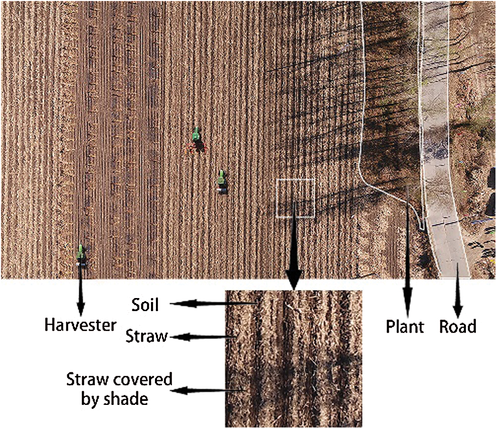
Figure 1: Schematic diagram of complex field scene

To accurately segment straw, this paper used a convolutional neural network to extract the straw characteristics and proposed a new segmentation network called RADw–UNet. The network is based on UNet’s symmetric codec semantic segmentation model, in which the low–level feature layer uses the standard convolution and the high–level feature layer uses the depthwise convolution to construct the entire network architecture. Meanwhile, a large number of 1 × 1 convolutions are used to increase the dimension to reduce the number of training parameters. In addition, the residual structure is added in the two convolution processes of each layer to increase the depth and feature expression ability of the network. Finally, the attention mechanism is added to obtain more accurate information before the skip connection. Through the above operation, the straw segmentation ability can be improved by reducing the network parameters and depth to adapt to the complex farmland scene.

2.2 RADw–UNet Algorithm

The network architecture proposed in this paper is shown in Fig. 2, where the depth of the feature map is marked above the feature map. The number in the circle is the number of feature extraction modules in each layer, and the meaning of each symbol is marked in the dotted box. This architecture uses only three downsampling layers instead of the four in the original UNet. The purpose is to reduce the number of parameters in the network and to increase the ability of the network to obtain global information. Again, it is going to be upsampled after three deconvolutions. Layers 1–3 in the lower sampling process are connected with layers 6–8 in the upper sampling by a skip connection. In the coding stage, the first layer uses the residual blocks of the standard convolution for feature extraction. The second to fourth layers use the max pooling to reduce the dimensionality, and then use the depthwise convolutional residual blocks to perform downsampling feature extraction. Finally, a feature map with the horizontal size decreased eightfold and the depth expanded to 128 will be obtained. In the decoding stage, a multi–level attention mechanism is added to increase the semantic information in the low–level feature map before the skip connection, and then a 1 × 1 convolution is carried out, which is spliced with the deconvolved feature map of the upper layer to combine the downsampling and upsampling information with the same scale. After the splicing is completed, feature fusion is carried out through the depthwise convolutional residual block. After the third upsampling, the spliced feature map is passed through the standard convolutional residual block, and then the prediction map that is the same size as the input picture is obtained through the 1 × 1 convolution and softmax function.

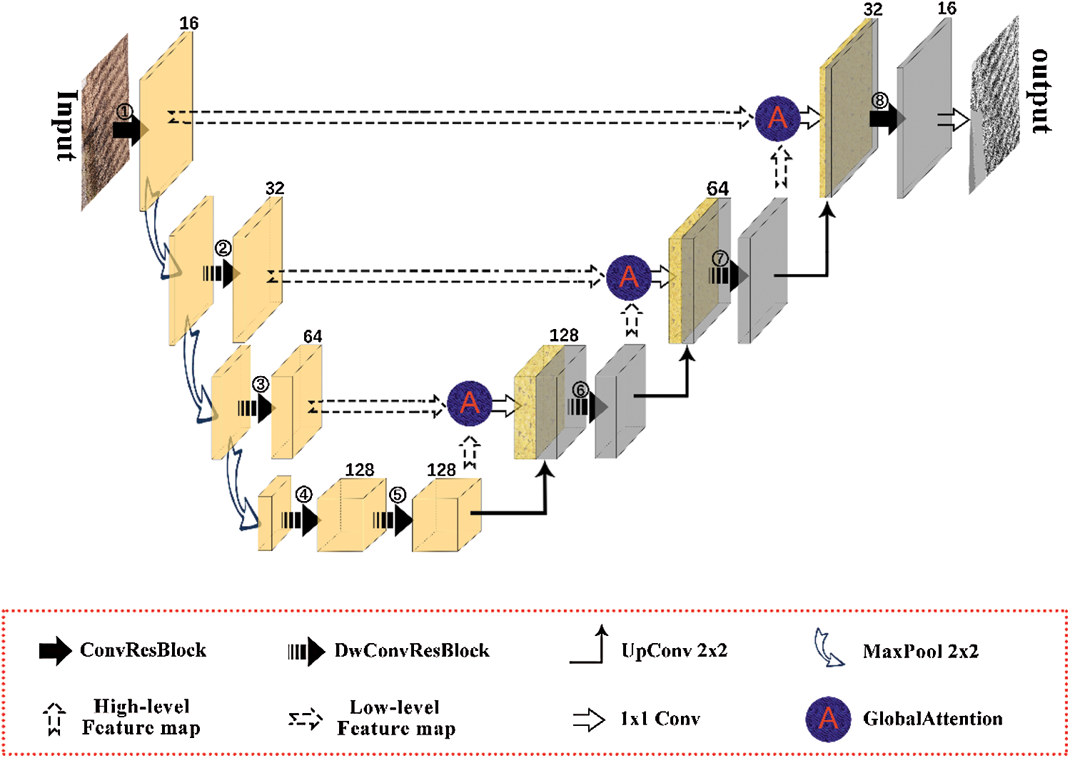
Figure 2: Network architecture of RADw–UNet algorithm

2.3 Standard Convolutional Residual Block

The residual network [26–33] can not only solve the disappearing gradient and exploding gradient problems caused by the deep network but can also fuse the input information into the network through a shortcut to make the network deeper. Thus, the network can be deepened when the network depth is shallow to enhance the feature expression capability. This module in Fig. 3 adds a residual structure on the basis of the standard convolution. Both convolution layers use a 3 × 3 convolution kernel and the ReLU activation function. The residual structure adds the input feature map after a 1 × 1 convolution kernel to the output of the two convolution layers to obtain the output result of this layer. This module is mainly used to extract the semantic information of high–resolution feature maps because high–resolution maps are generally shallow in depth and a large amount of information is stored in their spatial dimension; in addition, the standard convolution can better extract spatial dimension information than the depthwise convolution. Therefore, it is used in the feature extraction of the first layer and the last layer with a large size and shallow depth.

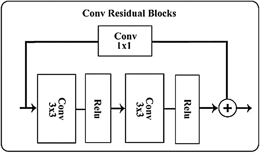
Figure 3: Standard convolution residual blocks

2.4 Depthwise Convolutional Residual Block

Different from the standard convolution operation, a depthwise convolution kernel [34] is only responsible for one channel, and the feature map with the same number of channels in the input layer is obtained without changing the depth of the feature map. This module is shown in Fig. 4. After the input feature maps are convoluted with two depthwise convolutions, their feature maps are concatenated and spliced such that the number of channels of the feature maps at this time will be doubled, and then feature fusion is carried out through a 1 × 1 convolution. In this process, two feature maps that have passed through the depthwise convolution are spliced to fuse semantic information with different complexity, which is more conducive to extracting features with different complexity from modules. Meanwhile, the depth of the feature map does not change during the depthwise convolution, but the network depth increases after splicing. This effect greatly reduces the network size, but it also decreases the precision due to the lack of training parameters. Therefore, this block uses a 5 × 5 convolution kernel to extract more information. Meanwhile, the residual structure is added to enhance the feature extraction capability. Since depthwise convolution extracts features from different depths separately, it has a better ability to obtain depth information. To use the depthwise convolution efficiently, it is used in the feature extraction stage of the high–level feature map from the second to the seventh layer in this paper.

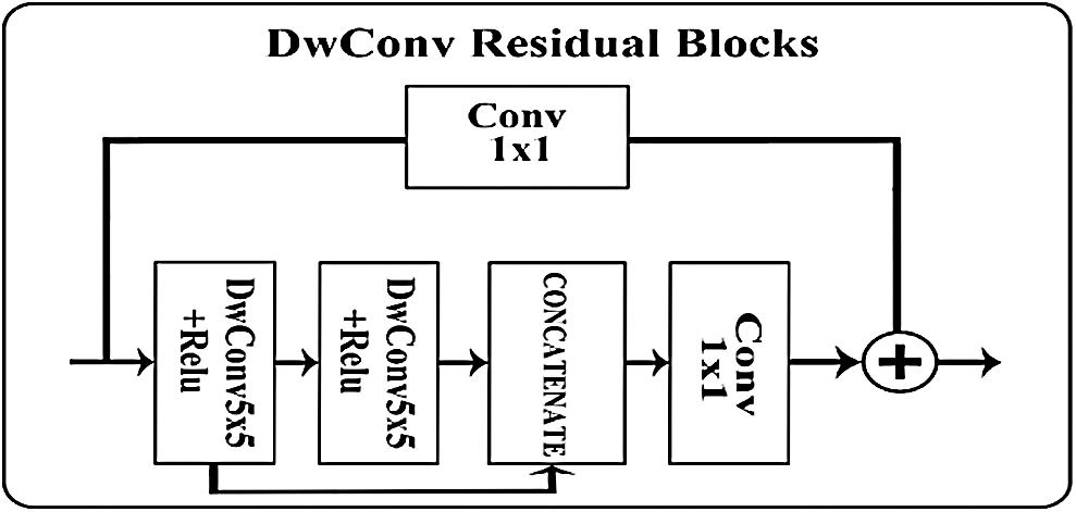
Figure 4: Depthwise convolution residual blocks

2.5 Multi–Level Attention Mechanism

Attention mechanisms have been widely used in natural language processing, image classification and other fields [28,29]. In recent years, they have also been applied to semantic segmentation and achieved good results [30,31]. Inspired by the attention upsample module in literature [32] and the Squeeze–and–Excitation module in the literature [35], we form the attention mechanism proposed in this paper, and it is shown in Fig. 5. Since the low–level feature map contains more location information while the high–level feature map contains rich class information, a more accurate feature map can be obtained by weighting the low–level features with more abundant class information. Therefore, this paper uses the rich semantic information in the high–level feature map to select the features for the low–level feature map to add more details to the low–level feature map. This approach enables more useful contextual information to be extracted at different levels.

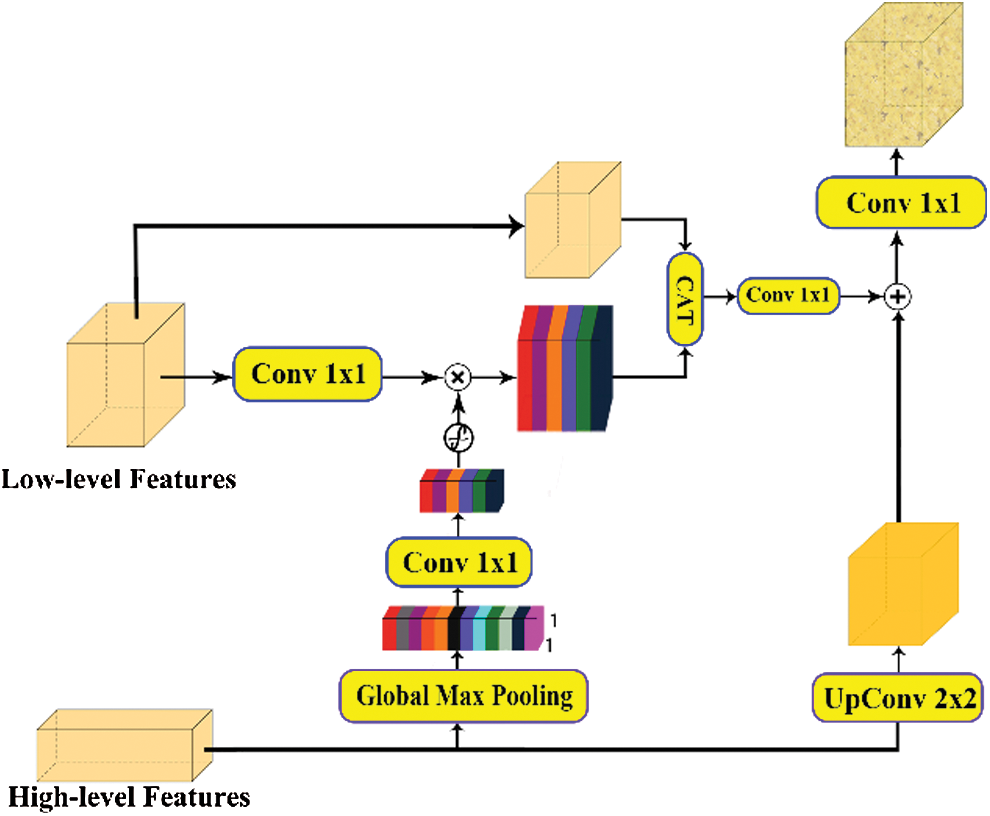
Figure 5: Multi–level Attention Mechanism

Due to the features of the figure, after the max pooling, we can obtain more important information under the current receptive field. The high–level feature map after the global max pooling obtains 1 × 1 × N feature vectors that provide the global context information. Again, after a 1 × 1 convolution, the ReLU reduces the dimension of the low level features. Finally, through a sigmoid activation function, the feature vector is mapped to the range of 0–1 to obtain the weight coefficient of each channel. Then, the weighted feature map is obtained by multiplying the weights by the low–level features that have passed the 1 × 1 convolution operation to obtain the importance of different channels and improve the feature expression ability of useful channels through learning. In addition, the weighted feature map is spliced with the low–level feature map, and the number of channels is reduced by half using a 1 × 1 convolution operation in order to fuse the input information with the weighted information. Finally, the high–level feature map is deconvolved to obtain the same shape as the low–level feature map, and the final filtered feature map is obtained by adding the weighted feature map.

3  Network Training and Optimization

3.1 Data Pre–Processing

This dataset was taken by a DJI wu2 generation UAV in Daigang township, Yushu city, Jilin Province in October 2018. Since straw is produced only after the autumn harvest, the number of samples is notably small. There are only 120 valid data samples, of which 100 are captured via a 2–minute video every 1.2 s. However, these 100 pictures are only single straw field images, lacking interfering factors, such as agricultural machinery, road, plants and tree shadows. Only the remaining 20 pictures contain these complex interferences, as shown in Fig. 6.

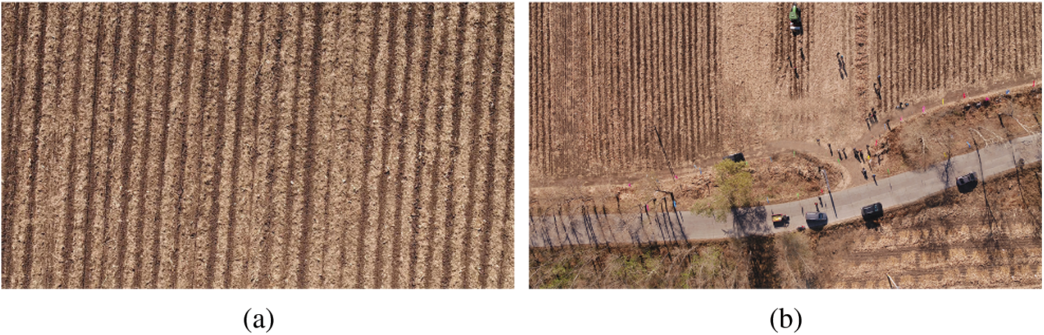
Figure 6: (a) Image of only straw; (b) Image of complex scene

Therefore, it is necessary to augment the data, improve the robustness of the network, and enhance the network segmentation of complex scenes. Since most of the images do not contain interference, new images need to be synthesized by adding interference to the 100 images containing only soil and straw. First, the pictures containing road, plants, houses and other interferences are synthesized. The main method is to cut out the road, plant, farm machinery and house in 20 pictures with interference and then add them to the pictures without interference and perform some operations, such as rotation and scaling, to produce pictures containing multiple categories of interference. Regarding tree shadows, it is difficult to cut tree shadows from the original images for image synthesis because the data set is small and the tree shadows are transparent. Therefore, this paper uses Photoshop to generate a large number of tree shadows and then adds them to 200 basic images. Through the above methods, 600 composite maps were obtained, and the 600 composite maps and 100 original images containing only straw land were used as the data set.

3.2 Loss Function

The cross–entropy loss (CE loss) function is often used in multi–classification, since it has the characteristic of fast convergence. However, the loss function is easily affected by unbalanced categories. Therefore, an equilibrium factor is introduced to solve the unbalanced category problem and make the network more focused on straw segmentation. The formula is defined as follows:

In the above formula, is the value of the loss function, is the number of classes, is the true value of the –th pixel of the –th class, is the probability that the –th pixel is predicted to be the –th class, and is the weight of the –th class. Since the four interference categories of agricultural machinery, highways, houses and vegetation have similar proportions in the images and their occurrence frequencies are small, the weight of all of them is 0.1. Straw is the focal class of this algorithm. The coverage and colour of straw are close to those of soil. Therefore, the weight of soil is 0.3, and the weight of straw is 0.8. The combined effect of these weights is the best after the experimental test. Through this balance, the network can pay more attention to the straw pixel information and produce a better segmentation effect for the shaded straw.

3.3 Training Hyperparameters

1.Optimizer: Adam

2.Learning–rate: The initial learning rate was 0.001, the decay coefficient was 0.5, and the minimum was 1e–8.

3.Batch size:1

4.Training epochs:125

5.Steps per epoch:560

4  Results and Discussion

The above algorithm was qualitatively and quantitatively evaluated on the straw data. The algorithm was trained and tested in an environment with Ubuntu18+python3.6+tensorflow1.10+ Keras2.2.0, and the training time was approximately 3 hours with an Nvidia GTX 1080 graphics card.

4.1 Evaluation Index

To better evaluate the straw coverage accuracy, this paper uses the straw coverage , the straw coverage error and the straw Intersection–over–Union to measure the performance of the algorithm.

4.1.1 Straw Coverage Error

The predicted straw coverage is defined as:

The actual straw coverage is defined as:

The error of straw coverage was obtained from Eqs. (2) and (3):

In the above formula, is the actual straw coverage rate. H is the picture height. W is the width of the picture, is the predicted number of straw pixels, and is the true number of real straw pixels.

4.1.2 Straw Intersection–over–Union

The straw Intersection–over–Union can reflect the relationship between the predicted straw and the real straw, which is an important index to measure the straw segmentation accuracy. The formula is defined as follows:

In the formula, is the number of intersecting pixels, is the predicted number of straw pixels, and is the actual number of straw pixels.

4.2 Effect Comparison of Different Algorithms

To verify the effectiveness of the algorithm proposed in this paper, the algorithm was compared with other algorithms, and the results are shown in Tab. 1. It can be seen from the table that the performances of SegNet [36] and Deeplab [37] in these data set were not good. The number of parameters for both of them was high, and the FPS was low. The UNet algorithm used a 3 × 3 convolution kernel size for all convolutions, and its maximum depth was 512. The precision reached 87.47% and the number of parameters was 7.8 M after 4 times downsampling. However, due to its simple network structure, the FPS was relatively high. DE–GWO [6] is a traditional threshold segmentation algorithm, which had a poor detection effect on complex scenes with shadows and a lower mIoU. The DSRA–UNet [24] algorithm achieved an mIoU of 94.1%, the number of parameters was reduced to 0.76 M, and it had a high FPS. The proposed algorithm increased the mIoU up to 94.9%, the number of parameters was only 0.26 M, and the FPS reached 34, which were better than other methods mentioned above.

Table 1: Comparison of different algorithms

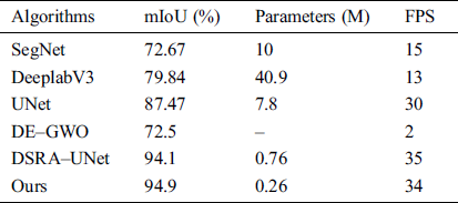
Fig. 8 shows the straw detection results of the proposed algorithm in different scenarios and its comparison with other algorithms. The grey level corresponding to the category is shown in Fig. 7.

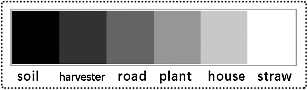
Figure 7: The grayscale color corresponding to each category

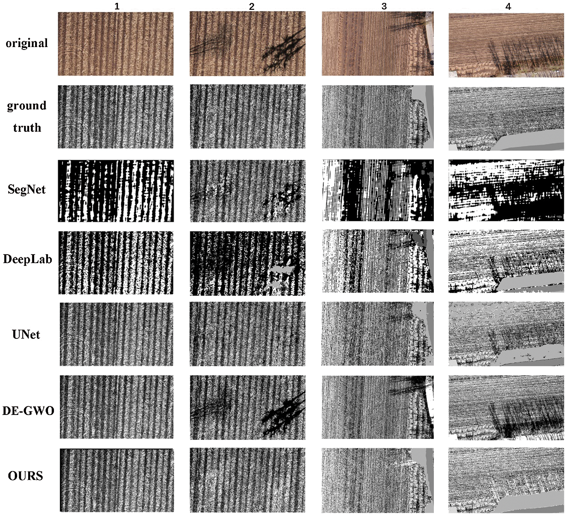
Figure 8: Experimental results of different algorithm

Fig. 8 shows the original figure, the ground truth and the prediction results of various algorithms from top to bottom, and it shows the straw coverage detection effect under different straw scenarios from left to right. For the first simplest scenario, the straw detection difficulty is relatively low, and most of the algorithms can detect the straw correctly; however, SegNet’s detection effect is not good. The second is a scene with tree shadows. It can be seen from the figure that the traditional algorithm has a weak detection effect for the tree shadows that covered straw. SegNet can detect part of the straw, while UNet and the algorithm proposed in this paper can segment most of the straw covered by shadows. Images three and four are complex farmland scenes. It can be seen from the figure that there are large areas with errors in the other methods, especially around roads, vegetation and tree shadows. The algorithm proposed in this paper can better segment the interferences and improve the straw coverage detection accuracy.

4.3 Basal Architecture Contrast

To verify the effectiveness of the proposed network architecture, two comparative experiments was designed. The first set of experiments was used to verify the effectiveness of using the standard convolutional residual block in the low–level feature map and the depthwise convolutional residual block in the high–level feature map. The second set was used to verify the effect of different decreasing sampling multiples on the model.

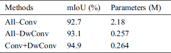
4.3.1 Convolution Type Contrast

For the high resolution feature map (such as the input three–channel picture and the feature map obtained after the last upsampling), the horizontal size is large, the depth is shallow, and most of its information is stored in the spatial dimension. Therefore, this paper used the standard convolution residual block in the high–resolution and low–depth feature map and used the depthwise convolutional residual block the low–resolution and high–depth feature map. The experimental results are shown in Tab. 2, where the other parameters remained unchanged and only the type of convolution was changed. All–Conv refers to the use of only the standard convolutional residual block. All–DwConv refers to the use of only the depthwise convolutional residual block. Conv+DwConv means that the standard convolutional residual block is used in the shallow layer and the depthwise convolutional residual block is used in the deep layer. It can be seen from the table that when only the standard convolution was used, the model resulted in an mIoU of 92.7% with high precision, but the number of parameters was approximately 8 times that of other methods. When only the depthwise convolution was used, the mIoU improved to 93.1%, and the number of parameters was only 0.257 M. When the structure proposed in this paper was adopted, the mIoU reached 94.9%, and the number of parameters increased by only approximately 0.007 M compared with the previous one, but the precision improved by 1.8%. Thus, the standard convolution can extract spatial information better and is suitable for use in high–resolution feature maps. The depthwise convolution can extract the high depth feature map better because the feature map of each channel can be extracted by the convolution, which has a high utilization rate for depth information. Therefore, the proposed structure can make full use of spatial information and depth information to achieve a balance between the number of parameters and the precision.

Table 2: Comparison of results from different convolution

4.3.2 Comparison of Different Downsampling Multiples

For a deep convolutional neural network, different downsampling multiples may determine the depth and horizontal dimension of the network. It is not necessarily true that the deeper the depth is, the higher the sampling ratio is, and the better the effect. In this experiment, in order to verify this, the results of different downsampling multiples are shown in Tab. 3. Pooling–4 represents 2 such downsamplings, that is, the maximum pooling layer with a step size of 2 is passed through twice. Although the number of parameters is small, the accuracy is not high due to the shallow network. Maximum pooling is carried out 4 times in Pooling–16. As the number of downsamplings is increased, the depth of the network is also increased, resulting in number of network parameters increasing to 0.99 M and an obvious accuracy improvement. Pooling–8 is the downsampling multiple adopted in this paper. The horizontal size is reduced to 8 times the original size, the number of parameters is reduced to 0.26 relative to Pooling–16, and the mIoU is also improved to some extent. This shows that, for different tasks, a deeper network does not necessarily result in better performance. In contrast, choosing an appropriate downsampling ratio can make the accuracy and model size both optimal.

Table 3: Comparison of results from different convolution

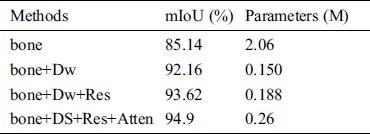
4.4 Comparison of Different Modules

To study the role of each module in the algorithm proposed in this paper, four different networks were designed, and their effects were compared. The experimental results are shown in Tab. 4. The first one is the backbone network. Since the middle layer (i.e., the second and seventh layers) used a 5 × 5 standard convolution, this part had a high number of parameters. However, due to the simplistic model, the mIoU was only 85.14%. The second part changed the middle layer to a depth convolution, thus greatly reducing the number of model parameters. However, the feature extraction ability of the network was greatly increased due to the addition of a depthwise convolution block, and it achieved an mIoU of 92.16%. The third part added a residual structure in both the upper and lower sampling, and the mIoU was increased to 93.62%. The fourth part introduced a multi–level attention mechanism. It can be seen from the table that the precision had been further improved after the introduction of this mechanism, and the number and precision of the parameters can be well balanced. The mIoU reached a maximum of 94.9%, and the number of parameters was only 0.26 M.

Table 4: Comparison of results from different modules

4.5 Field Test Sesults

This algorithm was applied to the field test of complex farmland scenes and good experimental results were obtained. Since the straw detection algorithm is mainly concerned with straw coverage, this part only lists the straw detection results (agricultural machinery is also marked out because of the certain interference to straw caused by agricultural machinery). The following is the straw coverage detection results under four different scenarios. As shown in Fig. 9, the pixel value of straw is 255, that of agricultural machinery is 50, and that of other circumstances is 0. In the dotted box of sample 1 is shaded straw. It can be seen that compared with UNet and the traditional algorithm, the algorithm in this paper has a better shadow processing effect on this part. Sample 2 is a picture of a small area with shadows, vegetation, and roads. The UNet algorithm has a certain ability to deal with the shadows, but some places that should be segmented into straw are judged wrong, and the traditional algorithm still has a negative effect on the shadows. However, the algorithm proposed in this paper can well segment the stalks in the shadows and segment the highway vegetation. Sample 3 is a field containing agricultural machinery, people and their shadows. It can be seen that the other algorithms are weak at segmenting these interferences, and the shadow part is usually identified as soil. The algorithm in this paper can not only segment the agricultural machinery but also correctly classify the small targets of people and their shadows as straw and soil. Sample 4 is a picture containing complex scenes with many trees, vegetation, and a highway. UNet and the algorithm proposed in this paper can successfully segment the vegetation and highway, but UNet made some mistakes, and UNet and the traditional algorithms are not good for shadow processing; however, the algorithm in this paper can greatly improve the straw classification accuracy in the shaded part.

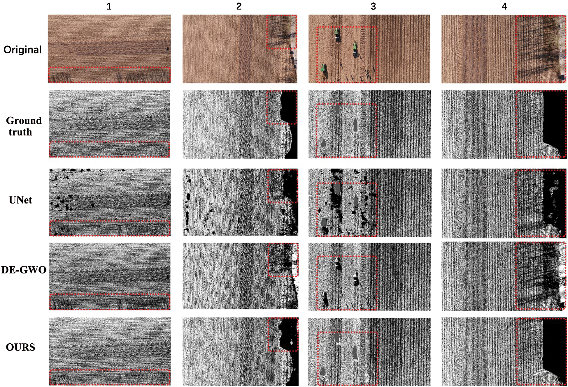
Figure 9: Detection results from farm with different complexity

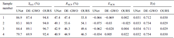
For the farmland under the above four complex scenarios, the experimental results obtained after using three different algorithms to segment the farmland are shown in Tab. 5. It can be seen that the IoU of straw for the algorithm proposed in this paper is the highest. In Sample 1, the straw IoU was improved by 7.9% and 7.4% compared with UNet and the traditional algorithm, respectively, and the coverage error was reduced to 0.002. In Sample 2, there were many mistakes for UNet, and so the straw IoU was only 83.1%. The traditional algorithm had a poor multi–class segmentation effect and the straw IoU was only 80.9%. Finally, the proposed algorithm can achieve a good segmentation and resulted in straw IoU of 94%. In Sample 3, the mIoU reached up to 96.7%, the straw coverage rate was 49.6%, and the straw coverage error reached the lowest because the algorithm in this paper could well segment the agricultural machinery and eliminate the interference from people and their shadows. The experimental verification showed that 40% of the segmented agricultural machinery area was straw. However, the traditional method cannot separate the agricultural machinery, and most is recognized as straw; therefore, the error was obvious. Sample 4 was complex farmland containing a large number of tree shadows, roads and vegetation. The algorithm proposed in this paper dealt with all of them well, and the straw IoU improved by 12.7% and 22.5% compared with UNet and the traditional algorithm, respectively. To sum up, the algorithm proposed in this paper can well conduct straw detection in complex scenes and segment straw when a large number of shadows from trees exist. Moreover, the running time for a 720 × 400 image is approximately 0.029 s, which means that it has obvious speed advantages over the traditional algorithm, and it meets the practical detection requirements for accuracy and speed.

Table 5: Comparison of results from different modules

5  Conclusions

This paper proposed a semantic segmentation method to solve the problem of straw segmentation in complex scenes. A new network architecture, the RADw–UNet network, was designed by improving the UNet algorithm. The standard convolutional residual block and depthwise convolutional residual block were used to construct the whole network to reduce the number of parameters and improve the network segmentation accuracy. In the training, the weighted cross entropy loss function was adopted to make the network pay more attention to difficult classification areas and improve the contribution rate of straw to the network. Furthermore, the comparison experiments of the basal framework and different modules were designed to further verify the effectiveness of the proposed algorithm. The mIoU was 94.9%, the number of parameters was only 0.26M, and the running speed was up to 34 frames per second when the algorithm was applied to straw segmentation; therefore, the effect was better than that of traditional segmentation based on a threshold or texture and other semantic segmentation networks.

Acknowledgement: Conceptualization, Y.L., S.Z. and Y.W.; methodology, S.Z. and Y.L.; software, S.Z. and H.F.; validation, Y.L., S.Z. and Y.W.; formal analysis, Y.L. and H.Y.; investigation, Y.L. and H.Y. ; data curation, Y.L. H.F., H.S. and X.Z.; writing—original draft preparation, S.Z., H.F. H.S. and X.Z.; writing—review and editing, Y.L., Y.W. and H.Y.; supervision, Y.W. and H.Y.

Funding Statement: This research was funded by National Natural Science Foundation of China, grant number 42001256, key science and technology projects of science and technology department of Jilin province, Grant Number 20180201014NY, science and technology project of education department of Jilin province, Grant Number JJKH20190927KJ, innovation fund project of Jilin provincial development and reform commission, Grant Number 2019C054.

Conflicts of Interest: The authors declare that they have no conflicts of interest to report regarding the present study.

References

This work is licensed under a Creative Commons Attribution 4.0 International License, which permits unrestricted use, distribution, and reproduction in any medium, provided the original work is properly cited.

References

1H. Yin, W. Zhao, T. Li, X. Cheng and Q. Liu. (2018), “Balancing straw returning and chemical fertilizers in China: Role of straw nutrient resources. ,” Renewable and Sustainable Energy Reviews, vol. 81, no. (2), pp, 2695–2702, .
2H. Zhang, J. Hu, Y. Qi, C. Li, J. Chen et al.. (2017). , “Emission characterization, environmental impact, and control measure of PM2. 5 emitted from agricultural crop residue burning in China. ,” Journal of Cleaner Production, vol. 149, pp, 629–635, .
3N. Hu, B. Wang, Z. Gu, B. Tao, Z. Zhang et al.. (2016). , “Effects of different straw returning modes on greenhouse gas emissions and crop yields in a rice-wheat rotation system. ,” Agriculture, Ecosystems & Environment, vol. 223, pp, 115–122, . [Google Scholar]
4L. Wang, L. Xu and S. Wei. (2017), “Straw coverage detection method based on sauvola and otsu segmentation algorithm. ,” Agricultural Engineering, vol. 7, pp, 29–35, . [Google Scholar]
5H. Li, H. Li and J. He. (2009), “Field coverage detection system of straw based on artificial neural network. ,” Transactions of the Chinese Society for Agricultural Machinery, vol. 40, pp, 58–62, . [Google Scholar]
6Y. Liu, Y. Wang and H. Yu. (2018), “Detection of straw coverage rate based on multi–threshold image segmentation algorithm. ,” Transactions of the Chinese Society for Agricultural Machinery, vol. 149, pp, 7–35, . [Google Scholar]
7A. Krizhevsky, I. Sutskever and G. E. Hinton. (2017), “Imagenet classification with deep convolutional neural networks. ,” Communications of the ACM, vol. 60, pp, 84–90, . [Google Scholar]
8K. Simonyan and A. Zisserman, “Very deep convolutional networks for large-scale image recognition. ,” arXiv preprint arXiv, 1409.1556. v6, pp. 1–14, 2015. [Google Scholar]
9A. Krizhevsky, I. Sutskever and G. E. Hinton. (2012), “Imagenet classification with deep convolutional neural networks. ,” in Proc. of the Int. Conf. on Neural Information Processing Systems 2012, Lake Tahoe, NV, USA: , pp, 1097–1105, .
10C. Szegedy, W. Liu, Y. Jia, P. Sermanet, S. Reed et al.. (2015). , “Going deeper with convolutions. ,” in Proc. of the IEEE Conf. on Computer Vision and Pattern Recognition, Boston, MA, USA: , pp, 1–9, .
11Y. J. Luo, J. H. Qin, X. Y. Xiang, Y. Tan, Q. Liu et al., “Coverless real-time image information hiding based on image block matching and dense convolutional network,” Journal of Real-Time Image Processing, vol. 17, no. 1, pp. 125–135, 2020.
12W. Wang, Y. T. Li, T. Zou, X. Wang, J. Y. You et al., “A novel image classification approach via dense-mobileNet models,” Mobile Information Systems, vol. 1, pp. 1–8, 2020.
13S. Ren, K. He, R. Girshick and J. Sun, “R-CNN: Towards real-time object detection with region proposal networks,” IEEE Transactions on Pattern Analysis and Machine Intelligence, vol. 39, pp. 1137–1149, 2017. [Google Scholar]
14J. Redmon, S. Divvala, R. Girshick and A. Farhadi, “You only look once: Unified, real-time object detection,” in Proc. of the IEEE Conf. on Computer Vision and Pattern Recognition 2016, Las Vegas, NV, USA, pp. 779–788, 2016. [Google Scholar]
15W. Liu, D. Anguelov, D. Erhan, C. Szegedy, S. Reed et al.. (2016). , “Single shot multibox detector. ,” in Proc. of the European Conf. on Computer Vision, Amsterdam, Holland: , pp, 21–37, .
16J. M. Zhang, X. K. Jin, J. Sun, J. Wang and A. K. Sangaiah. (2018), “Spatial and semantic convolutional features for robust visual object tracking. ,” Multimedia Tools and Applications, vol. 17, pp, 1–21, .
17D. Y. Zhang, Z. S. Liang, G. B. Yang, Q. G. Li, L. D. Li et al.. (2018). , “A robust forgery detection algorithm for object removal by exemplar-based image inpainting. ,” Multimedia Tools and Applications, vol. 77, no. (10), pp, 11823–11842, . [Google Scholar]
18E. Wang, Y. Jiang, Y. Li, J. Yang, M.Ren et al.. (2019). , “MFCSNet: Multi-scale deep features fusion and cost-sensitive loss function based segmentation network for remote sensing images. ,” Applied Sciences, vol. 9, no. (19), pp, 1–18, . [Google Scholar]
19S. Pereira, A. Pinto, V. Alves and C. A. Silva. (2016), “Brain tumor segmentation using convolutional neural networks in MRI images. ,” IEEE Transactions on Medical Imaging, vol. 35, no. (5), pp, 1240–1251, .
20B. Benjdira, A. Ammar, A. Koubaa and K. Ouni. (2020), “Data-efficient domain adaptation forsemantic segmentation of aerial imagery using Generative Adversarial Networks. ,” Applied Sciences, vol. 10, pp, 1–24, .
21D. Y. Zhang, Q. G. Li, G. B. Yang, L. D. Li and X. M. Sun. (2017), “Detection of image seam carving by using weber local descriptor and local binary patterns. ,” Journal of Information Security and Applications, vol. 36, pp, 135–144, .
22Y. T. Chen, J. J. Tao, L. Y. Liu, J. Xiong, R. L. Xia et al.. (2020). , “Research of improving semantic image segmentation based on a feature fusion model. ,” Journal of Ambient Intelligence and Humanized Computing, vol. 39, pp. 1137–1149, . [Google Scholar]
23L. Jonathan, S. Evan and D. Trevor. (2015), “Fully convolutional networks for semantic segmentation. ,” in Proc. of the IEEE Conf. on Computer Vision and Pattern Recognition, Boston, MA, USA: , pp. 3431–3440, . [Google Scholar]
24Y. Liu, S. Zhang, H. Yu, Y. Wang and J. Wang. (2020), “Straw detection algorithm based on semantic segmentation in complex farm scenarios. ,” Editorial Office of Optics and Precision Engineering, vol. 28, pp, 200–211, . [Google Scholar]
25O. Ronneberger, P. Fischer and T. Brox. (2015), “U-Net: Convolutional networks for biomedical image segmentation. ,” in Int. Conf. on Medical Image Computing and Computer–Assisted Intervention, Munich, Germany: , pp, 234–241, . [Google Scholar]
26K. He, X. Zhang, S. Ren and J. Sun. (2016), “Deep residual learning for image recognition. ,” in Proc. of the IEEE Conf. on Computer Vision and Pattern Recognition, Las Vegas, NV, USA: , pp, 770–778, . [Google Scholar]
27F. Chollet. (2017), “Xception: Deep learning with depthwise separable convolutions. ,” in Proc. of the IEEE Conf. on Computer Vision and Pattern Recognition, Hawaii, HL, USA: , pp, 1251–1258, . [Google Scholar]
28A. Vaswain, N. Shazeer and N. Parmar. (2017), “Attention is all you need. ,” Advances in Neural Information Processing Systems, vol. 1, pp, 5998–6008, . [Google Scholar]
29B. Zhao, X. Wu and J. Feng. (2017), “Diversified visual attention networks for fine–grained object classification. ,” IEEE Transactions on Multimedia, vol. 19, pp, 1245–1256, . [Google Scholar]
30M. Noori, A. Bahri and K. Mohammadi. (2019), “Attention-guided version of 2D UNet for automatic brain tumor segmentation. ,” in Int. Conf. on Computer and Knowledge Engineering, Mashhad, Iran: , pp, 269–275, . [Google Scholar]
31J. Fu, J. Liu, H. Tian, Y. Li, Y. Bao et al.. (2019). , “Dual attention network for scene segmentation. ,” in Proc. of the IEEE Conf. on Computer Vision and Pattern Recognition, Long Beach, CA, USA: , pp, 3146–3154, . [Google Scholar]
32H. Li, P. Xiong and J. An. “Pyramid attention network for semantic segmentation. ,” arXiv preprint arXiv: 1805.10180. v3, pp. 1–13, 2018. [Google Scholar]
33K. He, X. Zhang, S. Ren and J. Sun. (2016), “Identity mappings in deep residual networks. ,” in Proc. of the European conf. on Computer Vision, Amsterdam, Holland: , pp, 630–645, . [Google Scholar]
34G. H. Andrew, M. Zhu, B. Chen, K. Dmitry, W. Wang et al.. (2017). , “Mobilenets: Efficient convolutional neural networks for mobile vision applications. ,” arXiv preprint arXiv: 1704.04861. v1, pp. 1–9, . [Google Scholar]
35J. Hu, L. Shen and G. Sun. (2018), “Squeeze-and–excitation networks. ,” in Proc. of the IEEE Conf. on Computer Vision and Pattern Recognition, Salt Lake, UT, USA: , pp, 7132–7141, . [Google Scholar]
36V. Badrinarayanan, A. Kendall and R. Cipolla. (2017), “SegNet: A deep convolutional encoder-decoder architecture for image segmentation. ,” IEEE Transactions on Pattern Analysis and Machine Intelligence, vol. 39, no. (12), pp, 2481–2495, . [Google Scholar]
37C. Li, Y. Zhu and G. Papandreou. (2018), “Encoder-decoder with atrous separable convolution for semantic image segmentation. ,” in Proc. of the European Conf. on Computer Vision, Munich, Germany: , pp, 801–818, . [Google Scholar]