DOI:10.32604/cmc.2020.012380
| Computers, Materials & Continua DOI:10.32604/cmc.2020.012380 | |
| Article |
A Dynamically Reconfigurable Accelerator Design Using a Sparse-Winograd Decomposition Algorithm for CNNs
National University of Defence Technology, Changsha, China
*Corresponding Author: Jianzhuang Lu. Email: lujz1977@163.com
Received: 28 June 2020; Accepted: 25 July 2020
Abstract: Convolutional Neural Networks (CNNs) are widely used in many fields. Due to their high throughput and high level of computing characteristics, however, an increasing number of researchers are focusing on how to improve the computational efficiency, hardware utilization, or flexibility of CNN hardware accelerators. Accordingly, this paper proposes a dynamically reconfigurable accelerator architecture that implements a Sparse-Winograd F(2 × 2.3 × 3)-based high-parallelism hardware architecture. This approach not only eliminates the pre-calculation complexity associated with the Winograd algorithm, thereby reducing the difficulty of hardware implementation, but also greatly improves the flexibility of the hardware; as a result, the accelerator can realize the calculation of Conventional Convolution, Grouped Convolution (GCONV) or Depthwise Separable Convolution (DSC) using the same hardware architecture. Our experimental results show that the accelerator achieves a 3x–4.14x speedup compared with the designs that do not use the acceleration algorithm on VGG-16 and MobileNet V1. Moreover, compared with previous designs using the traditional Winograd algorithm, the accelerator design achieves 1.4x–1.8x speedup. At the same time, the efficiency of the multiplier improves by up to 142%.
Keywords: High performance computing; accelerator architecture; hardware
At present, CNNs are widely used in various fields impacting different areas of people’s lives, such as image classification [1], target recognition [2,3], semantic segmentation [4,5], and so on. However, with the development of CNNs, networks have become deeper and deeper, with some even reaching tens to hundreds of layers [6,7], introducing a huge workload to the system in terms of computing and storage. At the same time, due to the emergence of new convolution methods such as DSC and GCONV, the flexibility of CNN accelerators has become more and more important.
Many solutions have been proposed to solve the associated problems. These include using the Graphics Processing Units (GPUs) [8], Application Specific Integrated Circuits (ASICs) [9–12], Field-Programmable Gate Arrays (FPGA) [13–15] and other hardware to facilitate the acceleration of CNNs. However, GPUs are impacted by a high power consumption problem, while ASCIs are affected by high production costs and a long development, which greatly limits their scope of application.
As face recognition, motion tracking and other applications have become widely used in both mobile devices and embedded devices, the demand for CNNs in these devices is also increasing. Because embedded and mobile devices have more limited hardware resources and higher power consumption requirements, lightweight CNNs such as MobileNet [16,17], ShuffleNet [18], Xception [19] have been proposed one after another. However, due to the high computing and high throughput characteristics of CNNs, running even lightweight CNNs is also associated with huge challenges when it comes to improving on-chip computing performance, storage, bandwidth, and power consumption. At the same time, different CNNs or different convolutional layers usually have different convolution shapes, which also presents challenges to ensuring the flexibility of hardware accelerators. As a result, hardware architecture designers must improve data reusability and computing performance, reduce system operating power consumption, or reduce the bandwidth requirements. Moreover, such hardware must ensure that features are dynamically reconfigurable if it is to meet the system’s flexibility requirements when adapting to different lightweight CNNs.
This paper proposes a fast decomposition method based on the Sparse-Winograd algorithm (FDWA); this approach extends the applicability of the Winograd algorithm to various convolution shapes and further reduces the computational complexity. Based on unified hardware implementation, it is able to provide a high level of configurability, to realize fast switching between different configurations for different convolution shapes at runtime. Generally speaking, the main advantages of this architecture are as follows:
•Using the FDWA can not only reduce the number of multiplications and shorten the loop iteration of the convolution, but also introduces dynamic sparseness into the network; this can reduce hardware workload, improve the speed of convolution execution, expand the use scope of the Sparse-Winograd algorithm, and simplify the hardware implementation. Moreover, compared with the conventional accelerator design, the proposed hardware architecture design also enhances the adaptability and flexibility of the accelerator, meaning that the accelerator can accelerate both Conventional Convolutions and the new types of convolution (such as DSC or GCONV) without the need to change the hardware architecture.
•This paper proposes a high-throughput 2D computing architecture with reconfigurable I/O parallelism, which improves PE Array utilization. A linear buffer storage structure based on double buffers is used to reduce the data movement overhead between all levels of storage and to hide the data movement time, such that the computing performance of the entire system runs at the peak computing speed of the PE Array.
The remainder of this paper is organized as follows. The second section summarizes the related work. The third section briefly introduces the Winograd algorithm and outlines the operation of the FDWA in detail. Section 4 details the architecture of the accelerator, while Section 5 provides the implementation results and comparison. Finally, Section 6 presents the conclusion.
Previous studies have proposed a wide range of CNNs accelerator architectures. The DianNao [20,21] series achieved good end results by improving the parallel computing performance, enhancing the computing arrays, optimizing the data flow patterns, and increasing data reuse rates. Eyeriss [22] reduces data movement by maximizing local data reuse, applying data compression, implementing data gating, and achieving high energy efficiency. The Efficient Inference Engine (EIE) [23] introduces a sparse network to speed up the fully connected layer’s operation speed. Sparse CNN (SCNN) [24] accelerates the speed of convolution calculation under sparse network conditions by improving the coding and hardware structure. Zhang et al. [25] improve the convolution calculation by mapping the Fast Fourier transform (FFT) algorithm; for their part, Shen et al. [26] improve the computing speed of both 2D and 3D convolution by mapping the Winograd algorithm, thereby achieving good results on FPGA. The work of Wang et al. [27], based on the Fast Finite Impulse Response Algorithm (FFA), reduces the number of multiplication operations in the convolution operation; however, the flexibility of this design is so weak that it can only be accelerated for a fixed type of convolution. Lu et al. [28] designed an accelerator based on the fast Winograd algorithm, but primarily used F(6, 3) and F(7, 3) as the basic calculation unit. Due to the large number of parameters, the hardware accelerator in this case is required to use 16-bit fixed-point operands, along with more complex pre-calculations. Even so, however, very few accelerator designs for lightweight neural networks have been developed, although there are some designs for light-weight CNN acceleration or that aim to increase accelerator flexibility.
In this article, in order to speed up operation, save on hardware resources, and improve the calculation efficiency, we designed the FDWA as a basic hardware design based on the Sparse-Winograd algorithm. Moreover, we go on to test the algorithm acceleration effect and hardware resource consumption via SystemC [29].
Firstly, it is feasible in practical terms to accelerate CNNs at the algorithm level. Various advanced convolution algorithms have therefore been applied to accelerator design. Taking Winograd, FFT, and FFA algorithms as examples, these approaches reduce the number of multiplication operations by reducing the computational complexity, thereby further saving on resources. Compared with the FFT and FFA algorithms, the Winograd algorithm can achieve better results when the convolution kernel is smaller [8]. In this paper, our approach is to solve different types of volume integrals and use fixed Sparse-Winograd  for calculation; this not only simplifies the implementation, but also expands the application range of the Winograd algorithm.
Secondly, the speed of CNN updating has accelerated of late, and there are usually great differences between the different convolutional layers in CNNs, meaning that higher requirements are placed on the flexibility of the accelerator. However, most studies based on algorithm acceleration typically only support a specific and fixed convolution type. At the same time, lightweight CNNs such as MobileNet and ShuffleNet have seen widespread use on mobile devices or embedded platforms, thereby reducing both the number of parameters and the computational complexity; one example is MobileNetV1 [16], which achieves acceptable results with less than 50% of the MAC operations and parameters utilized by comparison methods. This was primarily made possible due to the use of new convolution methods in the MobileNetV1 structure, including Group Convolution (GCONV) and Depthwise Separable Convolution (DSC). Accordingly, there is an urgent need to solve the acceleration problem of the new convolution method when designing hardware accelerators. This paper therefore proposes a hardware architecture design for accelerating various types of CNNs based on FDWA; this approach solves the algorithm flexibility problem, thereby facilitating adaptation to different convolution types, and also solves the problem of the need to speed up the new type of convolution.
3 Algorithm Analysis, Mapping and Improvement
At present, there have been few studies on hardware accelerators for lightweight CNNs. While Bai et al. [30] and Zhao et al. [31] realized the acceleration of convolution calculations for lightweight CNNs on FPGA, the main drawback of these works is that the overall performance and flexibility remain insufficient. In light of this, the present paper proposes a block parallel computing method based on the Sparse-Winograd algorithm and a reconfigurable decomposition method for lightweight CNNs, which solves the problems associated with accelerating different convolution types.
CNNs are primarily composed of convolutional layers, Rectified Linear Units (ReLUs), pooling layers, fully connected layers, etc. Of these components, the convolution layer has made a major contribution to CNN operation; however, it also takes up most of the calculation time.
Following the emergence of lightweight CNNs, new convolution method have been widely used due to their outstanding advantages. DSC was first proposed in MobileNet V1, while GCONV first appeared in AlexNet. As shown in Tab. 1 [16], MobileNet achieves image recognition accuracy that is almost as high as, or even higher than, that of comparison methods, while still using fewer parameters and less calculations; this is achieved by means of DSC, which demonstrated its outstanding advantage on embedded platforms or mobile devices.
Table 1: Comparison of MobileNet with popular models
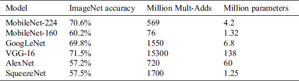
Fig. 1 presents the execution process of Conventional Convolution, GCONV and DSC. In particular, Fig. 1b describes the specific process of GCONV. This process involves dividing the input feature map into g groups according to the number of channels, such that the size of each input feature map group becomes 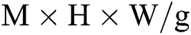 , while the size of the convolution kernel becomes
 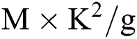 . During the execution process, the filter only performs convolution operations with input feature maps from the same group; in this way, it can reduce the number of parameters required during the convolution operation. Fig. 1c further describes the specific process of DSC. This process involves dividing the convolution process into two sub-processes: Depthwise Convolution and Pointwise Convolution. Firstly, each channel of the input feature map is independently convoluted via channel-by-channel convolution with a convolution kernel size of
 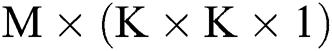 , after which it is deepened by point-by-point convolution. The weighted combination is then used to generate the output feature map, where the point-wise convolution kernel size is
 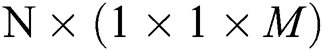 .
.
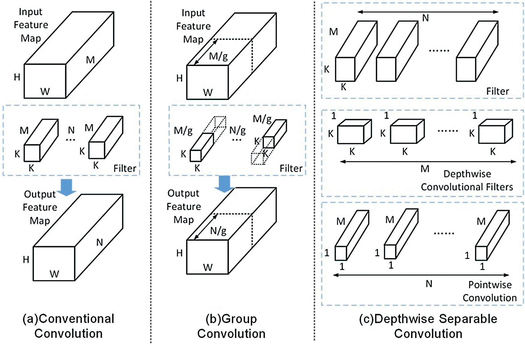
Figure 1: Conventional convolution, GCONV and DSC
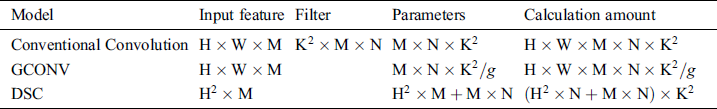
Tab. 2 specifically illustrates the difference in the number of parameters and the total amount of calculation for the three different convolution methods. Compared with Conventional Convolution, the new convolution method requires fewer resources and requires less external memory bandwidth requirements to achieve tolerable accuracy. Therefore, it is urgently necessary to develop a hardware architecture design hat can handle both Conventional Convolution and the new types of convolution.
Table 2: Parameter and calculation amount of different convolution methods
The Winograd algorithm is a new, fast algorithm for CNNs, which reduces the number of multiplication operations by transforming the input feature map and executing a series of transformations on the filter. Taking the one-dimensional Winograd algorithm as an example, the specific operation process can be expressed as follows:

In Eq. (1),  indicates the multiplication between corresponding elements. Moreover, A, B, and G are constant transformation coefficient matrices, which are determined by the size of the input data.
Similarly, the operation process of the 2D Winograd algorithm  can be described by Eq. (2). In summary, the input feature matrix X and the filter matrix W are converted into the Winograd domain by the matrices B and G, After the dot product operation is performed, the A matrix is used for transformation. The transformation matrices B, G, and A are determined by the size of the input feature map and the size of the filter.

It can be concluded from Eq. (2) that the 2D Winograd algorithm only needs to execute  multiplication operations, while
  operations are required for Conventional Convolution. Fig. 2 [28] describes the calculation process and pseudocode implementation of the convolution based on the 2D Winograd algorithm and Conventional 2D convolution; in this case, the convolution stride of the Winograd convolution algorithm is 1. It can be seen from observing at the the algorithm level that the Conventional Convolution method requires six layers of loops, while the Winograd algorithm-based convolution only requires four layers of loops and reduces the amount of necessary multiplication by more than 60% [28].
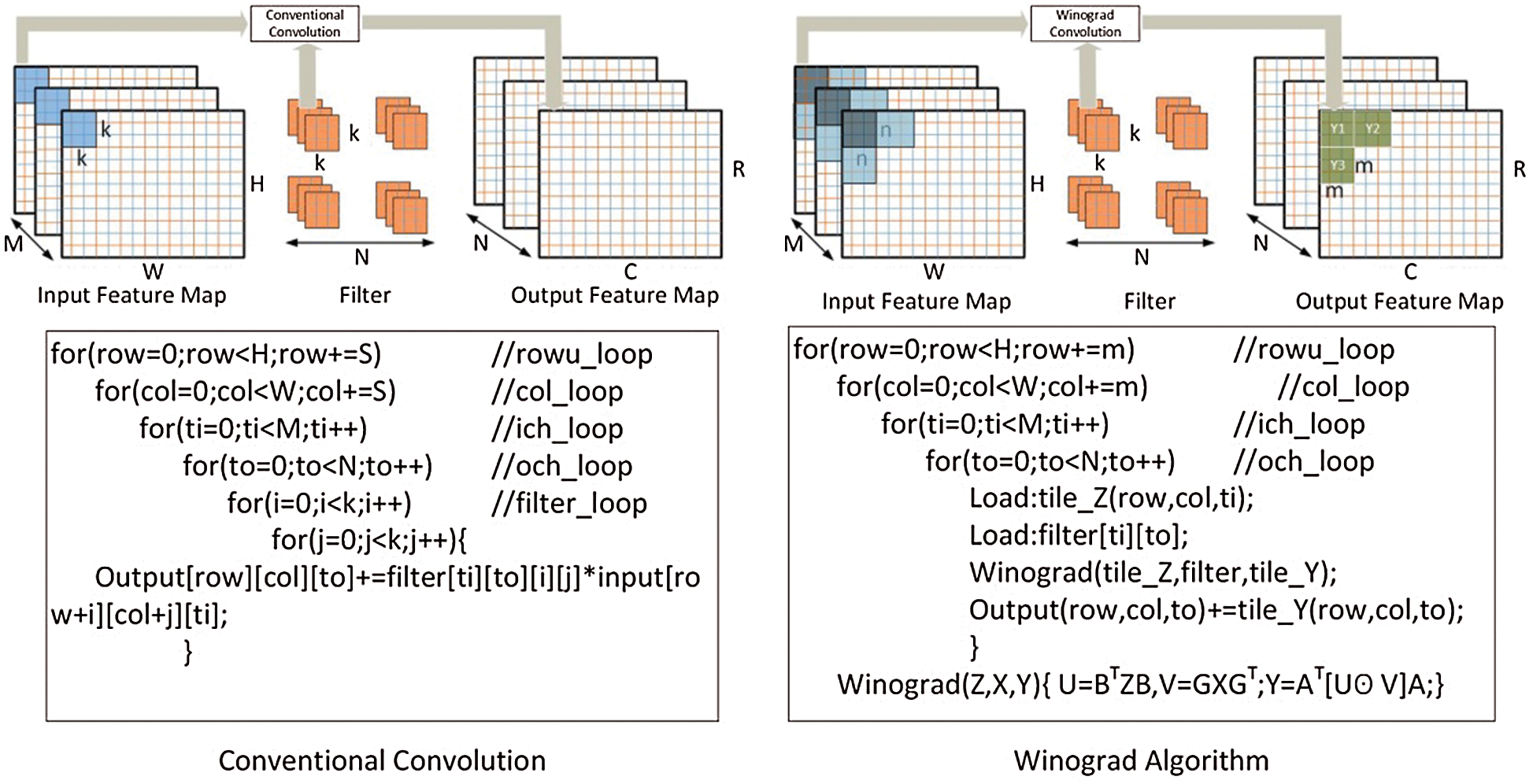
Figure 2: Comparison of conventional and Winograd convolution algorithms
By conducting further research into the Winograd algorithm, Liu et al. [32] and others proposed the Sparse-Winograd algorithm, based on the original algorithmic structure. As shown in Fig. 3 [32], there are different methods of applying the Winograd algorithm to a sparse network. The linear transformation of neurons and convolution kernels will reduce the sparsity of the original network. Therefore, if the Winograd algorithm is used to directly accelerate the sparse network, the number of multiplication operands in the network will increase, such that the ensuing performance loss will outweigh the benefit of using the Winograd acceleration algorithm.
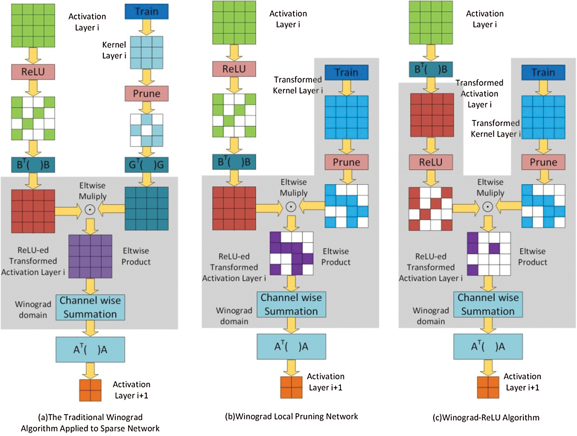
Figure 3: The Winograd algorithm applied to different sparse network situations
Fig. 3c describes the specific operation steps of the Sparse-Winograd algorithm in the case where  . Here, the ReLU activation function is moved to the Winograd domain, so that the CNNs are sparse during the multiplication operation, The number of multiplications is reduced, while the weights are pruned following the Winograd transform, meaning that the weights remain sparse during the multiplication operation. The algorithm can be expressed as follows:

By moving ReLU and Prune to the Winograd domain, the number of multiplication operations can be reduced, while the overall efficiency can be further improved when the Winograd algorithm is used for acceleration; thereby, the acceleration of a sparse network based on the Winograd algorithm can be realized.
3.3 Sparse-Winograd Algorithm Mapping and Improvement
Although convolution operations based on the Sparse-Winograd algorithm can reduce the number of required multiplication operations and improve the operational efficiency, for different types of convolutions, the operation process is overall the same as the Winograd algorithm but requires more complex pre-operations, primarily as regards the calculation of the conversion matrix A, B and G. Moreover, the calculation of the conversion matrix is also difficult to realize via hardware; in addition, with increases in size of the input feature map or the convolution kernel, the data range of the parameters in the conversion matrix becomes very large, which presents challenges for the design of hardware, storage, bandwidth, and power consumption. The above problems restrict the development of CNN accelerators based on the Sparse-Winograd algorithm.
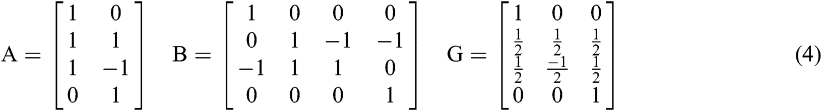
In order to solve the above problems, we propose a method of FDWA based on the Sparse-Winograd algorithm, which operated by decomposing the input feature map and filter on the basis of the Sparse-Winograd  algorithm. As shown in Eq. (4), the decomposition is based on
  and chiefly considers that the parameters in the transformation matrices A, B and G are
  . This is easy to achieve by shifting or adding hardware; not only is this hardware implementation simple and easy to control, but it also reduces the hardware cost.
Fig. 4 describes the process of  , where the Conventional Convolution steps after the input feature map and the filter are expanded by 0, along with the meaning of the parameter representation. Accordingly,
 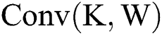 can be expressed by Eq. (5); moreover, Eqs. (6) to (9) outline the methods by which specific parameters are calculated.
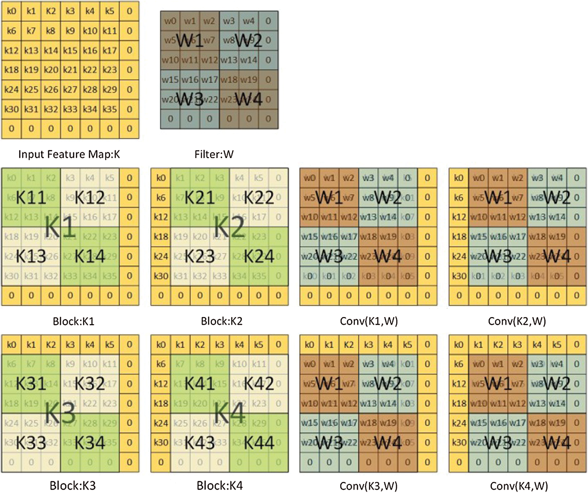
Figure 4: Explanation of parameters in the conventional convolution process
Fig. 5 describes the FDWA process in detail, with 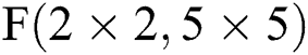 as an example. As shown in the figure, firstly, the input feature map and the filter are expanded to 7 × 7 and 6 × 6 scaled by zero, after which the four corner 4 × 4 scale blocks on the feature map (K1, K2, K3, K4) are respectively convoluted with the four 3 × 3 scale blocks(W1, W2, W3, W4) on the convolution kernel; subsequently, the
  can be calculated by a set of
  . Eqs. (10) to (13) describe each
  calculation result and the significance of the corresponding figures.
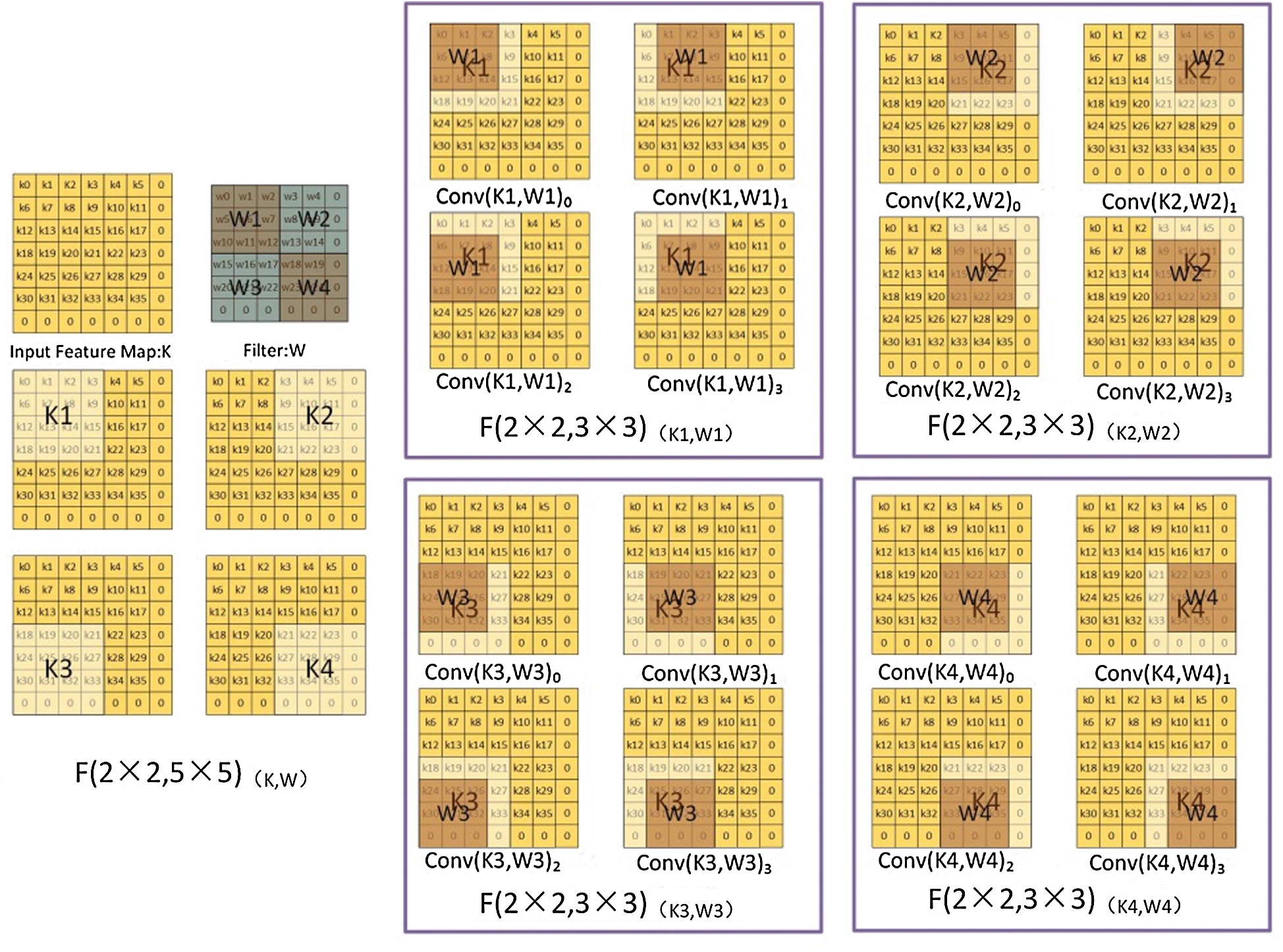
Figure 5: FDWA


As shown in Tab. 3, the parameters are equivalent to Eqs. (6) to (9) and Eqs. (10) to (13). From Tab. 3, we can also get the final process of the  calculation based on
  in Fig. 6.
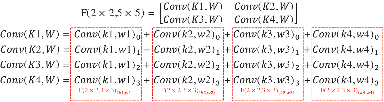
Figure 6: Decomposition calculation method of 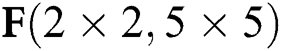
Table 3: Relationships between parameters for convention l and new convolutions
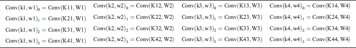
Fig. 7 describes three situations based on the above FDWA, specifically for  and
and  . As can be seen from Fig. 7b, the FDWA with filter size of 6 × 6 is the same as that of
  ; i.e., the filter size is between 3 and 6, while the partition method is the same. Fig. 7c describes the FDWA process in the case of
 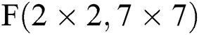 , which is also applicable to filter sizes between 7 and 9. When utilizing FDWA, it is easy to realize the accelerator design with
  as the hardware core. This design is not only simple to control, but also requires less pre-operation, expanding applicability and reducing hardware consumption.
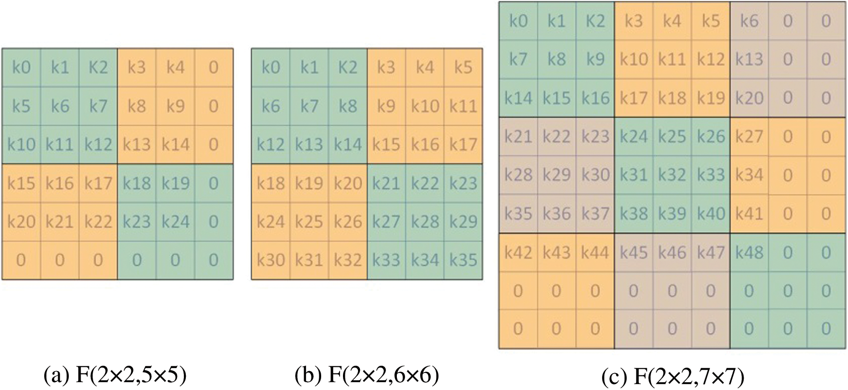
Figure 7: Decomposition calculation method of  and
and 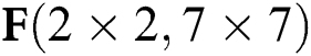
4 Accelerator Architecture Design
In this chapter, the accelerator scheme will be comprehensively introduced.
4.1 Overview of Accelerator Design
Fig. 8 illustrates the system-level architecture of the accelerator. The key components of the three modules are the processor, DRAM, Processing Units, and system interconnection bus.
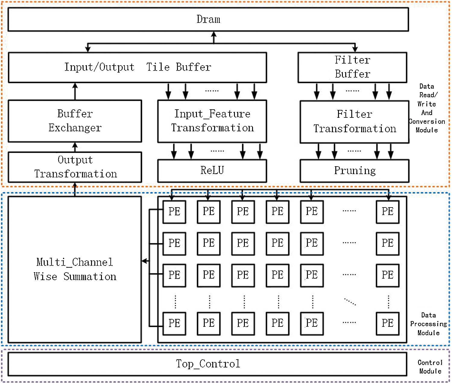
Figure 8: The structure overview of accelerator
1) Control module: This component is responsible for receiving the task information sent by the CPU. When the task is loaded on to the accelerator and calculations begin, the module will distribute the task to the calculation module, and prompt the DMA module to ei ther move the data to the buffer or write to the external DDR through the interconnection configuration. After calculation is complete, the module will move the result to the external DRAM and notify the CPU.
2) Data read (write) and conversion module: The input feature tile data is read from the buffer, after which the input is transferred to the Winograd domain through the input conversion module via the implementation of 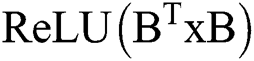 . The filter data is read from the external memory by the filter buffer. Conversion to the Winograd domain is then completed by performing
 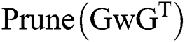 . Because these two data conversion processes only involve changes to symbol bits and shift operations, the calculation module does not need to be too complex. After the data operation is completed, the
  operation is executed to transform the resulting data into a 2 × 2 convolution; after the configurable accumulator operation, the expired data is finally overwritten in the input characteristic graph buffer and written back to the external memory.
3) Data calculation module: After conversion to the Winograd domain, the data input operation module completes the point product operation, after which the data flows to the accumulation module. In terms of the process of performing the accumulation operation, the information from the controller is received, and GCONV and DSC are completed by separating the channels. In the Sub-Channel operation of DSC, the data from all input channels are converted directly and then saved to the on-chip buffer. For GCONV, moreover the input channels are divided into several groups, after which the data in each group is aggregated and stored in the on-chip buffer following conversion.
4.2 Structural Design of Computing Module
The calculation module is used to process the converted data of the input feature map and filter. Fig. 9 illustrates the overall architecture design of the calculation module, which can be further divided into two main calculation sub-modules—namely, the Multi_Channel Wise Summation and Multiplication Calculation Array modules—that respectively complete the calculation of the accumulation and dot product by configuring different accumulator functions, and can thereby achieve the calculation of the DSC, GCONV, and Conventional Convolution.
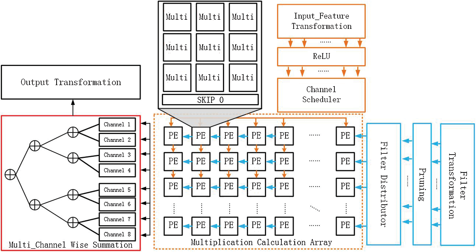
Figure 9: The architecture of the computing module
In the multiplication calculation array module, since the accelerator uses FDWA based on  , its core calculation is the dot product calculation between two matrices of size 4 × 4. Since the Sparse-Winograd algorithm introduces a lot of sparsity into the point product calculation, the point product calculation of the 4 × 4 matrices can be realized with fewer multipliers. Thus, in this design, 3 × 3 multipliers are used to realize the 2D dot product calculation; that is, 9 multipliers are designed in the PE. This is mainly because both the input feature block and the convolution kernel block are converted to ReLU and Prune respectively following the Winograd domain conversion. The overall density of the original parameters will decrease by about 40% to 50%. Therefore, it is reasonable to choose 9 multipliers. This meets most of the multiplication requirements in one cycle. Of course, there are certain (albeit very few) cases in which the multiplication operation needs to be greater than 9. When this occurs, two more cycles are required to pause a single PE pipeline. The dot product calculation unit in the entire calculation module is composed of 8 × 8 such PEs; this means that 64
  calculations can be performed simultaneously. In order to efficiently and accurately realize FDWA, after the input data is converted to the Winograd domain, a highly efficient and effective parallel operation module can be realized by inputting the feature map channel selector and the filter data distributor.
The input data is calculated and output by means of a dot product calculation module to a specific configurable accumulator for processing purposes. Through the setting of different multi-channel accumulator functions, the convolution acceleration calculation of the lightweight CNNs can be realized; this process also ensures the configurability of the accelerator.
As shown in Eq. (4), the parameters in the conversion matrix based on  only have
  ; thus, the multiplication and division operations can be replaced by shift, addition and subtraction operations, which reduces the computational complexity and saves on hardware resources. Fig. 10a presents the conversion template of the conversion matrix B, while Fig. 10b outlines the conversion template of the conversion matrix B; the combination of the two is the conversion module of the input feature block. Similarly, transformation matrices A and G, along with their transposition matrices, can also be used to obtain transformation templates consiing of addition, subtraction and shift.
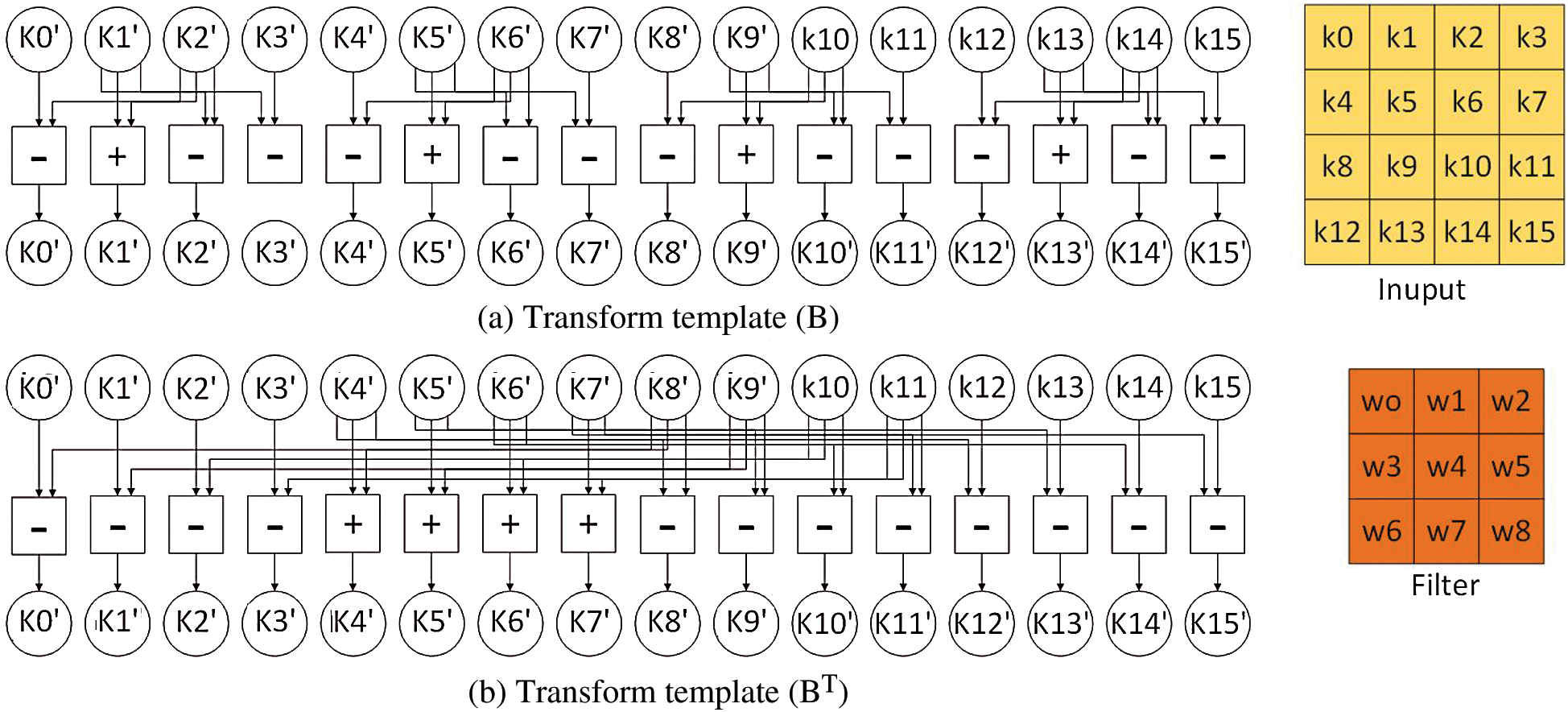
Figure 10: Conversion template of the conversion Matrix B
Since the on-chip storage space is insufficient to store the entire input feature map and filter, a specific storage structure is required if we are to improve the degree of data reuse and improve the smooth data transfer between storage structures at all levels. Fig. 11 illustrates the linear buffer module used in this design. For the input feature map  , there is only a low correlation between the data of each channel. After tiling is complete, the horizontal linear buffer contains M × W elements. In the buffer zone, after the input feature map has been divided into tiles according to the block algorithm, the Winograd domain conversion module completes the conversion and inputs the result into the PE to perform the calculation. Moreover, in order to improve the calculation efficiency, the data handling time is hidden in the data calculation. The input feature map buffer further adopts a ‘double buffer’ setting; that is, when the slider slides in m linear buffers, the other m linear buffers are ready for the next calculation. In the convolution kernel buffer, the convolution kernel is independently decomposed according to each channel of the decomposition method, while the Sparse-Winograd algorithm is executed on the subsequent input feature block.
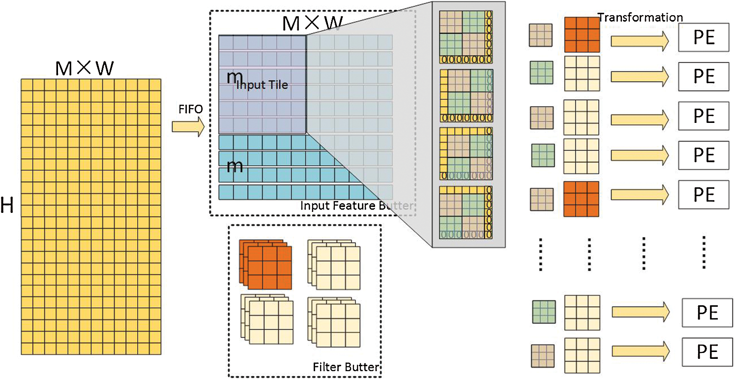
Figure 11: Storage architecture overview
5 Experimental Analysis and Results
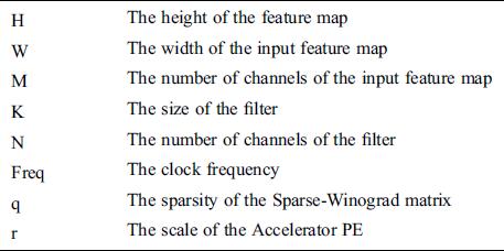
In this section, an analysis model will be established to help with theoretical analysis of the accelerator performance. Tab. 4 presents the meaning of each parameter expression.
Table 4: The meaning of each parameter
In theory, the total number of multiplication ( ) operations performed by a single-layer convolution in the accelerator design scheme can be calculated by Eq. (14), as follows:

The data throughput of the entire accelerator in a single cycle is  data points; thus, the required clock cycle can be expressed as follows:

Furthermore, the time required for the whole accelerator to run a single-layer convolution  can be expressed as follows:

SystemC is a collaborative software/hardware design language, as well as a new system-level modeling language. It contains a series of C++ classes and macros, and further provides an event-driven simulation core enabling the system designer to use C++ morphology in order to simulate parallel processes. In this paper, system C is used to accurately simulate each module and thread to facilitate counting of the number of cycles under a specific load. In order to fully consider the accelerator’s acceleration effect under various convolution conditions, this paper utilizes workloads that are typically representative of both Conventional Convolution and new convolution applications, which are named VGG-16 and MobileNet v1 respectively. The architecture parameters of each network are listed in Tab. 5. Each layer of DSC consists of DSC and SC, while the number of output channels is the convolution kernel size of SC, i.e.,  .
.
Table 5: The network architecture parameters of VGG-16 (left) and MobileNetV1 (right)
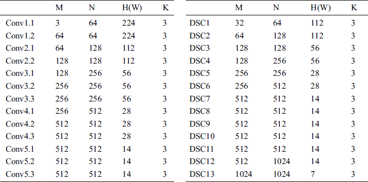
The first layer of the network, as the original input, does not pass through either the ReLU layer or the Prune layer, and its parameter density is 100%. In the simulation process, the accelerator operating frequency is set to 200 MHz, while the data itself is represented by 8-bit fixed points. Fig. 12 plots the running time after hardware implementation based on Conventional Convolution (in blue), the Winograd algorithm (in red), the Sparse-Winograd algorithm (in green), and FDWA (purple) under VGG-16. It can be seen from the figure that the dynamic sparseness introduced by the Sparse-Winograd algorithm both reduces the hardware workload and improves the execution speed. The Sparse-Winograd algorithm and FDWA achieve the fastest running times; accordingly, it can be seen that FDWA does not significantly reduce the running speed in exchange for improving the hardware applicability and reducing the hardware consumption. However, it should be noted that the FDWA is slow in the first layer of convolution operations; this is mainly due to the insufficient sparsity of the first layer of convolution parameters, which results in the interruption of pipelines and an increased number of empty and other cycles.
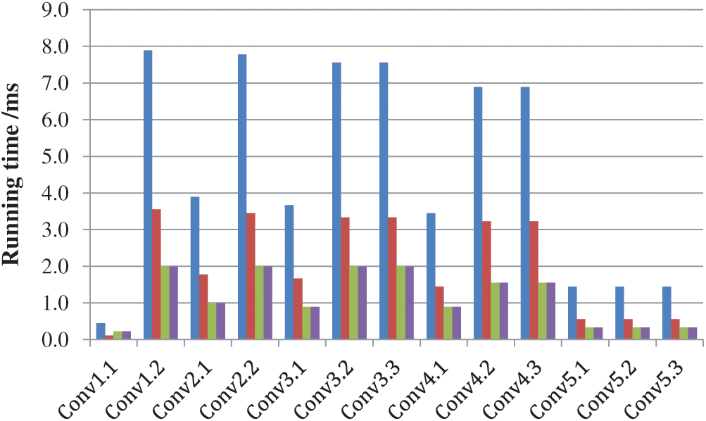
Figure 12: Running time of VGG-16 under different convolution methods
Moreover, Fig. 13 plots the running time after hardware implementation based on deep separable convolution (in blue), the Winograd acceleration algorithm (in red), Sparse-Winograd acceleration algorithm (in green), and FDWA (in purple) under the MobileNet V1 load. The figure shows us that the Sparse-Winograd acceleration algorithm and FDWA can still obtain a very good acceleration effect. However, as MobileNet V1 subsequently performs DSC, although the input image size decreases due to the large number of channels, the number of convolutional layer operations also increases due to the increase in accelerator control time and storage time, resulting in an overall increase in total operation time.
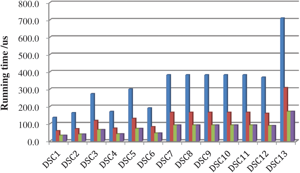
Figure 13: Running time of MobileNet V1 under different convolution methods
From the comparative analysis of Figs. 12 and 13, it can be seen that MobileNet V1 requires a shorter running time than the traditional VGG-16, which demonstrates the advantages of the new convolution method, as well as showing that the lightweight neural network is more suitable for embedded or mobile devices. It should however be noted that the actual running time of both is longer than the theoretical derivation time. This is mainly due to the fact that it is not possible to hide the time spent on system initialization, pipeline suspension, and data handling. However, for both Mobilenet V1 or VGG-16, it can be seen that the FDWA has an acceleration effect of 3x–4.15x, and further achieves an improvement of between 1.4x–1.8x compared with the traditional Winograd algorithm. Moreover, an accelerator that utilizes the FDWA has unparalleled advantages in terms of hardware flexibility: it is not only compatible with different convolution methods, but also capable to being adapted to different types of convolution sizes.
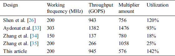
Tab. 6 presents a comparison between the design scheme of this paper and several mainstream accelerator design schemes, with a particular focus on the difference in hardware resource consumption and utilization rate. From the table, it can be concluded that the accelerator design scheme proposed in this paper not only resolves the issue of the accelerator being insufficiently applicable, but also exhibits a great advantage in terms of its utilization of hardware resources; this is mainly due to the dynamic sparsity brought about by the Sparse-Winograd algorithm and the skip 0 module in the calculation module, which reduce the amount of multiplication required, save on hardware consumption and improve the hardware (particularly multiplier) utilization.
Table 6: Hardware utilization of different design schemes
Based on the Sparse-Winograd algorithm, a highly parallel design of a reconfigurable CNN accelerator based on Sparse-Winograd  is realized in this paper. Our proposed model not only improves the applicability of the algorithm, but also avoids the complex pre-operation generally associated with Winograd series algorithms and reduces the difficulty of hardware implementation. After experimental verification, it can be concluded that the Sparse-Winograd algorithm decomposition method not only improves the operational efficiency of the algorithm in terms of hardware, but also realizes an acceleration of 3x–4.15x for VGG-16 and MobileNet V1, which is 1.4x–1.8x better than the Winograd algorithm.
Funding Statement: This paper and research results were supported by the Hunan Provincial Science and Technology Plan Project. The specific grant number is 2018XK2102. Yunping Zhao, Jianzhuang Lu and Xiaowen Chen all received this grant.
Conflicts of Interest: The authors declare that they have no conflicts of interest to report regarding the present study.
References
1A. Krizhevsky, I. Sutskever and G. E. Hinton. (2012), “ImageNet classification with deep convolutional neural networks. ,” in Proc. of Advances In Neural Information Processing Systems, pp, 1097–1105, .
2K. He, X. Zhang, S. Ren and J. Sun. (2016), “Deep residual learning for image recognition. ,” in Proc. of IEEE CVPR, pp, 770–778, . [Google Scholar]
3J. R. R. Uijlings, K. E. A. van de Sande, T. Gevers and A. W. M. Smeulders. (2013), “Selective search for object recognition. ,” International Journal of Computer Vision, vol. 104, no. (2), pp, 154–171, . [Google Scholar]
4R. Girshick, J. Donahue, T. Darrell and J. Malik. (2014), “Rich feature hierarchies for accurate object detection and semantic segmentation. ,” in Proc. of IEEE CVPR, pp, 580–587, . [Google Scholar]
5H. Noh, S. Hong and B. Han. (2015), “Learning deconvolution net-work for semantic segmentation. ,” in Proc. of IEEE ICCV, pp, 1520–1528, . [Google Scholar]
6A. Mollahosseini, D. Chan and M. H. Mahoor. (2016), “Going deeper in facial expression recognition using deep neural networks. ,” in Proc. of IEEE WACV, pp, 1–10, . [Google Scholar]
7H. Nakahara and T. Sasao. (2015), “A deep convolutional neural network based on nested residue number system. ,” in Proc. of IEEE FPL, pp, 1–6, . [Google Scholar]
8A. Lavin and S. Gray. (2016), “Fast algorithms for convolutional neural networks. ,” in Proc. of IEEE CVPR, pp, 4013–4021, . [Google Scholar]
9Y. H. Chen, T. Krishna, J. S. Emer and V. Sze. (2017), “Eyeriss: An energy-efficient reconfigurable accelerator for deep convolutional neural networks. ,” IEEE Journal of Solid-State Circuits, vol. 52, no. (1), pp, 127–138, . [Google Scholar]
10S. Yin. (2018), “A high energy efficient reconfigurable hybrid neural network processor for deep learning applications. ,” IEEE Journal of Solid-State Circuits, vol. 53, no. (4), pp, 968–982, .
11G. Desoli. (2017), “A 2.9TOPS/W deep convolutional neural network SoC in FD-SOI 28 nm for intelligent embedded systems. ,” in IEEE Int. Solid-State Circuits Conf. DigTech, pp, 238–239, .
12D. Shin, J. Lee, J. Lee and H. J. Yoo. (2017), “DNPU: An 8.1TOPS/W reconfigurable CNN-RNN processor for general-purpose deep neural networks. ,” in IEEE Int. Solid-State Circuits Conf. DigTech, pp, 240–241, . [Google Scholar]
13J. Wang, J. Lin and Z. Wang. (2018), “Efficient hardware architectures for deep convolutional neural network. ,” IEEE Transactions on Circuits and Systems I: Regular Papers, vol. 65, no. (6), pp, 1941–1953, . [Google Scholar]
14Y. Ma, Y. Cao, S. Vrudhula and J. S. Seo. (2018), “Optimizing the convolution operation to accelerate deep neural networks on FPGA. ,” IEEE Transactions on Very Large Scale Integration Systems, vol. 26, no. (7), pp, 1354–1367, .
15A. Ardakani, C. Condo, M. Ahmadi and W. J. Gross. (2018), “An architecture to accelerate convolution in deep neural networks. ,” IEEE Transactions on Very Large Scale Integration Systems, vol. 65, no. (4), pp, 1349–1362, . [Google Scholar]
16A. G. Howard, M. L. Zhu and B. Chen. Apr., 2017, “MobileNets: Efficient convolutional neural networks for mobile vision applications. ,” Computer Science, [Online]. Available: https://arxiv.org/abs/1704.04861?context=cs. [Google Scholar]
17M. Sandler, A. Howard and M. Zhu. (2018), “MobileNetV2: Inverted residuals and linear bottlenecks. ,” in The IEEE Conf. on Computer Vision and Pattern Recognition, pp, 4510–4520, . [Google Scholar]
18X. Y. Zhang, X. Y. Zhou, M. X. Lin and J. Su. (2018), “ShuffleNet: An extremely efficient convolutional neural network for mobile devices. ,” in The IEEE Conf. on Computer Vision and Pattern Recognition, pp, 6848–6856, . [Google Scholar]
19F. Chollet. (2017), “Xception: Deep learning with depthwise separable convolutions. ,” in The IEEE Conf. on Computer Vision and Pattern Recognition, pp, 1251–1258, . [Google Scholar]
20T. Chen, Z. Du and N. Sun. (2014), “DianNao: A small-footprint high-throuhput accelerator for ubiquitous machine-learning, ” in ACM SIGPLAN Notices, pp, 269–284, . [Google Scholar]
21Y. Chen, T. Lou and S. Liu. (2014), “DaDianNao: A machine-learning supercomputer. ,” in ACM Int. Sym. on Microarchitecture, pp, 609–622, . [Google Scholar]
22Y. H. Chen, T. Krishna, J. S. Emer and V. Sze. (2017), “Eyeriss: An energy-efficient reconfigurable accelerator for deep convolutional neural net-works. ,” IEEE Journal of Solid-State Circuits, vol. 52, no. (1), pp, 127–138, . [Google Scholar]
23S. Han, X. Liu and H. Mao. (2016), “EIE: Efficient inference engine on compressed deep neural network,” in ACM SIGARCH Computer Architecture News, pp, 243–254, . [Google Scholar]
24A. Parashar, M. Rhu and A. Mukkara. (2017), “SCNN: An accelerator for compressed-sparse convolutional neural networks. ,” in IEEE Int. Sym. on Computer Architecture, pp, 27–40, . [Online]. Available: https://dl.acm.org/doi/abs/10.1145/3140659.3080254. [Google Scholar]
25C. Zhang and V. Prasanna. (2017), “Frequency domain acceleration of convolutional neural networks on CPU-FPGA shared memory system. ,” in Proc. of ACM. SIGDA Int. Sym. on Field-Programmable Gate Arrays, pp, 35–44, [Online]. Available: https://dl.acm.org/doi/abs/10.1145/3020078.3021727. [Google Scholar]
26J. Z. Shen, Y. Huang and Z. Wang. (2018), “Towards a uniform template-based architecture for accelerating 2D And 3D CNNs on FPGA. ,” in Proc. of ACM. SIGDA Int. Sym. on Field-Programmable Gate Arrays, pp, 97–106, . [Online]. Available: https://dl.acm.org/doi/abs/10.1145/3174243.3174257. [Google Scholar]
27J. Wang, J. Lin and Z. Wang. (2018), “Efficient hardware architectures for deep convolutional neural network. ,” IEEE Transactions on Circuits and Systems I: Regular Papers, vol. 65, no. (6), pp, 1941–1953, . [Google Scholar]
28L. Lu, Y. Liang, Q. Xiao and S. Y. An. (2017), “Evaluating fast algorithms for convolutional neural networks on FPGAs. ,” in Proc. of IEEE FCCM, pp, 101–108, . [Google Scholar]
29Q. Zhang, Y. Li and M. Sun. (2019), “Automatic generation of systemC code from mediator. ,” in Computer Engineering and Science, pp, 835–842, . [Google Scholar]
30L. Bai, Y. Zhao and X. Huang. (2018), “A CNN accelerator on FPGA using depthwise separable convolution. ,” IEEE Transactions on Circuits and Systems II-Express Briefs, vol. 65, no. (10), pp, 1415–1419, . [Google Scholar]
31R. Zhao, X. Niu and W. Luk. (2018), “Automatic optimising CNN with depth-wise separable convolution on FPGA. ,” in Proc. of ACM/SIGDA FPGA, pp, 285, . [Google Scholar]
32X. Liu, J. Pool, S. Han and W. J. Dally. (2018), “Efficient Sparse-Winograd convolutional neural networks. ,” ICLR, [Google Scholar]
33U. Aydonat, S. O’Connell, D. Capitali and C. L. Andrew. (2017), “An OpenCL deep learning accelerator on Arria10. ,” in SIGDA Int. Sym. on Field-Programmable Gate Arrays, pp, 55–64, . [Online]. Available: https://dl.acm.org/doi/abs/10.1145/3020078.3021738.
34C. Zhang, P. Li, G. Sun, Y. Guan and B. Xiao. (2015), “Optimizing FPGA-based accelerator design for deep convolutional neural works. ,” in SIGDDA Int. Sym. on Field-Programmable Gate Arrays, pp, 161–170, . [Online]. Available: https://dl.acm.org/doi/abs/10.1145/2684746.2689060.
35C. Zhang, Z. Fang, P. Zhou, P. Peichen and C. Jason. (2016), “Caffeine: Towards uniformed representation and acceleration for deep convolutional neural networks. ,” in ACM Int. Conf. on Computer-Aided Design, no. 12, .
 | This work is licensed under a Creative Commons Attribution 4.0 International License, which permits unrestricted use, distribution, and reproduction in any medium, provided the original work is properly cited. |