DOI:10.32604/cmc.2020.012869
| Computers, Materials & Continua DOI:10.32604/cmc.2020.012869 | |
| Article |
Resampling Factor Estimation via Dual-Stream Convolutional Neural Network
1School of Data and Computer Science, Guangdong Province Key Laboratory of Information Security Technology, Ministry of Education Key Laboratory of Machine Intelligence and Advanced Computing, Sun Yat-sen University, Guangzhou, 510006, China
2Academy of Forensic Science, Shanghai, 200063, China
3College of Information Science and Technology, Jinan University, Guangzhou, 510632, China
4Department of Computer Science, University of Massachusetts Lowell, Lowell, MA 01854, USA
*Corresponding Author: Wei Lu. Email: luwei3@mail.sysu.edu.cn
Received: 15 July 2020; Accepted: 28 August 2020
Abstract: The estimation of image resampling factors is an important problem in image forensics. Among all the resampling factor estimation methods, spectrum-based methods are one of the most widely used methods and have attracted a lot of research interest. However, because of inherent ambiguity, spectrum-based methods fail to discriminate upscale and downscale operations without any prior information. In general, the application of resampling leaves detectable traces in both spatial domain and frequency domain of a resampled image. Firstly, the resampling process will introduce correlations between neighboring pixels. In this case, a set of periodic pixels that are correlated to their neighbors can be found in a resampled image. Secondly, the resampled image has distinct and strong peaks on spectrum while the spectrum of original image has no clear peaks. Hence, in this paper, we propose a dual-stream convolutional neural network for image resampling factors estimation. One of the two streams is gray stream whose purpose is to extract resampling traces features directly from the rescaled images. The other is frequency stream that discovers the differences of spectrum between rescaled and original images. The features from two streams are then fused to construct a feature representation including the resampling traces left in spatial and frequency domain, which is later fed into softmax layer for resampling factor estimation. Experimental results show that the proposed method is effective on resampling factor estimation and outperforms some CNN-based methods.
Keywords: Image forensics; image resampling detection; parameter estimation; convolutional neural network
Nowadays, with the emergence of convenient and easy-to-use image processing software, non-experts can easily edit and manipulate digital images without leaving obvious perceptible artifacts, which degrades the authority of digital images as an evidence for criminal investigation and legal proceedings. Besides the changes of the image content, some illegal information could be embedded in a digital image [1,2]. Although tampered images usually maintain high visual quality, image manipulation generally destroys inherent statistical consistency of tampered images and leaves unique traces. In last two decades, digital image forensics techniques have attracted substantial research interest including image information security [3], image forensics [4,5], image deblurring [6] and image steganalysis [7].
As a common post-processing part of many manipulations, geometric transformations such as scaling are widely used to make forgers more realistic, introducing notable resampling traces. Therefore, resampling detection has drawn more and more attention. A great deal of analysis about resampling detection and parameter estimation have been proposed in the last two decades. Despite the diversity of approaches, most of the existing detectors share a common processing framework, which can be summarized in two steps. First of all, a residual signal from the observed image is extracted for detecting resampling artifacts. Depending on different foundation of each method, this residual signal can be obtained by calculating the variance of the difference of the observed image [8], by filtering the image with a linear filter [9] or by calculating the normalized energy density for different window sizes of images [10]. Secondly, by exposing the traces hiding in the residual signal, a decision on whether resampling operation has been applied on the observed image can be rendered. Some approaches apply a post-processing in the frequency domain to detect the spectral peaks induced by resampling process [11]. On the contrary, some methods avoid the post-processing part and check if the pixel and its neighbors satisfy the underlying linear structure [12]. Besides, some methods make good use of Support Vector Machine (SVM) to make the final decision instead of analyzing the traces in frequency or space domain. For example, Wang et al. [13] calculate the singular value decomposition of the observed image as the features to train the SVM. More related works can be found in [14–17]. Among all the resampling detection methods, spectrum-based method [18–21] is one of the most widely used approach which is capable of resampling factor estimation as well. However, a weakness of spectrum-based methods is ambiguity which greatly influences the accuracy of factor estimation. According to Gallagher [8], a spectral peak in the spectrum of an image is corresponding to three resampling factors. Most of existing spectrum-based methods limit their research on particular region such as downscaling factor estimation or upscaling factor estimation.
Stimulated by the progress that deep learning has brought to the computer vision [22–24], convolutional neural networks (CNNs) are widely applied in the field of digital image forensics [25–27]. Instead of directly feed the investigated images into a network, many of the current deep learning based approaches for forensics prefer to pre-process the images by a set of filters for content suppression [28], by extracting residual images [29,30] or by computing several transformation domain representations like DCT coefficients [31,32]. Besides, some CNN based methods tend to adjust the network architecture for better performance on detection. For example, a novel type of convolutional layer, called constrained convolutional layer, has been proposed for image forgery detection task [33,34]. Instead of using pre-trained models, this approach adaptively extracts image manipulation features by forcing CNN to learn prediction-error filters. In addition, a CNN-based architecture for resampling parameter estimation is proposed [35], which analyses the sensitivities to mismatch between training and testing data points to failure cases. Moreover, Cao et al. [36] proposed a dual-stream CNN to capture the resampling trails along different directions. They concatenate the horizontal and vertical streams to construct more powerful feature representative for resampling detection and resampling region location.
In this paper, we propose a dual-stream resampling parameter estimation framework which comprises of gray steam and frequency stream. An input image is first transformed into frequency domain to obtain its spectrum. Later, the image itself is directly fed into gray stream and its spectrum is fed into frequency stream to extract high dimension features, respectively. Features from these two streams are then concatenated to construct finally feature representative which includes the resampling traces left in space and frequency domain. The frequency stream is used for suppressing the influence of image contents to obtain better description of resampling. Our experiment results show the effectiveness of the proposed method in detecting both upscaled and downscaled factor.
The remainder of the paper is organized as follows. In Section 2, we present a review of prior work on resampling forensics. In Section 3, we elaborate the architecture of the proposed resampling parameter estimation network. In Section 4, extensive experimental results and analysis are included. In Section 5, the conclusions are summarized.
To maintain the authenticity of tampered image content, it is often necessary to perform geometric manipulations like scaling and rotation, which introduce resampling and interpolation. At its core, resampling maps the pixels of the original image from its source coordinates to a new coordinates of the resampled image. However, the size of the resampled image generally does not align with the original image. An interpolation step is thus involved to calculate the value of the pixels that only occurs in the resampled image. Most of the image interpolation kernels in practical are linearly separable. Without loss of generality, we consider rescaling a signal with scaling factor  in one dimension, which maps pixels
  from source signal
  to a new sampling location to obtain the resampled signal

as a result of linear interpolation with kernel  . In this case, factor
  imply upscaling and
  denote downscaling.
Most resampling detectors expose the existence of resampling operation by exploiting periodic traces in resampled signals. Popescu et al. [12] found that the resampling process introduces correlations between neighboring samples to some extent. In this case, a set of periodic samples that are correlated to their neighbors can be found in resampled signals, and the period length of the specific statistical correlations depends on the scaling factor. They employed expectation maximization (EM) algorithm to estimate probability maps which exposes the periodic patterns hidden in resampled images. Their method was later improved by Kirchner [9] with a fixed local linear predictor, which is more effective with higher accuracy.
Compared to the method that directly exposes the periodic patterns of resampled images, Gallagher [8] proposed a simple and fast approach to detect resampling operation and estimate its scaling factor. He first computed the second derivative of the resampled images

where  is an operator of the 2nd order derivative. He also found that the variance of the second order derivative of a resampled image has a periodicity equal to the scaling factor

where  is an integer and
  means variance process. Later, this theory had been extended to kth derivative by Mahdian et al. [11]. In a word, resampled images and their derivatives have inherent periodicity and its period corresponds to resampling factor.
After extracting the periodical signal from the resampled images by derivatives or linear predictor residues, a post-processing is then applied in the frequency domain to determine the existence of resampling operation. In the frequency domain, the spectral peaks are related to the period of periodical signal which means the presence of spectral peaks is a sign of resampling. Fig. 1 shows the 1-D FFT and 2-D FFT of an original image and its up-scaled version with a factor of 1.5. As we can see, the resampled image has two distinct and strong peaks in 1-D FFT and four prominent peaks in 2-D FFT, while the spectrum of original image has no clear peaks. It is observed that the original image and resampled image differ in frequency domain.
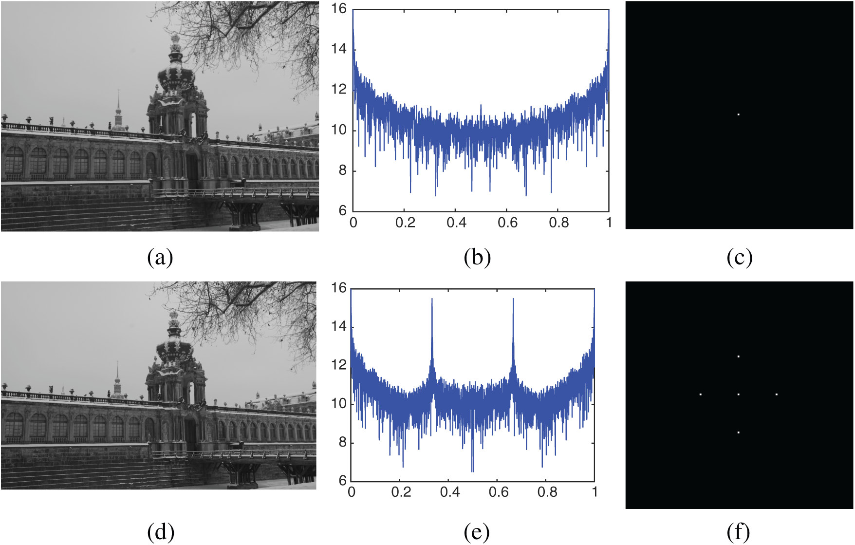
Figure 1: The 1-D FFT and 2-D FFT of an original image and its resampled version with a factor of 1.5. (a) Original image. (b) 1D-FFT of (a). (c) 2D-FFT of (a). (d) Upscale (a) with  . (e) 1-D FFT of (d). (f) 2-D FFT of (d)
In addition, the spectral peaks are related to the resampling parameter according to Gallagher. The link between spectral peaks and resampling parameter can be used for resampling factor estimation. Because of aliasing, several scaling factor may correspond to the same frequency peaks. Despite this unavoidably ambiguity, the estimated scaling factor  can be calculated as follows
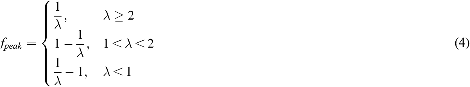
where  denotes the frequency of spectral peaks.
In recent years, it has been shown that deep neural networks are capable of extracting complex statistical dependencies and widely applied in the field of digital forensics. Bayar et al. [27] proposed constrained convolutional layer for resampling detection and resampling factor estimation. They used constrained convolutional layer to suppress an image’s content and adaptively learn manipulation detection features. This network architecture achieves high performance in manipulation detection including resampling detection. It is worth to note that CNN based resampling approaches [34–36] are capable of discriminating up-scaling and down-scaling, overcoming the ambiguity of spectrum-based methods.
In this section, we give an overview of dual-stream CNN architecture for resampling parameter estimation. Fig. 2 depicts the overall design of our proposed dual-stream CNN architecture. It consists of four main components. Firstly, in order to capture different dimensional features, the spectrum of the investigated image is computed to be fed into frequency stream and the investigated image itself is sent into gray stream. Secondly, the high level representation of image manipulation features is generated by gray and frequency streams. Thirdly, features of gray and frequency streams are concatenated to construct comprehensive representation of resampling traces. Finally, the concatenated features are fed into the softmax layer which is used for multiple classification. A detailed introduction of such four components are presented below.
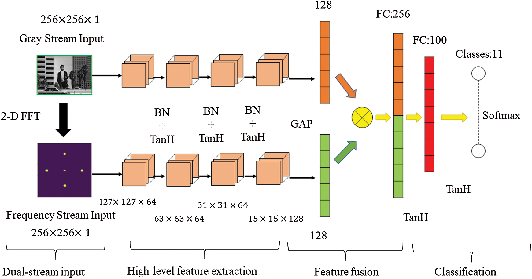
Figure 2: Proposed dual-stream CNN architecture. BN means batch normalization. TanH means hyperbolic tangent layer. GAP means global average pooling. FC means fully connected layer
To better characterize the resampling images, several features are adopted to model richer tampering artifacts. In our network architecture, we use a dual-stream network to learn rich features for resampling parameter identification, which contains gray stream and frequency stream. The input of gray stream is resampled image itself without any post-process. Each input has dimension of  . With the help of subsequent convolutional layers, the gray stream is designed to capture characteristic long-ranging correlation patterns between neighboring pixels, learning feature representation of resampling traces left in spatial domain. In the meanwhile, the frequency stream receives the spectrum of the investigated image and learns feature representation of resampling traces left in frequency domain. As discussed in Section 2, the spectrum of resampled images have prominent peaks which do not occur in un-resampled images. Hence, the input of frequency stream suppresses the image content and provides detectable features for training CNN.
3.2 High Level Feature Extraction
In our second conceptual block, we use a set of regular convolutional layers to learn new associations and higher-level prediction-error features. As shown in Fig. 2, the size of all convolutional kernels is  . We can also notice that all convolutional layers are followed by a batch normalization (BN) layer. Specifically, this type of layer minimizes the internal covariate shift, which changes the input distribution of a learning system by applying a zero-mean and unit-variance transformation of the data when training the CNN model. All the BN layers are followed by a nonlinear mapping called activation function. This type of function is applied to each value in the feature maps of every convolutional layer. In our CNN, we use TanH activation layer, which is one of the widely used activation in CNN architecture.
The output of the last convolutional layer of previous step is then fed into global average pooling (GAP) to generate a feature representation of gray and frequency stream. GAP is an operation that calculates the average output of each feature map in the previous layer. This simple operation reduces the data size significantly and prepares for the final classification component. It also has no trainable parameters because GAP just compute the average of each feature map. Each element of the feature representation corresponds to one feature map of the previous convolutional layer. In this case, the feature map is more closely related to the classification categories. Compared to use fully connected layer to generate feature representation, the use of GAP removes a large number of trainable parameters from the model and hence speeds up the training process, reducing the tendency of over-fitting. Moreover, due to the averaging operation over the feature maps, the model is more robust to spatial translations. After the feature representation of gray and frequency stream is given, both feature representation will be concatenated together to generate the concatenated feature which contains resampling traces left in spatial and frequency domain introduced by resampling operation.
To identify the resampling parameter that an input image has undergone, the concatenated feature is fed to a classification block which consists of a fully-connected neural network defined by three layers. More specifically, the first two fully-connected layers contain 256 and 100 neurons respectively. These layers learn new association between the deepest convolutional features in CNN. The output layer, also called classification layer, contains eleven neurons for each possible resampling parameter. Fully-connected layers resemble a feature space transformation which transforms high feature space to low feature space. It is beneficial for extracting the dominant features in previous high dimensional feature space and debasing the influence of noise. Through such a classification layer, the probability corresponding to each category is obtained and the most probable category is the output of the network.
In this section, extensive experiments are conducted to verify the performance of the proposed method. We implemented the proposed network using Pytorch framework and trained it on a machine equipped with a NVIDIA GTX 1070. All the experiments are carried out on a PC with Intel(R) Core(TM) i7 (2.80 GHz) processer, and 16G memory, running the Windows 10 operating system.
For a quantitative evaluation, we used 1000 uncompressed images ( ) captured by different Nikon cameras from the Dresden image database [37], which had been created for digital image forensics. Each original image was converted to grayscale and then non-overlapping divided into sub-images with the size of
  . We took 20,000 patches from it to create our un-resampling dataset. The images were respectively sampled with eleven different scaling factors in the range of [0.5,
  , 1.5] using three interpolation kernels, i.e., bilinear, bicubic and lanczos2. In total, we created a set of 660,000 images. Among them, we used 440,000 images for training network and the rest were used as our test dataset. The network trained used the Adam optimizer with random parameter initialization. The learning rate is 0.001 and the weight decay is 0.9.
4.2 Effectiveness Validation of Dual-Stream
In order to assess the performance of gray stream and frequency stream, three cases (using gray stream, frequency stream, and dual-stream) are studied respectively. As is shown in Fig. 3, the accuracies of gray stream and frequency stream models are 97.09% and 95.45% on average, respectively. Due to aliasing, the performance of frequency stream worse than gray stream. Meanwhile, the accuracy of the dual-stream model is 98.42%, which is the most effective model among three models. It can be seen clearly that the accuracy of the two one-stream methods are lower than the dual-stream method. The primary reason is that only one dimension feature is considered in one-stream method. However, different features play different roles on resampling parameter estimation. For example, the frequency stream is beneficial for suppressing image content while the gray stream contributes to learn the periodic pattern introduced by resampling. Thus, when both the gray and frequency features are taken into account, the accuracy rate will gain 1% improvement. On the basis of the obtained outcomes, it is obvious that the proposed dual-stream architecture could improve the performance for resampling parameter estimation.
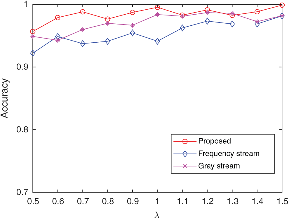
Figure 3: Scaling factor estimation accuracy for three input schemes: proposed dual-stream, only frequency stream and only gray stream
4.3 Comparison with Existing Algorithms
In this experiment, an analysis of the performance comparison between two CNN-based methods [34,35] and one spectrum-based method [8] is given. To present the performance comprehensively, we take the Mean Absolute Error (MAE) as performance criterion [19,35]. The performance for varying resampling factors using different interpolation kernels is shown in Tab. 1, with the best results highlighted in bold. As we can see, four resampling factor estimation methods achieve better performance in the images with lanczos2 interpolation kernel compared to bilinear and bicubic interpolation kernel. This is because the value of the interpolated pixels in resampled images takes most of neighboring pixels in original images into consideration when using lanczos2 as interpolation kernels. In this case, the pixels of resampled image become more closely linked to each other so that the period pattern introduced by resampling becomes more pronounced. In other words, the better the interpolation kernel is used, the better estimation accuracy can be rendered.
Table 1: Performance in terms of the MAE for scaling estimation with different scaled factor estimation methods. The investigated images are scaled with a factor of  with three interpolation kernel
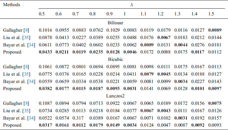
Experiments show that the MAE of our proposed scheme are less than 0.05 for all tested resampling factors. Typically, it can achieve less than 0.015 on upscaling factors for all the three interpolation kernels. The performance of our proposed scheme on upscaling factor estimation is similar to the other three competing methods which demonstrates the ability of the proposed scheme on upscaling factor estimation. However, the MAE of the other three methods increase in the case of downscaling factor estimation. On the contrary, although the MAE of the proposed scheme still increase for downscaling factor estimation, the MAE increment is the smallest compared to the other three methods. For example, the MAE of Liu et al. [35] increases 0.011 compared with upscaling factor 1.1 and downscaling factor 0.9 using lanczos2 as interpolation kernel. And, in the same case, Bayar et al. [34], Gallagher [8] increases 0.0096 and 0.085, respectively. While the MAE of the proposed scheme only increases 0.002. In general, it is very challenging to extract resampling traces in downscaled images since downscaling operation may result in loss of information about pixel value relationships. That is why the performance of all the resampling factor estimation methods decrease on downscaling factor estimation. However, the proposed scheme maintains pretty good performance on downscaling factor estimation. This is because the frequency stream used in our proposed architecture. The input of the frequency stream is the spectrum of investigated images which does not depend on the pixel relationships between neighbors, extracting the resampling traces in frequency domain for resampling factor estimation. Specifically, the MAE of the proposed scheme on estimating downscaled images with a factor of 0.5 is closed to 0.03, superior to other methods. This result demonstrates that the proposed scheme works with a relatively stable performance on scaling factor estimation.
In practice, we have no prior knowledge about which interpolation kernels is used in a resampled image. Therefore, for further accessing the performance of each resampling factor estimation methods, the accuracy is also considered in our experiment. Fig. 4 shows the accuracy of different methods on resampling factor estimation averaging with three interpolation kernels. As we can see, the proposed method achieves accuracy over 90% for different resampling factor of the test dataset, which means the proposed scheme has significant classification performance. It can be observed that four methods achieve high classification performance in upscaling factor estimation. However, the accuracy of the other three competing methods degrades in downscaling factor estimation. This is because the relationships of most of the pixel value are destroyed after an image is being downscaled which weakens the period pattern in spatial domain introduced by resampling. On the contrary, the proposed scheme maintains high classification accuracy for downscaling factors. Since the frequency stream of the proposed scheme receives the spectrum of investigated images and suppresses image content, the proposed scheme can still detect the resampling traces in frequent domain when estimates downscaling factors and maintains high classification accuracy.

Figure 4: Scaling factor estimation accuracy averaging with three interpolation kernels
In this paper, we presented a new CNN-based architecture for resampling factor estimation. A dual-stream CNN architecture is proposed to extract resampling features from both spatial domain and frequency domain. The gray stream aims at exposing the periodical patterns left in spatial domain introduced by resampling operation. Meanwhile, the frequency domain suppresses the image content and concentrates on spectral peaks which are beneficial for exposing the difference between original images and resampled images. The experimental results demonstrate that an end-to-end network design is capable of estimating rescaling factors accuracy, with mean absolute estimation errors well below some existing resampling factor estimation methods. Besides, the proposed network has the ability to discriminate upscale and downscale factor, overcoming the inherently ambiguity of spectrum-based methods. In the future, we would extend our work to detect the presence of resampling and estimate resampling parameters in the existence of more complex operation chain.
Funding Statement: This work is supported by the National Natural Science Foundation of China (No. 62072480), the Key Areas R&D Program of Guangdong (No. 2019B010136002), the Key Scientific Research Program of Guangzhou (No. 201804020068).
Conflicts of Interest: The authors declare that they have no conflicts of interest to report regarding the present study.
References
1. W. Su, X. Wang and Y. Shen. (2019). “Reversible data hiding based on pixel-value-ordering and pixel block merging strategy,” Computers, Materials & Continua, vol. 59, no. 3, pp. 925–941.
2. Q. Mo, H. Yao, F. Cao, Z. Chang and C. Qin. (2019). “Reversible data hiding in encrypted image based on block classification permutation,” Computers, Materials & Continua, vol. 59, no. 1, pp. 119–133.
3. J. Zhang, W. Lu, X. Yin, W. Liu and Y. Yeung. (2019). “Binary image steganography based on joint distortion measurement,” Journal of Visual Communication and Image Representation, vol. 58, pp. 600–605.
4. M. Lu, S. Niu and Z. Gao. (2020). “An efficient detection approach of content aware image resizing,” Computers, Materials & Continua, vol. 64, no. 2, pp. 887–907.
5. Z. Shen, F. Ding and Y. Shi. (2020). “Digital forensics for recoloring via convolutional neural network,” Computers, Materials & Continua, vol. 62, no. 1, pp. 1–16.
6. H. Xiao, W. Lu, R. Li, N. Zhong, Y. Yeung et al. (2019). , “Defocus blur detection based on multiscale SVD fusion in gradient domain,” Journal of Visual Communication and Image Representation, vol. 59, pp. 52–61.
7. J. Chen, W. Lu, Y. Yeung, Y. Xue, X. Liu et al. (2018). , “Binary image steganalysis based on distortion level co-occurrence matrix,” Computers, Materials & Continua, vol. 55, no. 2, pp. 201–211.
8. A. C. Gallagher. (2005). “Detection of linear and cubic interpolation in JPEG compressed images,” in Canadian Conf. on Computer and Robot Vision, Victoria, BC, Canada, pp. 65–72.
9. M. Kirchner. (2008). “Fast and reliable resampling detection by spectral analysis of fixed linear predictor residue,” in ACM Workshop on Multimedia and Securit, Oxford, UK, pp. 11–20.
10. X. Feng, I. J. Cox and G. Doerr. (2012). “Normalized energy density-based forensic detection of resampled images,” IEEE Transactions on Multimedia, vol. 14, no. 3, pp. 536–545.
11. B. Mahdian and S. Saic. (2008). “Blind authentication using periodic properties of interpolation,” IEEE Transactions on Information Forensics and Security, vol. 3, no. 3, pp. 529–538.
12. A. C. Popescu and H. Farid. (2005). “Exposing digital forgeries by detecting traces of resampling,” IEEE Transactions on Signal Processing, vol. 53, no. 2, pp. 758–767.
13. R. Wang and X. Ping. (2009). “Detection of resampling based on singular value decomposition,” in Int. Conf. on Image and Graphics, Xi’an, Shanxi, China, pp. 879–884.
14. D. Vázquez-Padín, C. Mosquera and F. Pérez-González. (2010). “Two-dimensional statistical test for the presence of almost cyclostationarity on images,” in Int. Conf. on Image Processing, HK, China, pp. 1745–1748.
15. D. Vázquez-Padín and P. Comesaña. (2012). “ML estimation of the resampling factor,” in Int. Workshop on Information Forensics and Security, Tenerife, Spain, pp. 205–210.
16. D. Vázquez-Padín, P. Comesaña and F. Pérez-González. (2015). “An SVD approach to forensic image resampling detection,” in European Signal Processing Conf., Nice, France, pp. 2067–2071.
17. D. Vázquez-Padín, F. Pérez-González and P. Comesaña. (2017). “A random matrix approach to the forensic analysis of upscaled images,” IEEE Transactions on Information Forensics and Security, vol. 12, no. 9, pp. 2115–2130.
18. Q. Zhang, W. Lu, T. Huang, S. Luo, Z. Xu et al. (2020). , “On the robustness of JPEG post-compression to resampling factor estimation,” Signal Processing, vol. 168, pp. 107371.
19. X. Liu, W. Lu, Q. Zhang, J. Huang and Y. Shi. (2019). “Downscaling factor estimation on pre-JPEG compressed images,” IEEE Transactions on Circuits and Systems for Video Technology, vol. 30, no. 3, pp. 618–631.
20. M. Kirchner and T. Gloe. (2009). “On resampling detection in re-compressed images,” in IEEE Int. Workshop on Information Forensics and Security, London, UK, pp. 21–25.
21. C. Chen, J. Ni, Z. Shen and Y. Q. Shi. (2017). “Blind forensics of successive geometric transformations in digital images using spectral method: Theory and applications,” IEEE Transactions on Image Processing, vol. 26, no. 6, pp. 2811–2824.
22. K. He, X. Zhang, S. Ren and J. Sun. (2016). “Deep residual learning for image recognition,” in Computer Vision and Pattern Recognition, Las Vegas, Nevada, USA, pp. 770–778.
23. A. Krizhevsky, I. Sutskever and G. E. Hinton. (2012). “ImageNet classification with deep convolutional neural networks,” in Neural Information Processing Systems, Lake Tahoe, Nevada, USA, pp. 1097–1105.
24. K. Simonyan and A. Zisserman. (2014). “Very deep convolutional networks for large-scale image recognition,” in Computer Vision and Pattern Recognition, Columbus, Ohio, USA.
25. Z. Shen, D. Feng and Y. Shi. (2019). “Digital forensics for recoloring via convolutional neural network,” Computers, Materials & Continua, vol. 62, no. 1, pp. 1–16.
26. J. Chen, X. Kang, Y. Liu and J. Wang. (2015). “Median filtering forensics based on convolutional neural networks,” IEEE Signal Processing Letters, vol. 22, no. 11, pp. 1849–1853.
27. B. Bayar and M. C. Stamm. (2018). “Constrained convolutional neural networks: A new approach towards general purpose image manipulation detection,” IEEE Transactions on Information Forensics and Security, vol. 13, no. 11, pp. 2691–2706.
28. Y. Rao and J. Ni. (2016). “A deep learning approach to detection of splicing and copy-move forgeries in images,” in Int. Workshop on Information Forensics and Security, Abu Dhabi, UAE, pp. 1–6.
29. D. Cozzolino and L. Verdoliva. (2016). “Single-image splicing localization through autoencoder-based anomaly detection,” in Int. Workshop on Information Forensics and Security, Abu Dhabi, UAE, pp. 1–6.
30. P. Zhou, X. Han, V. I. Morariu and L. S. Davis. (2018). “Learning rich features for image manipulation detection,” in Computer Vision and Pattern Recognition, Salt Lake City, Utah, USA, pp. 1053–1061.
31. V. Verma, N. Agarwal and N. Khanna. (2018). “DCT-domain deep convolutional neural networks for multiple JPEG compression classification” Signal Processing-Image Communication, vol. 67, no. 3, pp. 22–33.
32. Q. Wang and R. Zhang. (2016). “Double JPEG compression forensics based on a convolutional neural network,” Eurasip Journal on Information Security, vol. 2016, no. 1, pp. 5.
33. B. Bayar and M. C. Stamm. (2017). “On the robustness of constrained convolutional neural networks to JPEG post-compression for image resampling detection,” in IEEE Int. Conf. on Acoustics, Speech and Signal Processing, New Orleans, LA, USA, pp. 2152–2156.
34. B. Bayar and C. S. Matthew. (2017). “A generic approach towards image manipulation parameter estimation using convolutional neural networks,” in Information Hiding, Philadelphia, PA, USA, pp. 147–157.
35. C. Liu and M. Kirchner. (2019). “CNN-based rescaling factor estimation,” in The ACM Workshop, Princeton, New Jersey, USA, pp. 119–124.
36. G. Cao, A. Zhou, X. Huang, G. Song, L. Yang et al. (2019). , “Resampling detection of recompressed images via dual-stream convolutional neural network,” Mathematical Biosciences and Engineering, vol. 16, no. 5, pp. 5022.
37. T. Gloe and R. Bohme. (2010). “The `Dresden image database’ for benchmarking digital image forensics,” in ACM Sym. on Applied Computing, Sierre, Switzerland, vol. 2, pp. 1584–1590.
 | This work is licensed under a Creative Commons Attribution 4.0 International License, which permits unrestricted use, distribution, and reproduction in any medium, provided the original work is properly cited. |