DOI:10.32604/cmc.2020.012070
| Computers, Materials & Continua DOI:10.32604/cmc.2020.012070 | |
| Article |
An Effective Numerical Method for the Solution of a Stochastic Coronavirus (2019-nCovid) Pandemic Model
1Department of Mathematics and General Courses, Prince Sultan University Riyadh, Riyadh, Saudi Arabia
2Department of Medical Research, China Medical University Hospital, China Medical University, Taichung, 40402, Taiwan
3Department of Mathematics, Hashemite University, Zarqa, Jordan
4Stochastic Analysis & Optimization Research Group, Department of Mathematics, Air University, PAF Complex E-9, Islamabad, 44000, Pakistan
5Department of Mathematics, National College of Business Administration and Economics, Lahore, Pakistan
6Faculty of Engineering, University of Central Punjab, Lahore, 54500, Pakistan
7Department of Mathematics, Comsats University, Islamabad, Pakistan
*Corresponding Author: Ali Raza. Email: Alimustasamcheema@gmail.com
Received: 12 June 2020; Accepted: 07 August 2020
Abstract: Nonlinear stochastic modeling plays a significant role in disciplines such as psychology, finance, physical sciences, engineering, econometrics, and biological sciences. Dynamical consistency, positivity, and boundedness are fundamental properties of stochastic modeling. A stochastic coronavirus model is studied with techniques of transition probabilities and parametric perturbation. Well-known explicit methods such as Euler Maruyama, stochastic Euler, and stochastic Runge–Kutta are investigated for the stochastic model. Regrettably, the above essential properties are not restored by existing methods. Hence, there is a need to construct essential properties preserving the computational method. The non-standard approach of finite difference is examined to maintain the above basic features of the stochastic model. The comparison of the results of deterministic and stochastic models is also presented. Our proposed efficient computational method well preserves the essential properties of the model. Comparison and convergence analyses of the method are presented.
Keywords: Coronavirus pandemic model; stochastic ordinary differential equations; numerical methods; convergence analysis
Chen et al. [1] described the novel COVID-19 as a respiratory disease spread through droplets from the coughs, sneezes, or saliva of an infected person. The symptoms of this disease include fever, fatigue, suffocation, dry cough, and dyspnea. A human-made disease, xenophobia, spreads because of the violation of cohabitation law in Africa and other parts of the world. The concept of nationality has broken the unity of humanity and made people forget that this fractious world is a part of nature. Every mortal person is just a passenger. Lin et al. [2] stated that the concept had created inequalities, and racism had led to the false interaction of human beings, and ultimately the violation of natural law and the spread of fatal, sexually-transmitted diseases. Kucharski et al. [3] proposed that the environment does not grant permission for individuals to perform sexual activity with every person present, and neither does it allow them to eat whatever they want. Nature offers them some fruits, vegetables, and seafood; however, some items exist that are prohibited by nature, and likewise for human interactions with other beings. There are living beings that require no contact with humans. This mode of contact may be lethal and lead to the transmission of diseases like HIV, from chimpanzees to humans. HIV before the 1980s was a disease whose transmission was unknown, and whose symptoms were invisible [4]. Ebola is an example of human interaction with a non-human primate, a fruit bat that threatens a significant loss of life. Shereen et al. [5] clarified that it is assumed that Lassa fever develops from a rat, another example of false human contact. Humans have developed techniques to eliminate the deleterious effects of false interactions, but also fail. The COVID-19 pandemic is a prominent example of this failure. This virus has taken the lives of many individuals around the world. It is often called Wuhan COVID-19 because it originated in this town, which is the capital of Hubei in China. Zhao et al. [6] said that this virus was first transmitted to humans through a non-human source, and then transmitted quickly between humans, proving deadly. Symptoms of this disease may include a dry cough along with fever, and it may affect the respiratory tract by destroying the lungs. Tahir et al. [7] described this virus as a causative agent of a new disease identified as COVID-19, comprised of pneumonia followed by severe respiratory disorders. Much laboratory research has been conducted in China since December 2019 to sequence this virus. The World Health Organization (WHO) first classified it as SARS-CoV-2, before naming it COVID-19. After February, the epidemic became a pandemic causing numerous deaths in countries such as Italy, France, Germany, the UK, the USA, and Iran, which could not withstand its toxic effects. This raised the question of the containment of this virus by quarantining civilians in their homes. Shim et al. [8] discussed the potential transmission of coronavirus in South Korea. Industrial buildings were shut down, and individuals were placed under forced quarantine. It is now a global emergency, with an urgent requirement for new antiviral remedies and related vaccines, based upon a possible functional model of this virus. We present a mathematical analysis of the spread of this disease and develop some predictions with real-world data. Raza et al. [9] used stochastic modeling to study the dynamics of HIV/AIDS. Abodayeh et al. [10] presented an efficient numerical method to model gonorrhea as impacted by alcohol consumption. Deivalakshmi et al. [11] studied the dynamics of stochastic resonance in a multiwavelet transformation. Wang et al. [12] presented a classical numerical method for value problems. We propose essential features preserving the numerical method, which is a stochastic non-standard finite difference method (SNSFD) for the coronavirus model. The rest of the paper is organized as follows. We define the deterministic coronavirus pandemic model in Section 2. Section 3 explains the model’s construction and equilibria. Numerical methods and convergence are discussed in Section 4. Our conclusions and suggested future work are given in Section 5.
2 Deterministic COVID-19 Pandemic Model
The dynamics of COVID-19 are considered as follows. For any arbitrary time  , we divide the population into five compartments.
  denotes healthy people,
  comprises healthy people with unverified symptoms),
  consists of unhealthy people with verified symptoms,
  denotes people in quarantine, and
  denotes people who have recovered from the virus. The transmission parameters of the model are as follows.
  is the rate of new individuals entering the healthy population,
  is the natural death rate,
  is the bilinear incidence rate of the healthy and unhealthy groups of people,
  is the bilinear incidence rate of the healthy and those who are healthy with unverified symptoms,
  is the rate of quarantine of the healthy with unverified symptoms,
  is the rate of recovery of healthy people with unverified symptoms due to natural immunity,
  is the death rate of the healthy with unverified symptoms,
  is the recovery rate of unhealthy people with verified symptoms,
  is the death rate of unhealthy people due to coronavirus,
  is the recovery rate of quarantined people, and
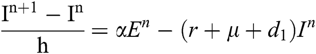
  is the death rate of quarantined people due to COVID-19. The governing equations of the model are as follows:


The above state variables exhibit the nonnegative solution for  with nonnegative initial conditions.
Lemma 1: For any given nonnegative initial conditions, there exist unique solutions  for all
  . Moreover, it satisfies the following inequality of boundedness:
  .
.
Proof: The dynamics of Eqs. (1) to (5) are obtained by adding the five equations, resulting in the following change in the total population:

Thus solutions exist for given initial conditions that are eventually bounded on every finite time interval.
Lemma 2: The closed set  is positively invariant.
Proof: From Eqs. (6) and (7), it follows that as t→∞, the population is bounded by a positive number,
 .
.
Therefore, the set  is positive invariant.
2.2 Steady States of COVID-19 Pandemic Model
There are three steady states of Eqs. (1) to (5), as follows: Trivial equilibrium (TE) = (0,0,0,0,0), corona-free equilibrium (
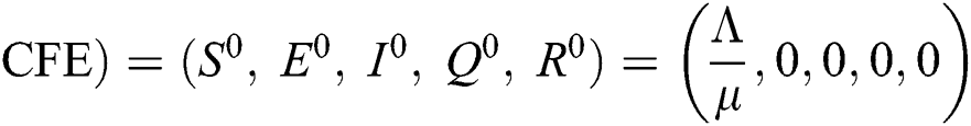 , and corona-present equilibrium (
 ,
,
where  ,
,
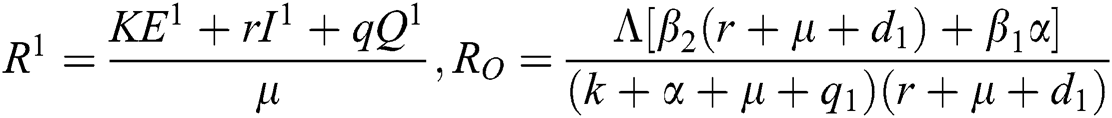 .
.
Note that  is the COVID-19 reproduction number [14].
3 Stochastic COVID-19 Pandemic Model
Let us consider the vector  and the possible changes in the COVID-19 pandemic model, as shown in Tab. 1.
Table 1: Transition probabilities
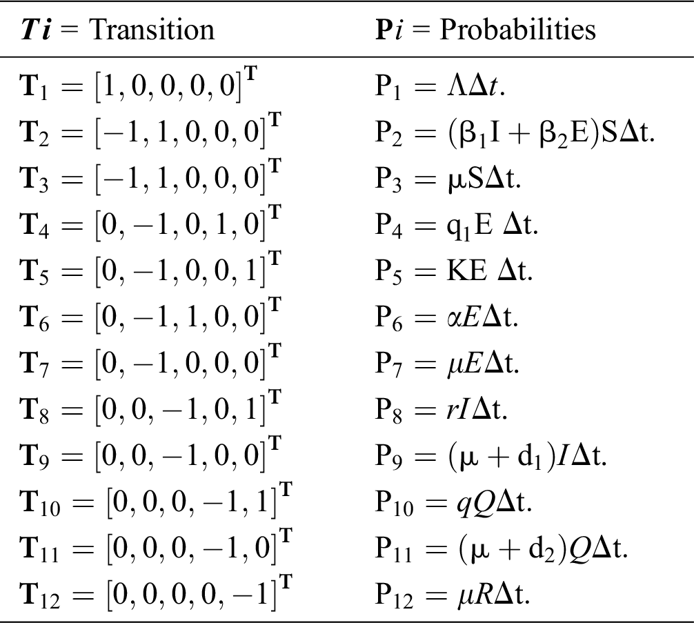
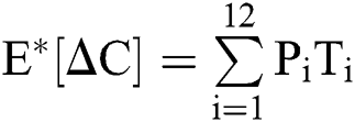
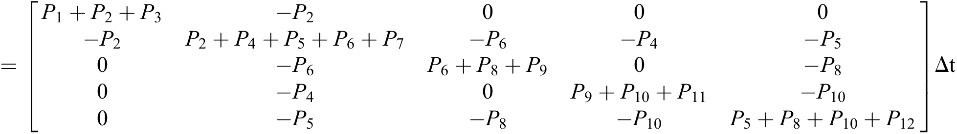
The expectation and variance of the stochastic COVID-19 pandemic model are defined as
 .
.
Expectation 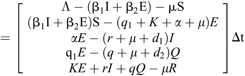
Var = 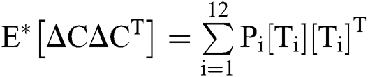
The general form of SDEs is
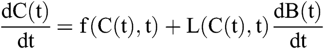
Stochastic drift 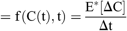
Stochastic diffusion =
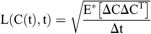 .
.

with initial conditions  , and Brownian motion
  .
.
Raza et al. [14] presented this idea, which can be applied to Eq. (8) as follows:

where  and
and 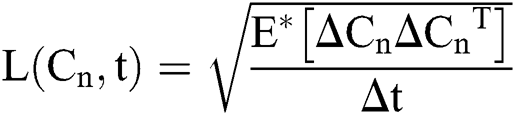 are considered in more detail in Section 3. Also,
  is the time-step size, and
  is normally distributed between stochastic drift and stochastic diffusion, i.e.,
  ).
).
4 Parametric Perturbation in COVID-19 Pandemic Model
Allen et al. [15] presented the following technique. We choose parameters from Eqs. (1) to (5) and change them to random parameters with small noise,  ,
,  . So, the stochastic COVID-19 pandemic model of Eqs. (1) to (5) becomes


The Brownian motion is denoted by  and
and  are the perturbations of Eqs. (10) to (14), which are non-integrable because of Brownian motion. We will use numerical methods to find their solution.
This method can be applied to Eqs. (10) to (14), as follows:


where the time step is  and
and  .s
.s
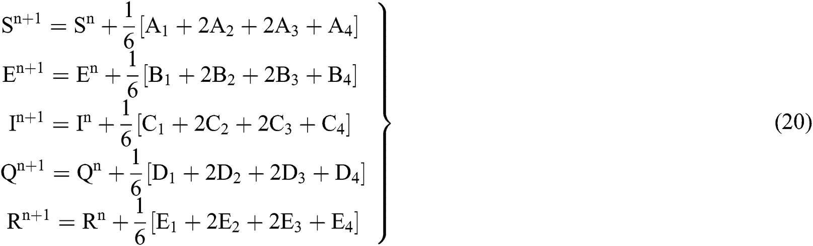
4.2 Stochastic Runge-Kutta Method
This method can be applied to Eqs. (10) to (14), as follows:
Stage 1:


Stage 2:

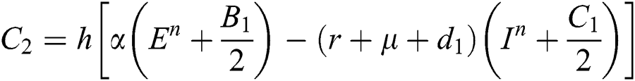
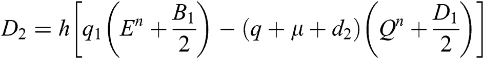

Stage 3:
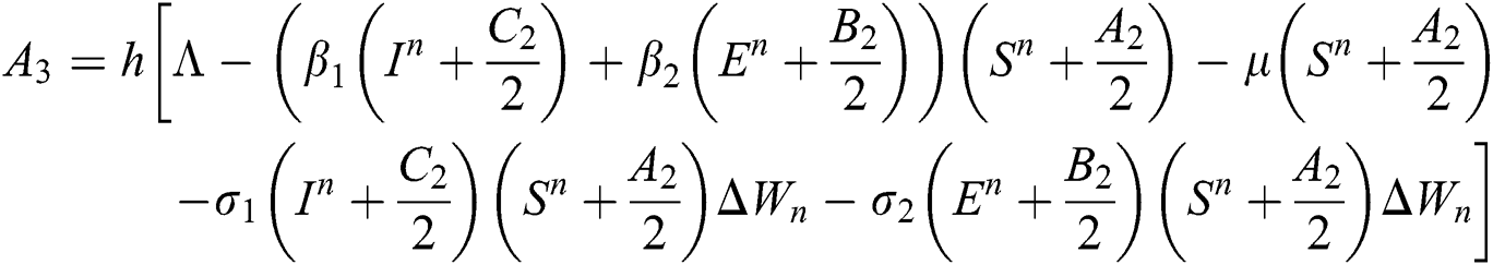
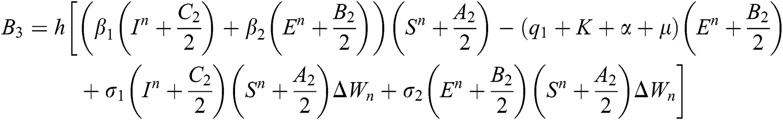
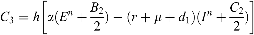
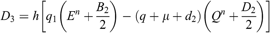

Stage 4:

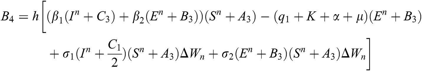


Final stage:
where the time step is  and
and  .
.
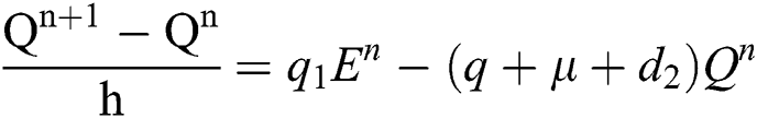
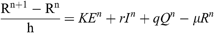
4.3 Stochastic Non-standard Finite Difference Method
This method can be applied to Eqs. (10) to (14), as follows:


where the time step is  and
and  .
.
For essential properties, we shall satisfy the following theorems for positivity, boundedness, consistency, and stability.
Theorem 1: For any given initial value ( (0),
(0), (0),
(0), (0),
(0),  (0),
(0), (0)) ∈
  , Eq. (21) to Eq. (25) have a unique positive solution (
 ∈;
∈;  on n ≥ 0, almost surely.
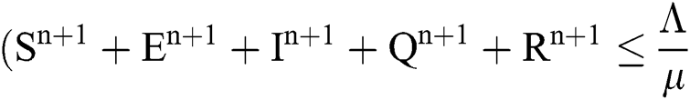
Theorem 2: The region  , for all
  , is a positive invariant feasible region for Eq. (21) to Eq. (25).
Proof: We rewrite Eqs. (21) to (25) as


 .
.
Theorem 3: For any  the discrete dynamical Eqs. (21) to (25) have the same equilibrium as the continuous dynamical Eqs. (10) to (14).
Proof: To solve Eqs. (21) to (25) by assuming the perturbation is zero in the discrete model, we obtain the following three states:
Trivial equilibrium: (T.E) =  (0,0,0,0,0)
Corona-free equilibrium ( :
:
Corona-present equilibrium ( :
:
 ,
,
where
 and
and 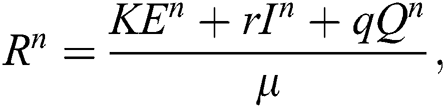
almost surely.
Theorem 4: For any 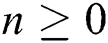 , the proposed numerical method is stable if the eigenvalues of Eqs. (21) to (25) lie in the unit circle [16,17].
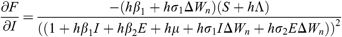
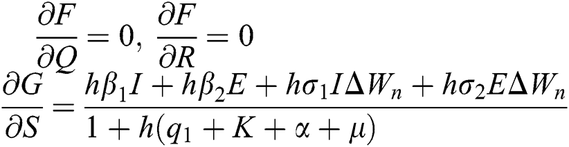
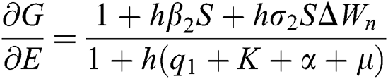
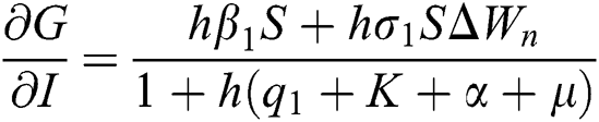
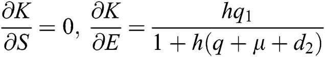
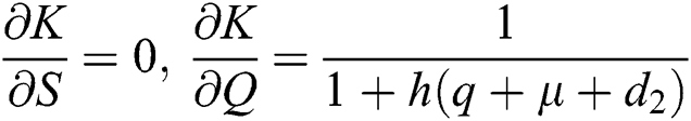
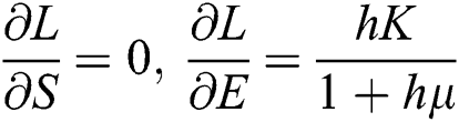
Proof: We consider F, G, H, K, and L from Eqs. (21) to (25), as follows:
 ,
, 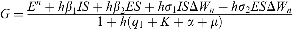 ,
,  ,
,
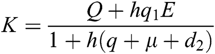 ,
, 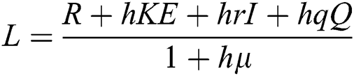 .
.
The Jacobian matrix is defined as
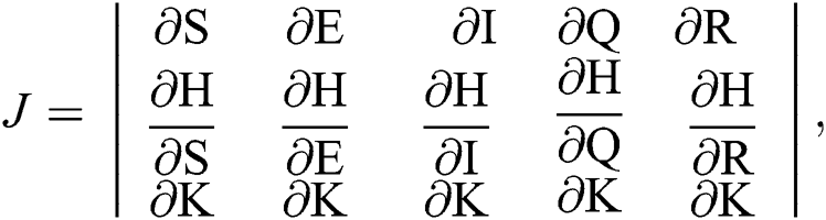 where
where 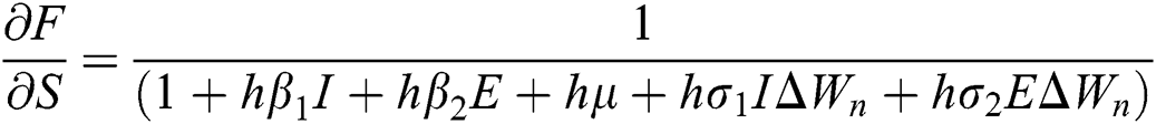

 ,
, 
 ,
, 
 ,
,  ,
, 
 ,
,  ,
, 
 ,
,  ,
,  .
.
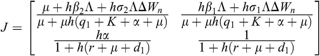
Now, we want to linearize the model about the steady-state of the model for corona-free equilibrium  and
and  .
.
The given Jacobian is
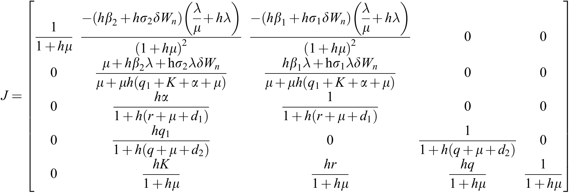
The eigenvalues of the Jacobian matrix are
 ,
, 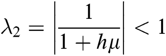 ,
, 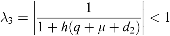 ,
,

 .
.
Lemma 3: For the quadratic equation 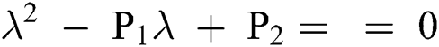 ,
,  , if and only if the following conditions are satisfied:
(i). 
(ii). 
(iii). 
Proof:

 To prove
  ,
,


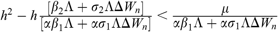


are always satisfied if  .
.

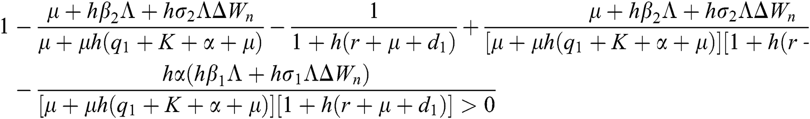


are always satisfied if  .
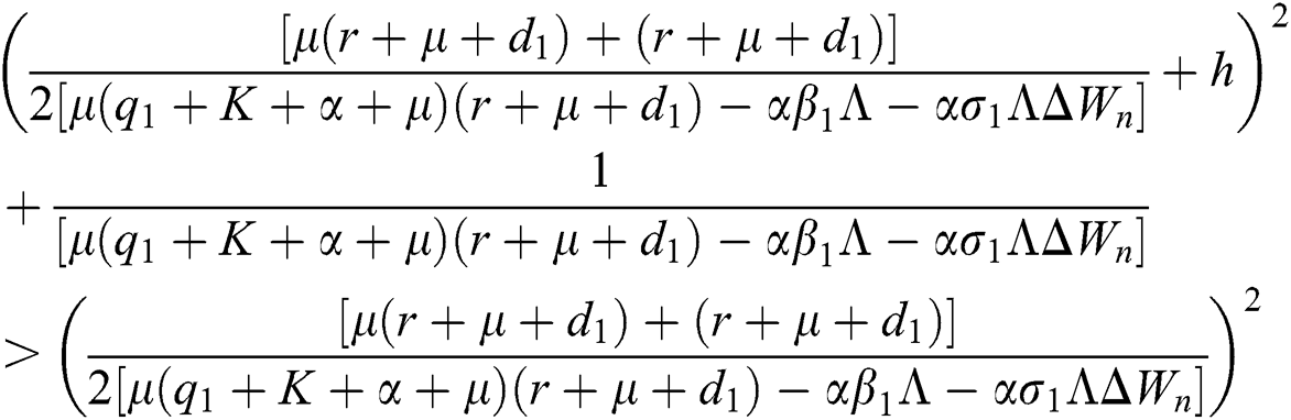
.


 is always satisfied.
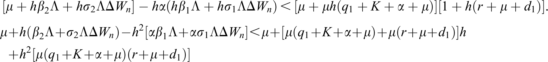
This guarantees that all eigenvalues of the Jacobian lie in the unit circle. So, Eqs. (21) to (25) are stable around  .
.
For the present corona equilibrium, we plot the largest eigenvalue by using fitted values of parameters and MATLAB, as presented in Fig. 1.
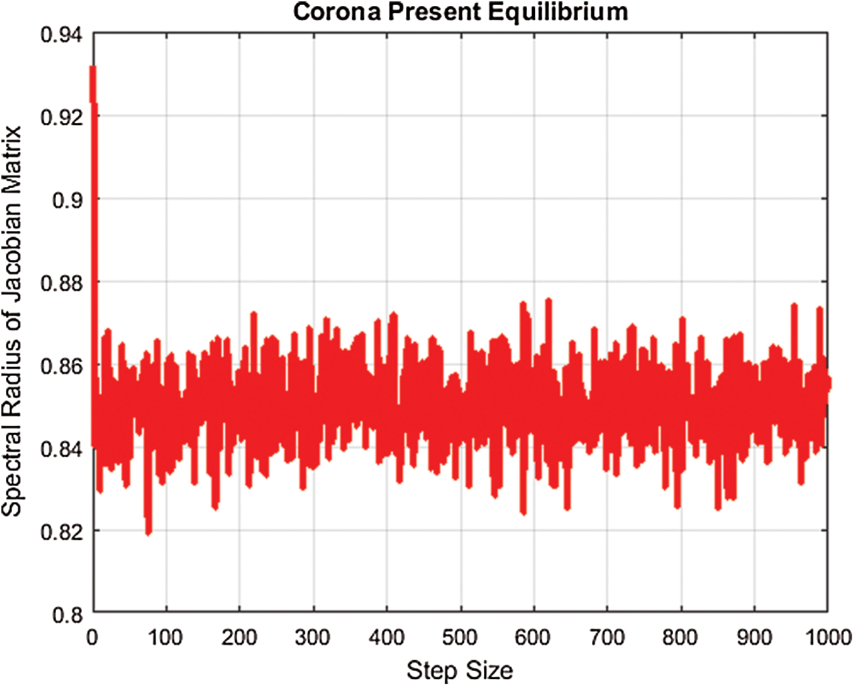
Figure 1: Spectral radius for corona-present equilibrium
Hence, the largest eigenvalue for corona-present equilibrium is less than one. The remaining eigenvalues will be less than one.
The numerical solution is in good agreement with the dynamical behavior of the model using different values of the parameters. Khan et al. [18] assumed the following parameter values:
 ,
,  ,
,  ,
,  ,
,  ,
, ,
,  ,
,  ,
,  ,
,  ,
,  ,
,  ,
,  , for
, for  . For
. For  ,
,  ,
,  ,
,  ,
,  ,
,  ,
, ,
,  ,
,  ,
,  ,
,  ,
,  ,
,  ,
,  , using different nonnegative initial conditions,
  ,
, ,
,  ,
,  ,
,  . We plot each compartment of the model for corona-free equilibrium in Fig. 2.
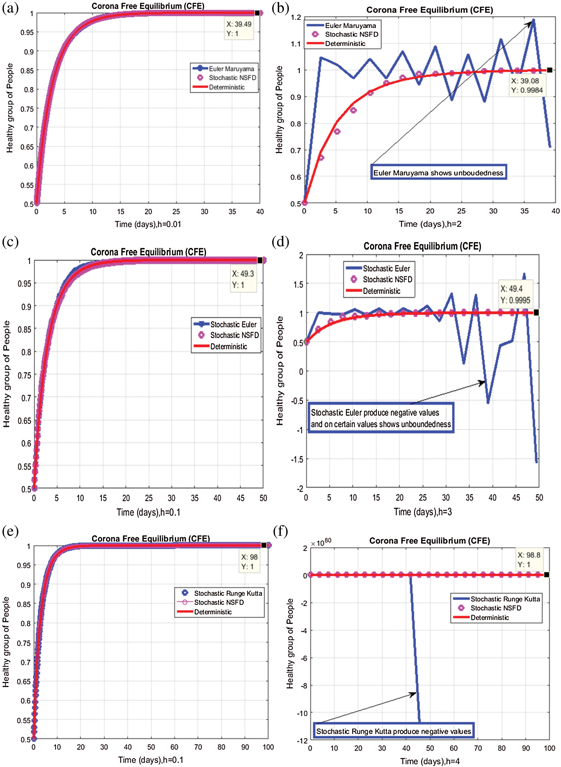
Figure 2: Time plots for different parameters as  ,
,  ,
,  ,
,  ,
, ,
, ,
,  ,
,  ,
,  ,
,  ,
,  ,
,  ,
,  , using initial conditions and
We plot each compartment of the model for corona-present equilibrium in Fig. 3.
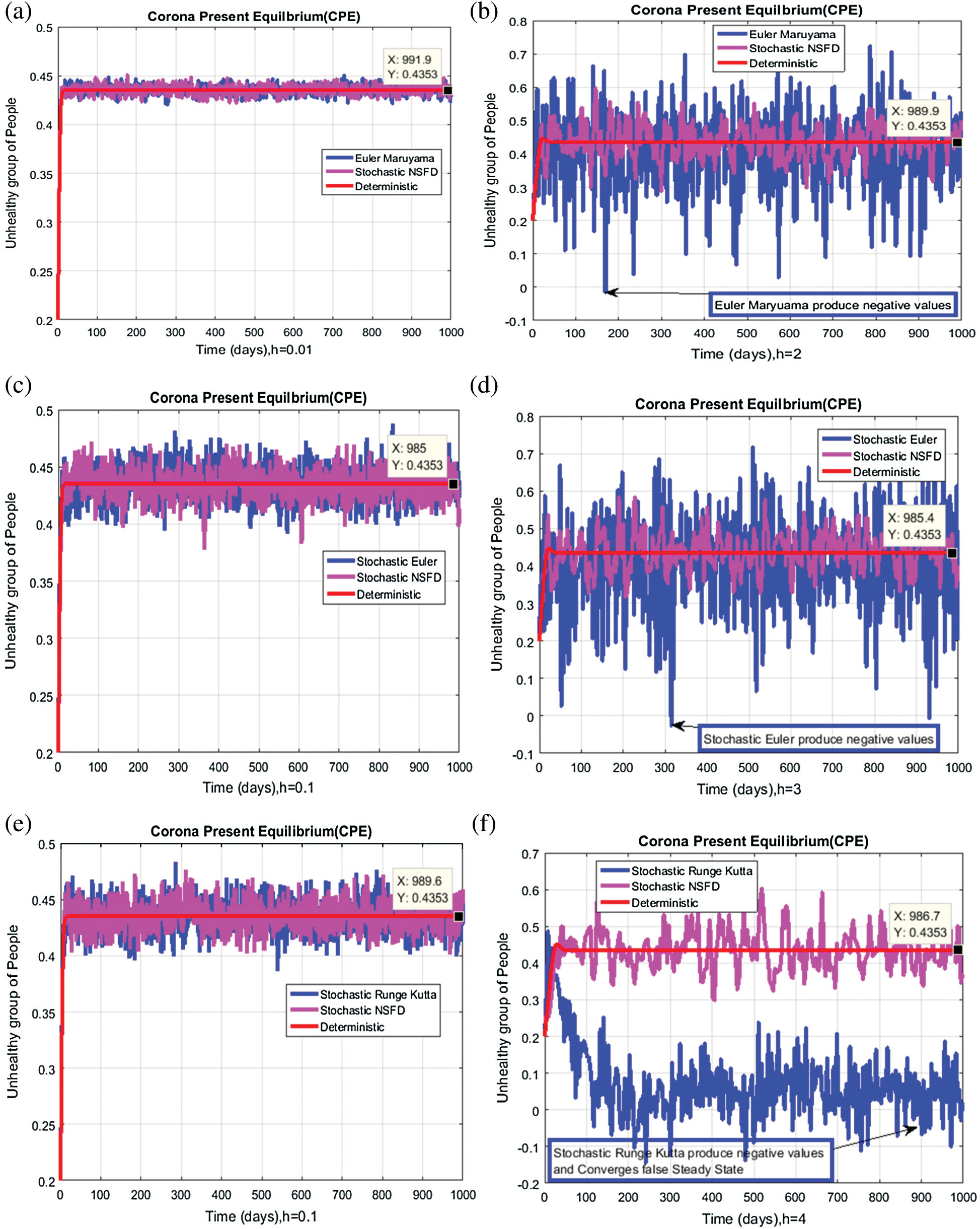
Figure 3: Time plots for different parameters as  ,
,  ,
,  ,
,  ,
, ,
, ,
,  ,
,  ,
,  ,
,  ,
,  ,
,  ,
,  , using the initial conditions and
We plot the solution of Eq. (7) for specific time step sizes in Figs. 2a and 2b. We observe in Fig. 2a that the Euler-Maruyama method converges to corona-free equilibrium. However, in Fig. 2b, the method fails to converge to the true equilibrium of the model. This can be observed in Fig. 3a and Fig. 3b for corona-present equilibrium. The proposed method still converges to the true equilibrium of the model. We plot the solution of Eqs. (13) to (17) for specific time-step sizes in Figs. 2c and 2d. We observe in Fig. 2c that the stochastic Euler method converges to corona-free equilibrium. But in Fig. 2d, the method fails to converge to the true equilibrium of the model. This can be observed in Figs. 3c and 3d for corona-present equilibrium. We plot the solution of Eq. (18) for specific time-step sizes in Figs. 2e and 2f. We observe that in Fig. 2e, the stochastic Runge–Kutta method converges to corona-free equilibrium. But in Fig. 2f, the stochastic Runge–Kutta method fails to converge to the true equilibrium of the model. This can be observed in Figs. 3e and 3f for corona-present equilibrium. So, current numerical methods are time-dependent and violate the essential properties of the model. Thus the proposed method is reliable for finding the solution of epidemiological models, and it always preserves the essential properties of the model.
6 Conclusion and Future Directions
In comparison to the model’s, we have to say stochastic analysis of the most practical and actual model. The explicit numerical methods are conditionally convergent and depend on the time-step size. The stochastic NSFD method is independent of the time-step size. This method is unconditionally convergent as compared to other explicit numerical methods. This method preserves all essential properties of stochastic models, such as consistency, stability, positivity, and boundedness [19]. We will extend our research in all fields of stochastic calculus in the future, and we will extend this concept to stochastic spatiotemporal and stochastic artificial intelligence models [20].
Acknowledgement: We always warmly, thanks to anonymous referees. We are also grateful to Vice-Chancellor, Air University, Islamabad, for providing an excellent research environment and facilities. The first and fourth author also thanks Prince Sultan University for funding this work through the COVID-19 Emergency Research Program.
Funding Statement: This research project is funded by the Research and initiative center COVID-19-DES-2020-65, Prince Sultan University.
Conflicts of Interest: The authors declare that they have no conflicts of interest to report regarding the present study.
1. T. M. Chen, J. Rui, Q. P. Wang, Z. Y. Zhao, J. A. Cui . (2020). et al., “A mathematical model for simulation the phase-based transmissibility of a novel coronavirus,” Infectious Diseases Poverty, vol. 9, no. 24, pp. 1–8. [Google Scholar]
2. T. M. Li, H. C. Chao and J. Zhang. (2019). “Emotion classification based on brain wave: A survey,” Human Centric Computing and Information Sciences, vol. 42, no. 9, pp. 1–17. [Google Scholar]
3. A. J. Kucharski, T. W. Russell, C. Diamond, Y. Liu and J. Edmunds. (2020). “Early dynamics of transmission and control of COVID-19: A mathematical modelling study,” Lancet Infectious Diseases, vol. 11, no. 2, pp. 1–17. [Google Scholar]
4. Q. Lin, S. Zhao, D. Gao, Y. Lou, S. Yang . (2020). et al., “A conceptual model for the coronavirus disease 2019 (COVID-19) outbreak in Wuhan, China with individual reaction and government action,” International Journal of Infectious Diseases, vol. 93, no. 1, pp. 211–216. [Google Scholar]
5. M. D. Shereen, S. Khan, A. Kazmi, N. Bashir and R. Siddique. (2020). “COVID-19 infection: Origin, transmission and characteristics of human coronaviruses,” Journal of Advanced Research, vol. 24, no. 2, pp. 91–98. [Google Scholar]
6. S. Zhao and H. Chen. (2020). “Modeling the epidemic dynamics and control of COVID-19 outbreak in China,” Quantitate Biology, vol. 11, no. 1, pp. 1–9. [Google Scholar]
7. M. Tahir, S. I. A. Shah, G. Zaman and T. Khan. (2019). “Stability behavior of mathematical model MERS corona virus spread in population,” Filomat, vol. 33, no. 12, pp. 3947–3960. [Google Scholar]
8. E. Shim, A. Tariq, W. Choi and G. Chowell. (2020). “Transmission potential and severity of COVID-19 in South Korea,” International Journal of Infectious Diseases, vol. 17, no. 2, pp. 1–19. [Google Scholar]
9. A. Raza, D. Baleanu, M. Rafiq, M. S. Arif, M. Naveed . (2019). et al., “Competitive numerical analysis for stochastic HIV/AIDS epidemic model in a two-sex population,” IET Systems Biology, vol. 13, no. 6, pp. 305–315. [Google Scholar]
10. K. Abodayeh, A. Raza, M. S. Arif, M. Rafiq, M. Bibi . (2020). et al., “Stochastic numerical analysis for impact of heavy alcohol consumption on transmission dynamics of Gonorrhoea epidemic,” Computers Materials & Continua, vol. 62, no. 3, pp. 1125–1142. [Google Scholar]
11. S. Deivalakshmi, P. Palanisamy and X. Z. Gao. (2019). “Balanced GHM mutiwavelet transform based contrast enhancement technique for dark images using dynamic stochastic resonance,” Intelligent Automation and Soft Computing, vol. 25, no. 3, pp. 459–471. [Google Scholar]
12. S. X. Wang, J. He and C. Wang. (2018). “The definition and numerical method of final value problem and arbitrary value problem,” Computer Systems Science and Engineering, vol. 33, no. 5, pp. 379–387. [Google Scholar]
13. O. Driekmann, J. A. P. Heesterbeek and M. G. Roberts. (2009). “The construction of next-generation matrices for compartmental epidemic models,” Journal of Royal Society and Interface, vol. 7, no. 47, pp. 873–885.
14. A. Raza, M. S. Arif and M. Rafiq. (2019). “A reliable numerical analysis for stochastic gonorrhea epidemic model with treatment effect,” International Journal of Biomathematics, vol. 12, no. 5, pp. 445–465. [Google Scholar]
15. E. J. Allen, L. J. S. Allen, A. Arciniega and P. E. Greenwood. (2008). “Construction of equivalent stochastic differential equation models,” Stochastic Analysis and Applications, vol. 26, no. 2, pp. 274–297. [Google Scholar]
16. H. Jansen and E. H. Twizell. (2002). “An unconditionally convergent discretization of the SEIR model,” Mathematics and Computer Simulation, vol. 58, no. 1, pp. 147–158. [Google Scholar]
17. A. J. Arenas, G. G. Parra and B. M. C. Charpentier. (2010). “A non-standard numerical scheme of predictor-corrector type for epidemic models,” Computers and Mathematics with Applications, vol. 59, no. 1, pp. 3740–3749. [Google Scholar]
18. M. A. Khan and A. Atangana. (2020). “Modeling the dynamics of novel coronavirus (219-nCov) with fractional derivative,” Alexandria Engineering Journal, vol. 2, no. 33, pp. 1–11. [Google Scholar]
19. R. E. Mickens. (2005). “A fundamental principle for constructing non-standard finite difference schemes for differential equations,” Journal of Difference Equations and Applications, vol. 11, no. 2, pp. 645–653. [Google Scholar]
20. G. T. Tilahun, O. D. Makinde and D. Malonza. (2017). “Modelling and optimal control of typhoid fever disease with cost effective strategies,” Computational and Mathematical Methods in Medicine, vol. 2, no. 32, pp. 1–18. [Google Scholar]
 | This work is licensed under a Creative Commons Attribution 4.0 International License, which permits unrestricted use, distribution, and reproduction in any medium, provided the original work is properly cited. |