DOI:10.32604/cmc.2020.012314
| Computers, Materials & Continua DOI:10.32604/cmc.2020.012314 | |
| Article |
Analysis and Dynamics of Fractional Order Mathematical Model of COVID-19 in Nigeria Using Atangana-Baleanu Operator
1Department of Mathematics, University of Ilorin, Ilorin, Kwara, Nigeria
2Department of Mathematics, AKI’s Poona College of Arts, Science and Commerce, Camp, Pune, India
3Department of Mathematics, College of Arts and Sciences, Prince Sattam bin Abdulaziz University, Wadi Aldawaser, Saudi Arabia
4Department of Mathematics, Cankaya University, Ankara, 06790, Turkey
5Institute of Space Sciences, Magurele-Bucharest, 077125, Romania
6Department of Medical Research, China Medical University Hospital, China Medical University, Taichung, 40447, Taiwan
7Faculty of Mathematics and Statistics, Ton Duc Thang University, Ho Chi Minh City, Vietnam
*Corresponding Author: Amjad S. Shaikh. Email: amjatshaikh@gmail.com
Received: 25 June 2020; Accepted: 30 August 2020
Abstract: We propose a mathematical model of the coronavirus disease 2019 (COVID-19) to investigate the transmission and control mechanism of the disease in the community of Nigeria. Using stability theory of differential equations, the qualitative behavior of model is studied. The pandemic indicator represented by basic reproductive number R0 is obtained from the largest eigenvalue of the next-generation matrix. Local as well as global asymptotic stability conditions for the disease-free and pandemic equilibrium are obtained which determines the conditions to stabilize the exponential spread of the disease. Further, we examined this model by using Atangana–Baleanu fractional derivative operator and existence criteria of solution for the operator is established. We consider the data of reported infection cases from April 1, 2020, till April 30, 2020, and parameterized the model. We have used one of the reliable and efficient method known as iterative Laplace transform to obtain numerical simulations. The impacts of various biological parameters on transmission dynamics of COVID-19 is examined. These results are based on different values of the fractional parameter and serve as a control parameter to identify the significant strategies for the control of the disease. In the end, the obtained results are demonstrated graphically to justify our theoretical findings.
Keywords: Mathematical model; COVID-19; Atangana-Baleanu fractional operator; existence of solutions; stability analysis; numerical simulation
The ongoing ravaging COVID-19 is a contagious disease instigated by SARS-CoV-2. The first case of the disease was reported in December 2019 in Wuhan, China, and has, within few weeks, spread across the globe, leading to the present 2020 COVID-19 pandemic [1]. The coronavirus disease 2019 has been regarded as the largest global health crisis in human history as a result of the magnitude of confirmed cases, accompanied by the degree of fatalities across the continents [2]. Reliable data had it that by April 2020, COVID-19 pandemic had led to over 3 million confirmed cases with 230,000 deaths and the disease has spread to over 210 nations globally [3]. The symptoms and signs of COVID-19 develop within 2 to 14 days [4]. When the disease is fully incubated, the infected individuals may exhibit fever, fatigue, cough and breathing disorder that is similar to those infections instigated by SARS-CoV and MERS-CoV [5]. However, many COVID-19 acute cases and fatalities come from the elderly people (from the age of 65 upward) and individuals with severe health challenges (such as people with kidney disease, hypertension, diabetes, obesity and other health issues that deteriorate the immune system) [3].
The first confirmed case in Nigeria was reported on 27 February 2020, when a citizen from Italy is tested positive for the virus [6]. The disease transmission raised gradually over the month of April 2020, after a substantial number of cases were noted for in the country. Since then, Nigeria is focused on spotting and referring identified infectious patients for treatment to devoted COVID-19 centers. As of 18 June 2020, Nigeria had reported 17,735 confirmed cases out of which 11,299 are active cases, 5,967 recovered peoples and 469 deaths due to COVID-19 infection [7].
The global scourge of COVID-19 pandemic has elicited the attention of scholars in different disciplines, prompting several proposals to examine and envisage the development of the pandemic [8]. Ndairov et al. [9] propose a model for the transmissibility of COVID-19 in the presence of super-spreaders individuals. They perform the stability and sensitivity analyses of the model and discovered that daily reduction in the number of confirmed cases of COVID-19 is a function of the number of hospitalizations. Yang et al. [10] proposed a model to study the transmission pathways of COVID-19 in terms of human-to-human and environment-to-human spread. Their analysis confirms the tendency of COVID-19 to remain pandemic even with prevention and intervention measures.
A model for the dynamics of COVID-19 with parameter estimations, sensitivity analysis and data fitting is investigated in [11] while a model for COVID-19 infection that describes the impact of slow diagnosis on the dynamics of COVID-19 is also studied in [12]. In [13], the researchers employ a statistical study of coronavirus disease data to calculate time-regulated risk for fatality from the COVID-19 in Wuhan. Their results indicate that movement restrictions and adequate social distancing procedures are capable of reducing the spread of the disease. Furthermore, a data-oriented model that includes behavioral impacts of humans and governmental efforts on the dynamics of COVID-19 in Wuhan is proposed in [14]. A good number of mathematics and non-mathematics studies have also been conducted on COVID-19 [15–21].
In recent times, the integer order differential systems are generalized and improved in order to formulate several mathematical models using fractional differential operators. Since, demonstration of some real-world phenomena with the help of fractional derivative operator is more appropriate and useful for improving performance of numerous engineering and applied sciences systems [22–29]. In this paper, initially we formulate the mathematical model in terms of integer order derivative and then apply the Atangana–Baleanu fractional derivative operator. The motivation behind utilizing the Atangana–Baleanu operator is that it has nonlocal and nonsingular kernel in the form of Mittag-Leffler function. Moreover, the complex behavior in the model must be ideal portrayed utilizing this operator. Literature pertaining to Atangana–Baleanu derivative and their applications to several systems arising in the field of applied sciences and engineering can be cited in [30–34].
The population of human under consideration is divided into six compartments which are susceptible S(t), since the incubation period of COVID-19 is between two to fourteen days there are those who are infected without exhibiting any sign of symptoms and are undetected E(t). Individuals who are infected or suspected case of COVID-19 need to go through an incubation period before the suspected symptom can noticeable these categories are quarantined Q(t), there are those certain proportion of the population have been infected with sign and symptoms of COVID-19 and is highly infectious but not yet quarantined or isolated I(t). C(t) represent confirmed case of COVID-19 from Quarantine category. R(t) represent recovery after treatment. The susceptible population is increased by immigration or by birth at the rate  , in each of the class, individuals can die a natural death and the rate
  , there is a force of infection between the susceptible population and exposed population this is represented by
  ,
,  represent the progression from exposed class to highly infected class, the disease induced death rate for highly infected class, quarantine class and confirmed case of COVID-19 class is represented by
  , proportion of people identified as suspected case of COVID-19 are represented by
  , after medical diagnosis, some of the suspected cases were confirmed, others that are not detected can return back to the susceptible population at the rate
  . In the meantime, some highly infectious individuals will be moved to quarantine class at the rate
  . The progression rate from quarantine to confirm case after diagnosis is denoted by
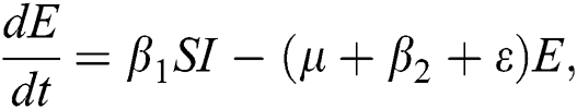
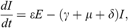
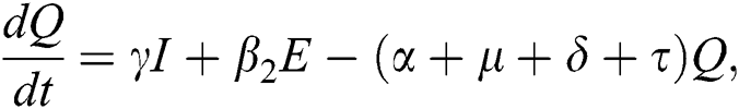
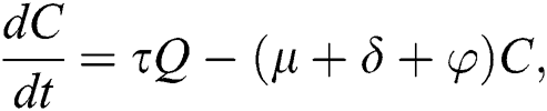
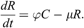
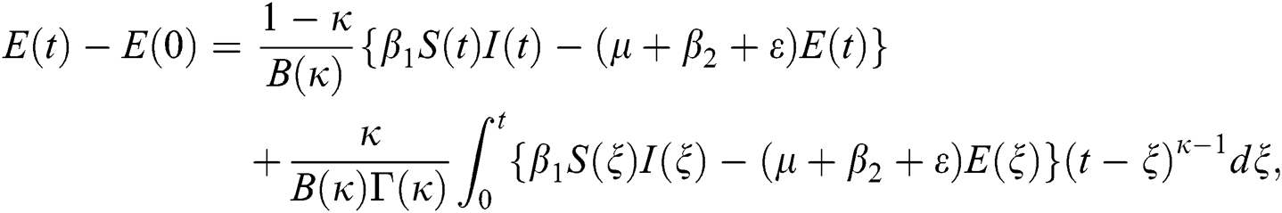
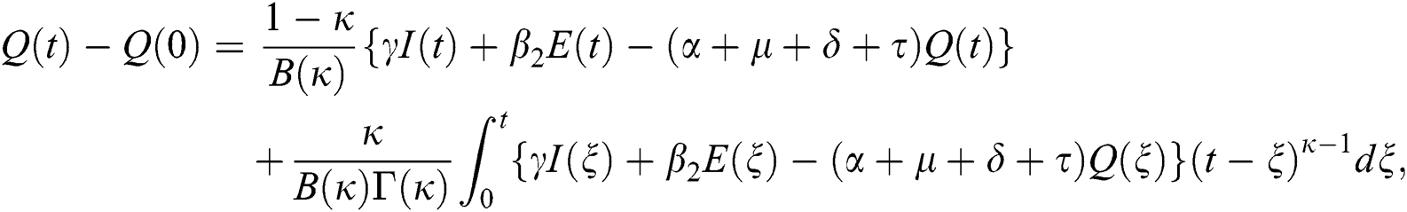
  . The pictorial diagram illustrating the model is shown in Fig. 1 while the system of equations governing the model is given as:
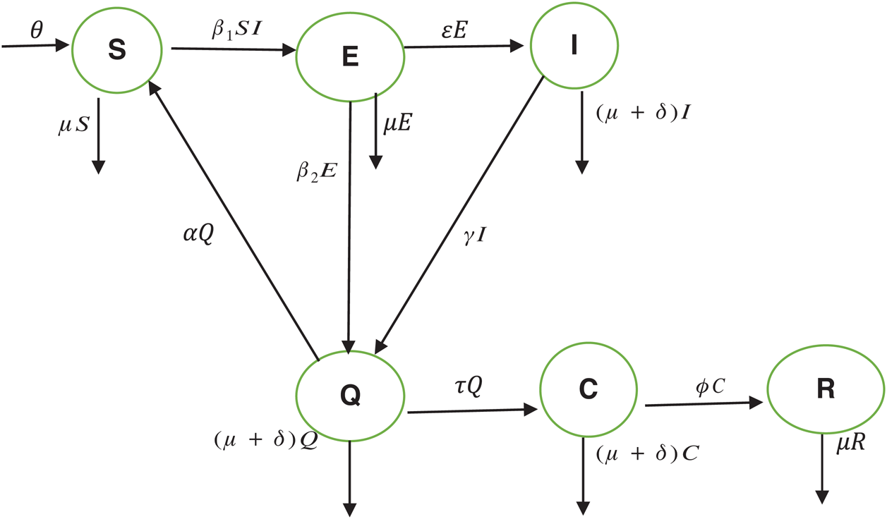
Figure 1: The model’s flow diagram

The rest of the sections are organized as follows: Some valuable preliminaries dependent on the Atangana–Baleanu fractional operator is given in Section 3. In Section 4, we present stability analysis of the equilibria (drug-free equilibrium state and endemic equilibrium state). Analysis of fractional coronavirus model using the Atangana–Baleanu operator is given in Section 5. The Approximation technique and Numerical Simulation are given to reveal the behavior of dynamics components is accounted for in Section 6. The conclusion is finally drawn in the last Section 7.
This section of the paper will convert some basic definitions and properties related to Fractional calculus. During the paper process, we are going to refer to the following given specific definitions and properties of the Atangana–Baleanu fractional derivatives of Caputo type [32] that are peculiar to our study.
Definition 3.1 The Caputo fractional derivative for order  is defined as
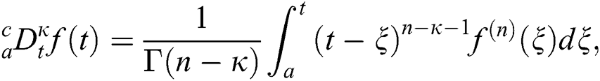
where 
Definition 3.2 The Atangana–Baleanu fractional derivative for a given function for order  in Caputo sense are defined as
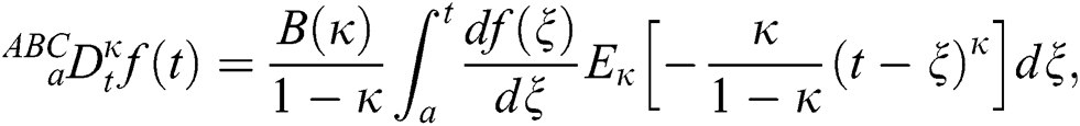
where 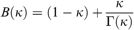 is a normalization function and
  is the Mittag-Leffler function.
Definition 3.3 Atangana–Baleanu fractional integral order  is defined as
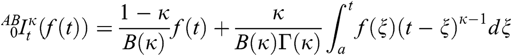
if  is a constant, integral will be resulted with zero.
Definition 3.4 The Laplace transforms for the Atangana–Baleanu fractional operator of order  where 0
  is given as
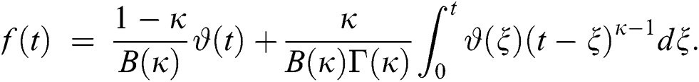
Theorem 3.1. The following time fractional ordinary differential equation
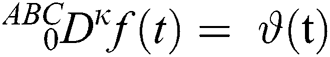
has a unique solution considering the inverse Laplace transform and the convolution property below
4 Basic Properties of the Model
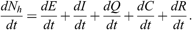
The invariant region sets out the domain where the model’s solutions are both biologically and mathematically meaningful. Since the model deals with human population, all of the model’s variables and parameters are assumed to be positive. To achieve this, we consider first the total human population Nh, where Nh = S + E + I + Q + C + R.
By differentiating with respect to t both side of the total population N

In the absence of the disease induced death due to COVID-19 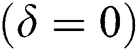 , Eq. (2) becomes
Integrating on both side

with the initial condition  , where A is constant. Applying the initial condition in Eq. (4), we get
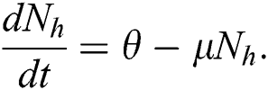
As  in Eq. (5), the total human population reduces to
  . In this regard, all the feasible solution sets for human population in Eq. (1) enters and remains in the region
We therefore conclude that the proposed model is well posed and are both biologically and mathematically meaningful in the domain  .
.
For the COVID-19 model dynamics in Eq. (1) to be epidemiologically meaningful it is important to prove that all its state variables are positive for all time.
Theorem 4.1
Let the  . Then the solutions
  are non-negative for
  .
.
First, we consider the susceptible compartment in Eq. (1) give as 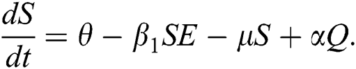

By applying the initial condition  and solving the above Eq. (7), we get
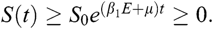
By repeating the same procedure for  respectively in the system Eq. (1), we obtained the following results


This shows that the solutions of the model are positive. Hence the proof.
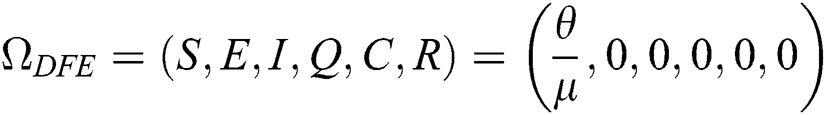
4.3 Disease-Free Equilibrium State (DFE)
The COVID-19 model in Eq. (1) has a disease-free equilibrium DFE obtain by setting the right-hand side of Eq. (1) to zero. Therefore,
4.4 Existence of Endemic Equilibrium Point (EE)
We present the existence of the COVID-19 endemic equilibrium states. It is a positive equilibrium state where the COVID-19 disease is persisting in the population.
Theorem 4.2. Let there be a unique endemic equilibrium state when the basic reproduction number R0 > 1 in the COVID-19 periodically forced model in Eq. (1).
Proof. Suppose  is a nontrivial equilibrium state of system Eq. (1) which then connote that all the compartment of
  are non-negative. By equating the left-hand side of Eq. (1) to zero we get the following endemic equilibrium states
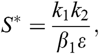
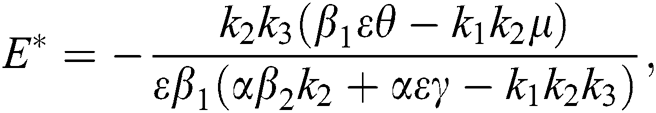
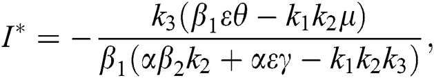
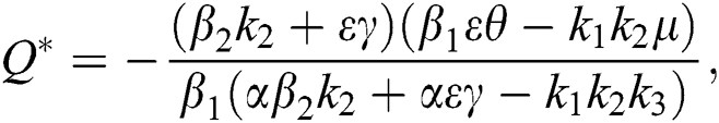
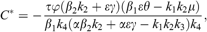
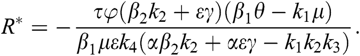
where

4.5 Basic Reproduction Number R0
The basic reproductive ratio is a threshold quantity that represents the overall number of secondary diseases caused by a single infected individual created into a fully susceptible population throughout its infectious period. F and V are the matrices for the new infections generated and the terms of transition. Following the same approach as [35], we have
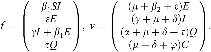
The Jacobian matrix of f and v computed at the disease-free equilibrium is given as F and V such that
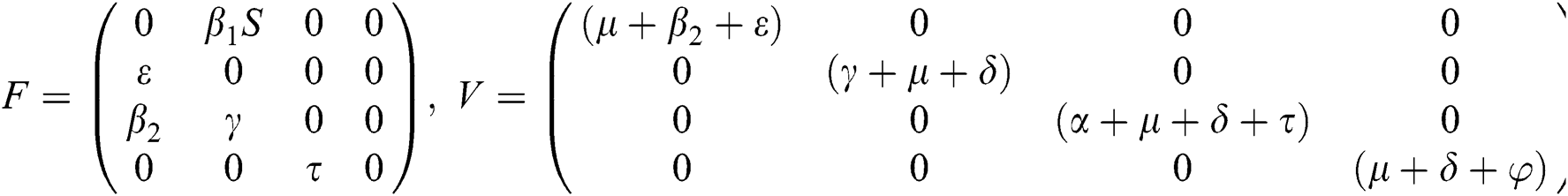
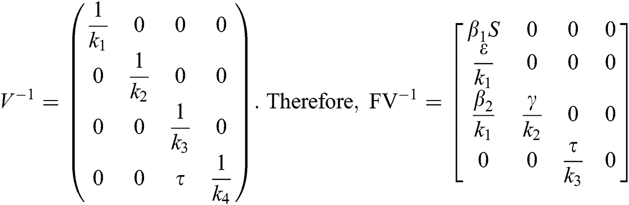
By substituting  and
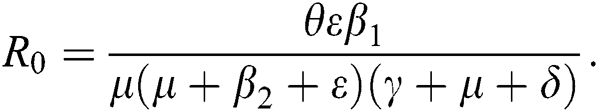
and  from Eq. (11), we therefore obtain the basic reproduction number which is the spectral radius of the matrix
 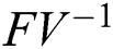 as
as
4.6 Global Stability of the Disease-Free Equilibrium
Theorem 4.3. If  , then the disease-free equilibrium
 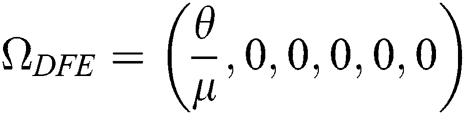 is globally asymptotically stable otherwise it is unstable.
Proof. We consider the Lyapunov function of the type  and
and 
where, 
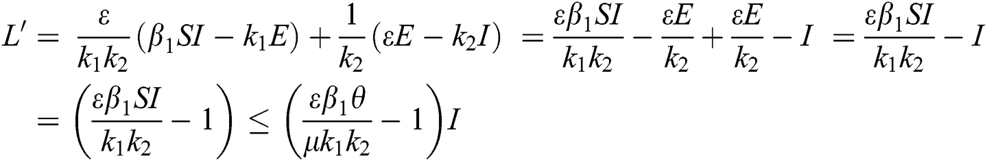
From the result in Eq. (12), we can conclude that  provided that
 . In addition,
  provided that
  or
or  .
.
5 Analysis of Fractional Coronavirus Model Using the Atangana-Baleanu Operator
Let us consider the mathematical model given by an ordinary differential equation system Eq. (1) using Atangana–Baleanu fractional derivative operator as below


where  represents the fractional operator of type Atangana–Baleanu–Caputo (ABC) having fractional order
  where 0
  , subject to initial conditions


The system in Eq. (14) can be converted to the Volterra-type integral equation by using the ABC fractional integral. The model is written by referring Theorem 3.1 as below:


Theorem 5.1 The kernels  and
and  given in Eq. (14) satisfy the Lipschitz condition and contraction if the following inequality holds:

Proof: Let the kernel 
Let  and
and  be two functions; then we obtain the following:


where  .
.
Similarly, we get,


where,
 , and
, and  .
.
Considering the kernels of the model, Eq. (16) can be rewritten as


Therefore, we get the following recursive formula.


We next get the difference between the iterative terms in the expression


where

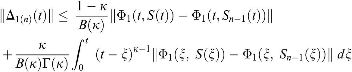
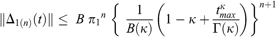
Applying the norm of both sides and considering triangular inequality, the Eq. (21) becomes


Since the kernels satisfy the Lipschitz condition, we get the following


This completes the proof of the theorem.
Theorem 5.2 (Existence of the Solution). The system given by Eq. (14) has a solution under the conditions that we can find  satisfying
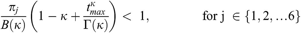 .
.
Proof: Let the functions S(t), E(t), I(t), Q(t), C(t) and R(t) are bounded. From Eq. (23) we get the following relations.
Hence, the functions  and
and  given in Eq. (24) exist and are smooth. Moreover, to show that the functions in Eq. (24) are the solutions of Eq. (14), we assume that


where 
 and
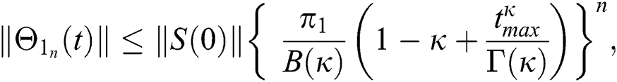
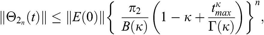
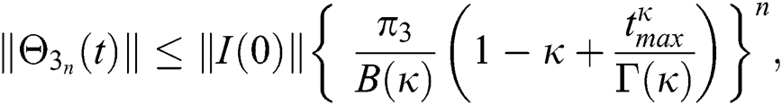
and  are reminder terms of series solution. Then, we must show that these terms approach to zero at infinity, that is,
 ,
, 
and  Thus, for the term
Continuing this way recursively, we get
where 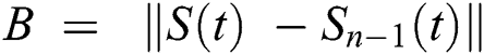 .
.
When we take the limit of both sides as n tends to infinity, we get

6 The Approximation Technique and Numerical Simulation
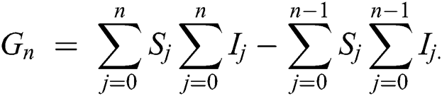
Consider the coronavirus model Eq. (14) along with initial conditions Eq. (15). The terms SI in this model is nonlinear. Implementing the Laplace transform on both sides of Eq. (14), we obtain,
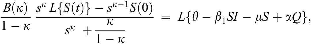
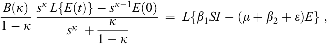
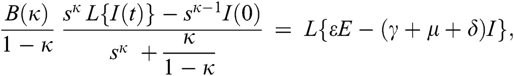
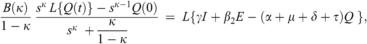
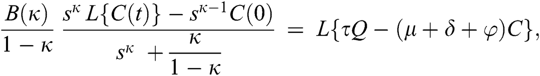

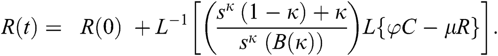
Rearranging, we get
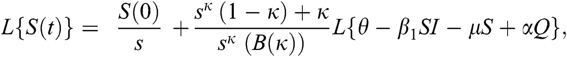

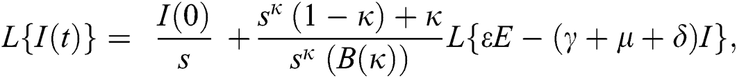

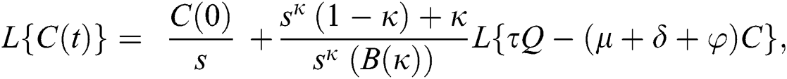
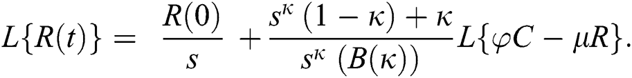
Further, the inverse Laplace transform on Eq. (29), yields


The series solutions achieved by the method are given by,

The nonlinearity of SI is written as 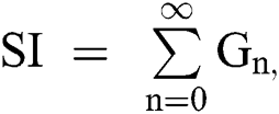 whereas
  is further decomposed as follows [23]
Using initial conditions, we get the recursive formula given by


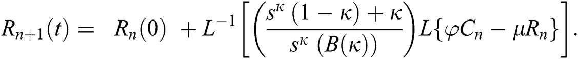
where

The approximate solution is assumed to obtain as a limit when n tends to infinity.


In this section, we have presented data fitting, numerical simulations and graphical demonstration of the Atangana Baleanu COVID-19 model Eq. (14) for the population of Nigeria. We consider the available cumulative infection cases for April 1, 2020, till April 30, 2020 and parameterized the model [36]. The parameters were estimated based on the some assumptions and facts given in Tab. 1 which plays significant role in estimating R0 (basic reproductive number). R0 is expected number of cases directly generated by one individual in a population. When R0 > 1 the infection will be able to start spreading in a population, but if R0 < 1 the disease will die out.
Table 1: Details Defination of Variables and Parameters

Next, we evaluate and present the number of cumulative infectious cases in different compartments with respect to time in days using various plots for population of Nigeria. We begin estimation of our model from initial time (t =  ) as per data reported on April 1, 2020 [6]. Hence, the required initial values are S(0) =
  ; E(0) = 15,000; I(0) = 100; Q(0) = 100; C(0) =175; R(0) = 31.
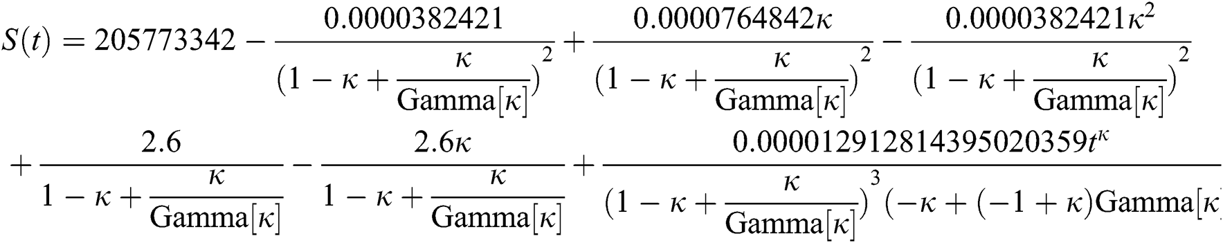
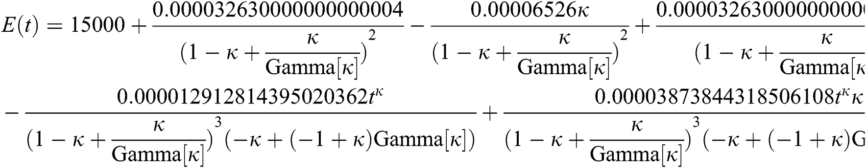
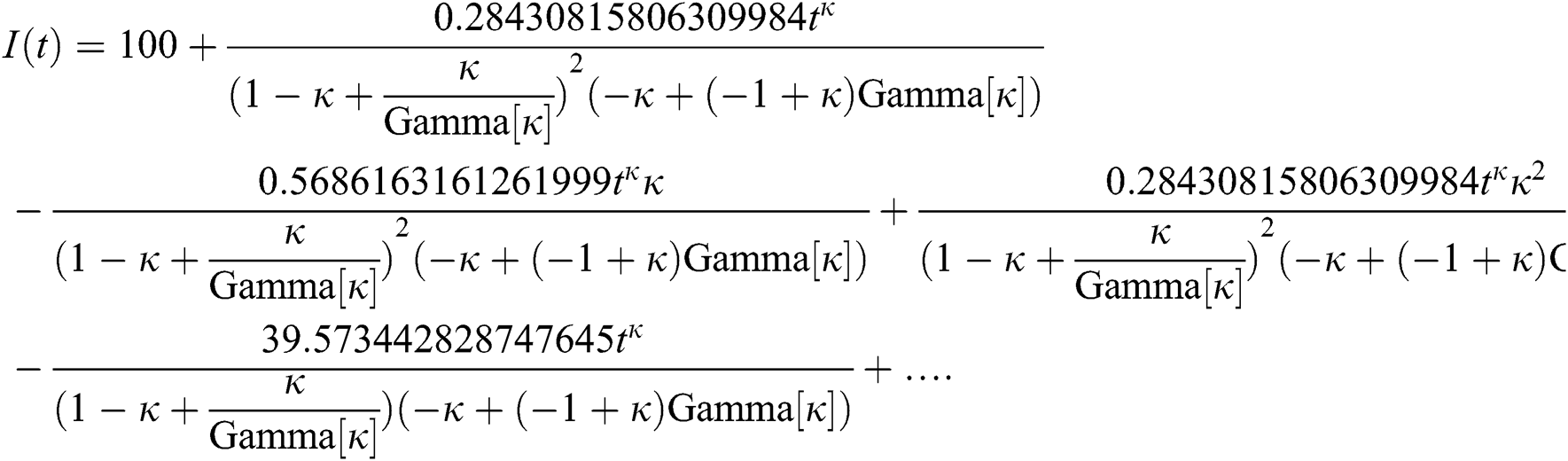
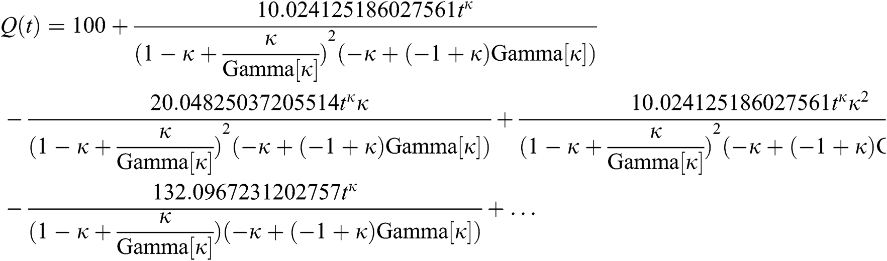
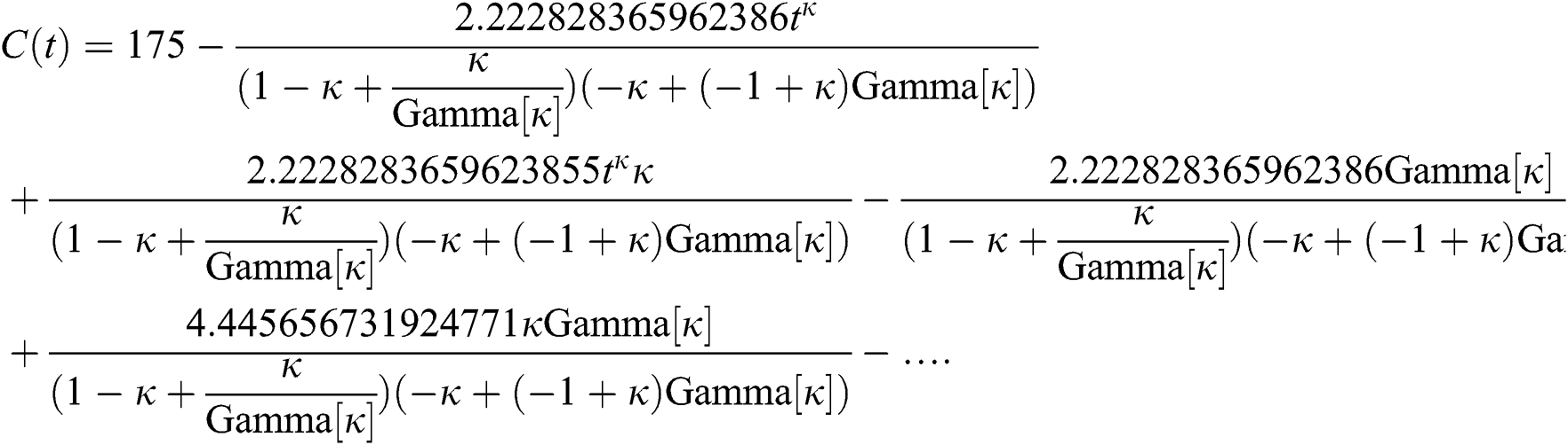
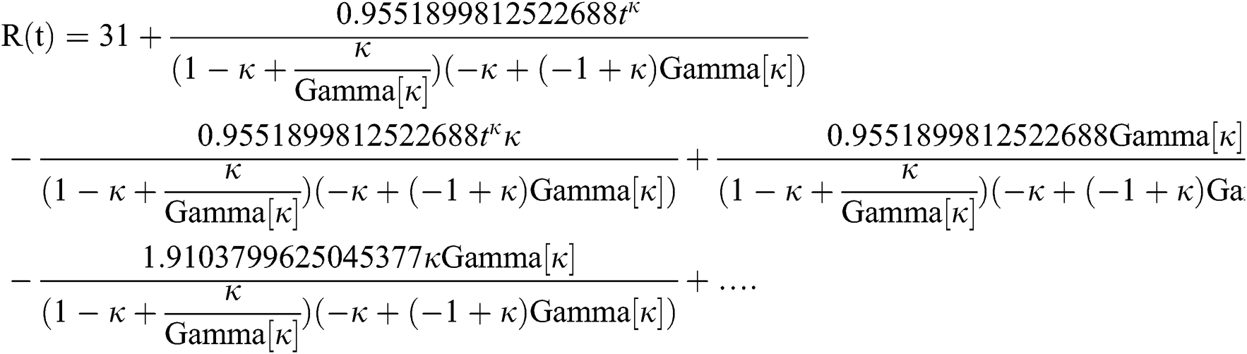
By applying iterative Laplace transform using Eq. (31) successively up to four terms we get series form approximate solution of the fractional COVID-19 model Eq. (14) as given below
In Tab. 1, we have estimated some needed biological parameter values related with basic reproduction number  corresponds to model (1) like, covid-19 infection death rate (
 ), force of infection (
 ), proportion of people identified as suspected cases (
 ), progression rate from exposed class to highly infected class (
 ) and other parameters are fitted from previous literature. Estimating these parameters to suitable values decreases rate of infection meaningfully. It is examined and noted that if
  is near to 2 the number of cumulative infected population rises very quickly. Also reducing the value of
  near to one lowers the number of infected cases rapidly.
Figs. 2a–7b shows the dynamical behaviour of various classes of mathematical model like susceptible population S(t), symptomatic and undetected population E(t), highly infectious but not yet quarantined or isolated I(t), individuals who are infected or suspected and quarantined Q(t), confirmed and quarantine population C(t), recovered population R(t) with  = 1.96 and
  = 1.16 respectively for various values of
  = 1, 0.9, 0.8, 0.7 verses time in days. It is observed that as the value of
  decreases from
  the effect of the fractional derivative order becomes prominent. We clearly observe the significant variance in both type of plots (a) and (b) in each figure when value of fractional parameter
  changes. From Figs. 3a and 3b, it is noticed that as the time increase with respect to time the symptomatic and undetected population E(t) also increases due to spread of infection in the population and their interaction with infected people. It is clear that reducing the value of fractional parameter
  significantly affect COVID-19 dynamics and greatly decrease the fraction of asymptomatic carriers with level of infection in the population. Hence, the number of cumulative cases of infections in every class is continuously depends upon the values of fractional order.
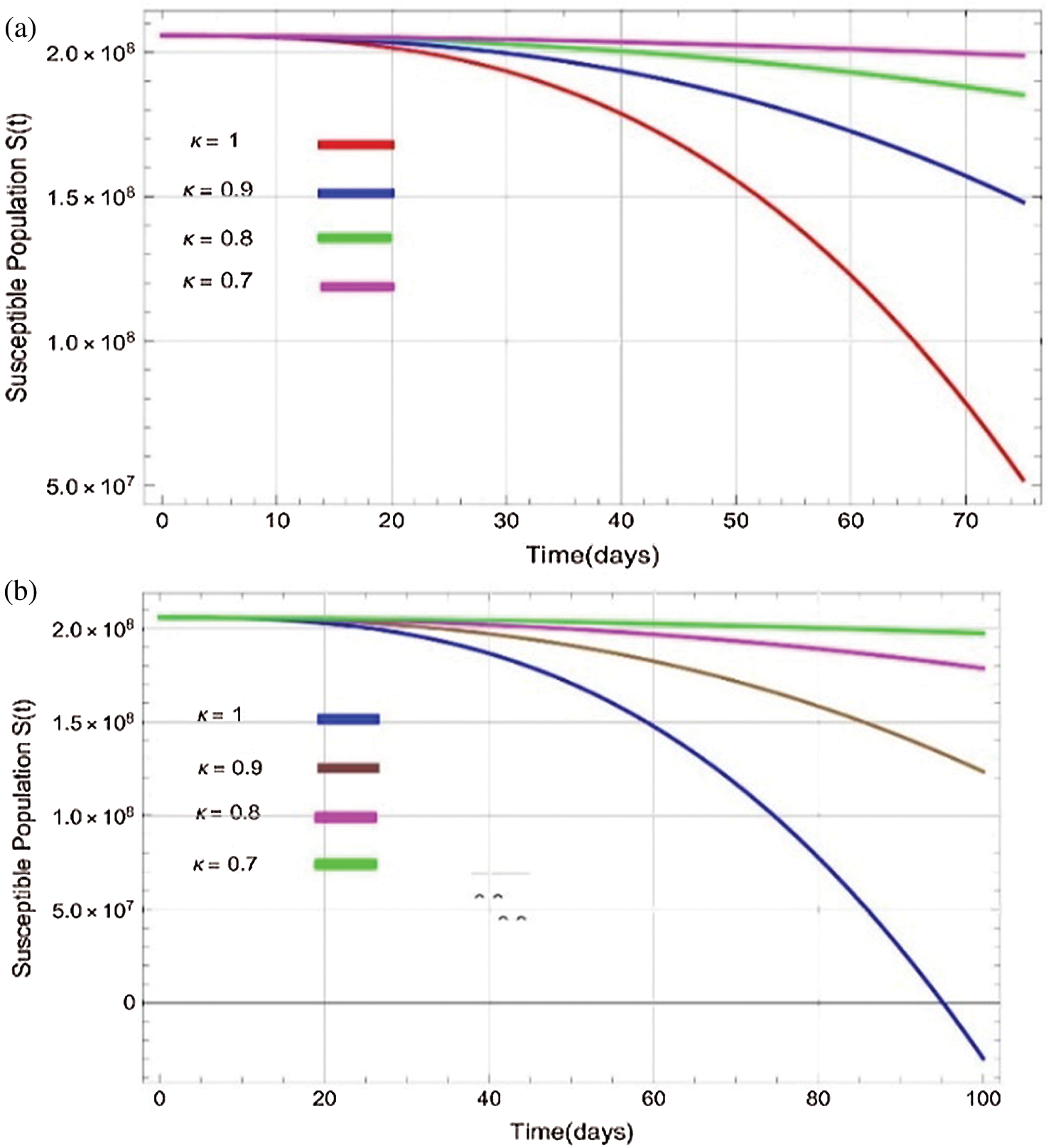
Figure 2: Plots of susceptible population for various values of  with respect to time t in days and different R0 [Fig. 2(a): R0 = 1.96, Fig. 2(b): R0 = 1.16]
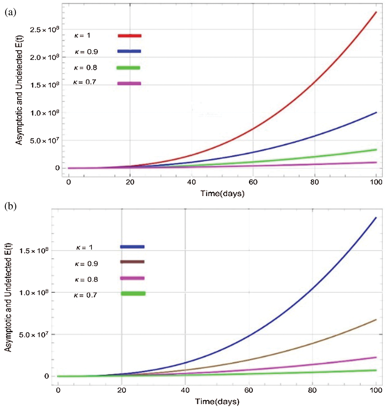
Figure 3: Plots of asymptotic and undected population for various values of  with respect to time t in days and different R0 [Fig. 3(a): R0 = 1.96, Fig. 3(b): R0 = 1.16]
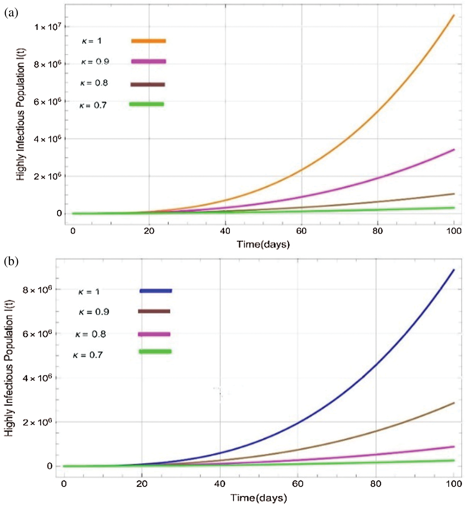
Figure 4: Plots of highly infectitious population for various values of  with respect to time t in days and different R0 [Fig. 4(a): R0 = 1.96, Fig. 4(b): R0 = 1.16]
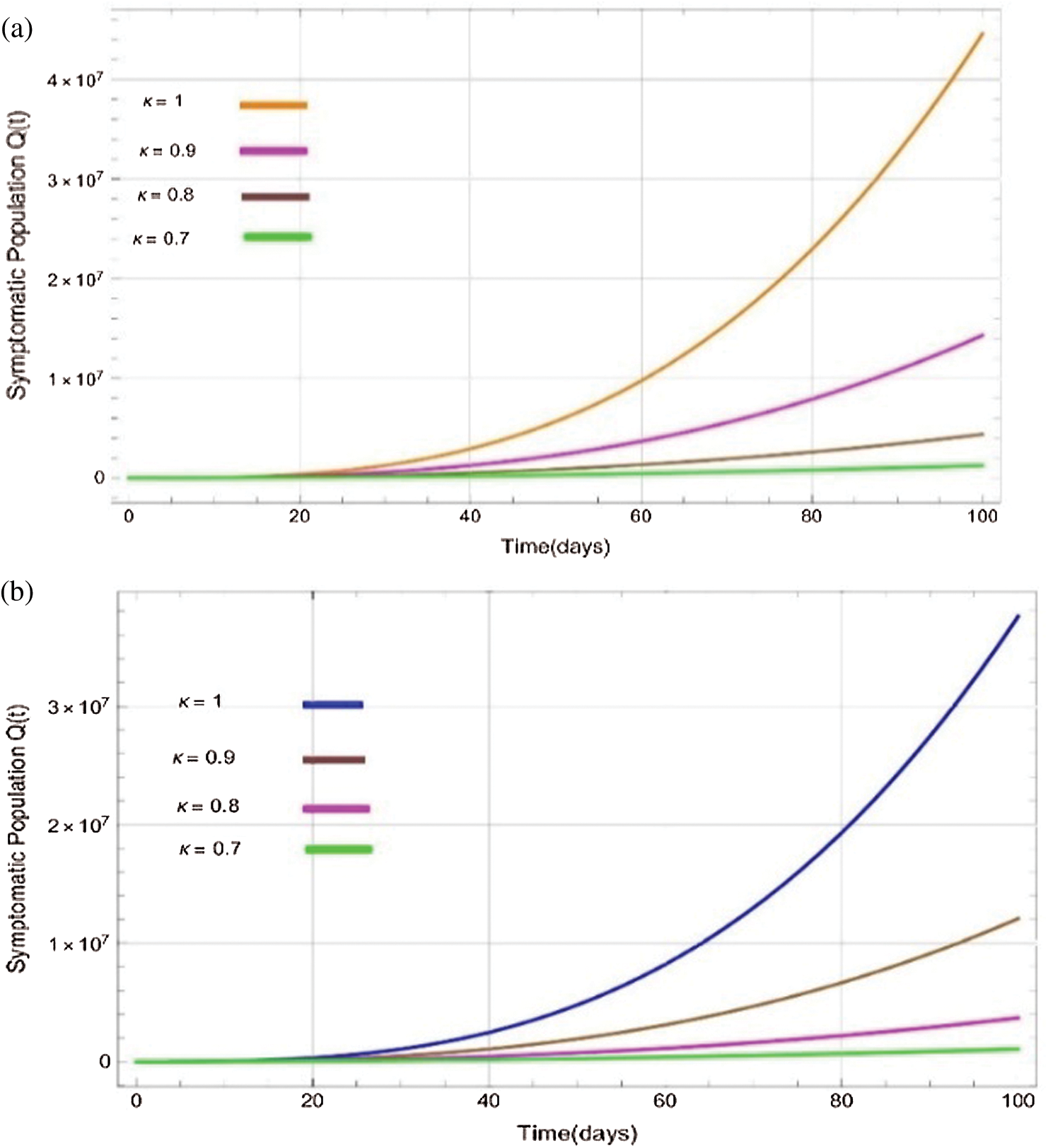
Figure 5: Plots of symptomatics population for various values of  with respect to time t in days and different R0 [Fig. 5(a): R0 = 1.96, Fig. 5(b): R0 = 1.16]
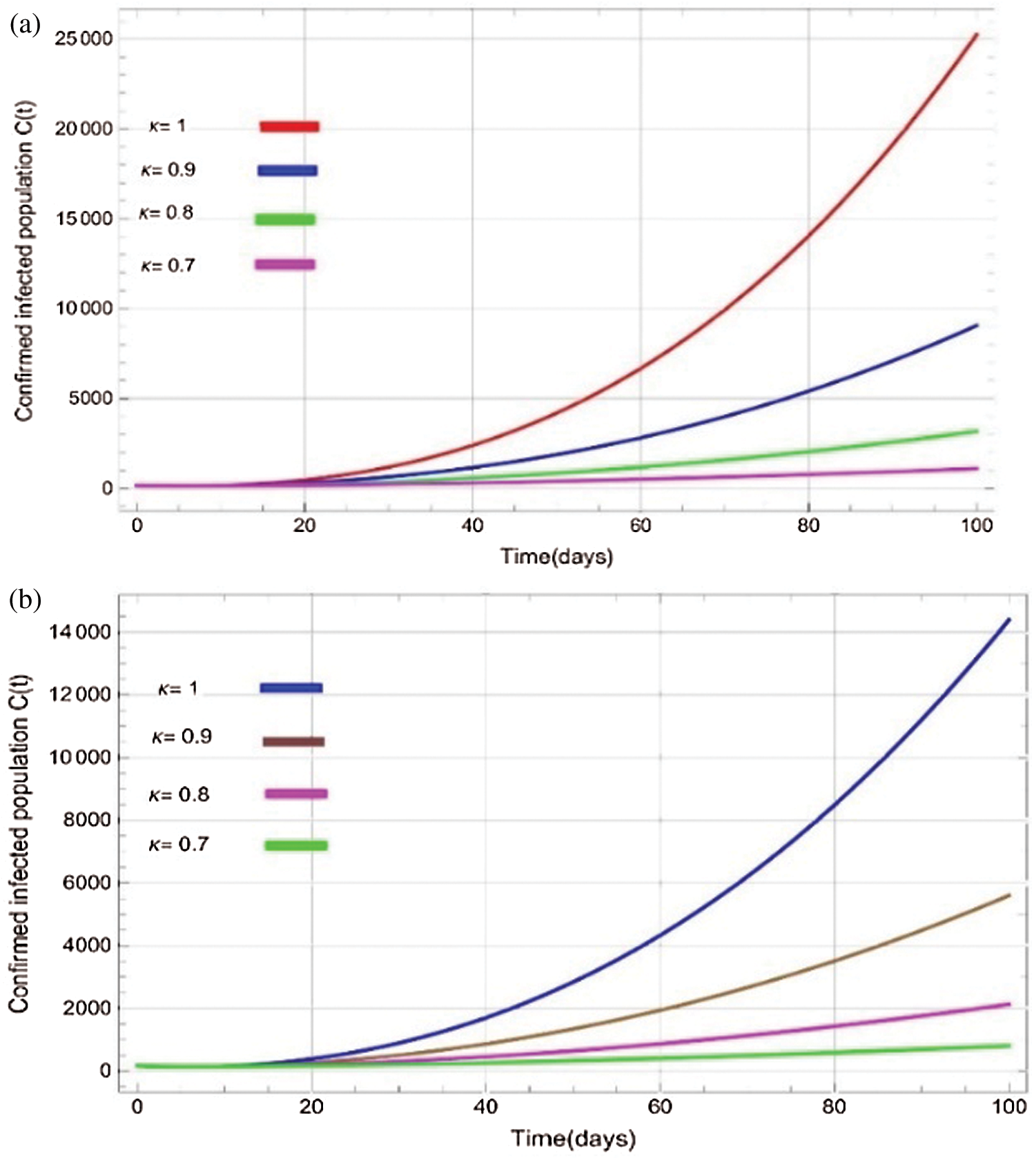
Figure 6: Plots of confirmed infected population for various values of  with respect to time t in days and different R0 [Fig. 6(a): R0 = 1.96, Fig. 6(b): R0 = 1.16]
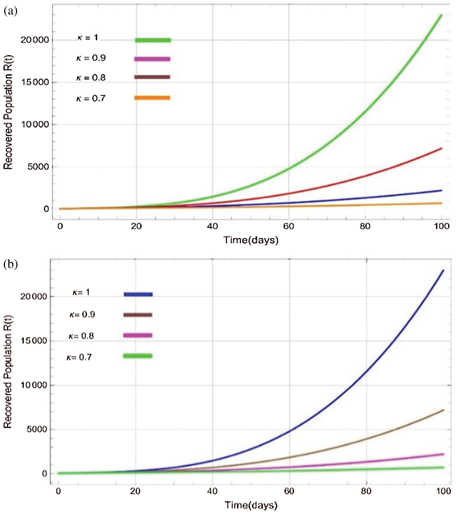
Figure 7: Plots of recovered population for various values of  with respect to time t in days and different R0 [Fig. 7(a): R0 = 1.96, Fig. 7(b): R0 = 1.16]
Also, Fig. 8a shows the comparison between estimated and actual number of cumulative cases of confirmed and quarantine population C(t) for data of available infection cases from April 1, 2020, till April 30, 2020 of Nigeria. This clearly shows that estimated and actual cases of infections are very near to each other. Fig. 8b shows the plots of total infected population in various compartments of model Eq. (1) versus time (days).

Figure 8: (a) Cumulative number of cases of infected population C(t) with respect to time(days) (b) Plot of total population in various classes of model versus time (days)
In this manuscript, we have analysed and examined transmission dynamics of COVID-19 infection formulated in terms of mathematical model based on fractional differential system. We have used Atangana–Baleanu fractional derivative operator to obtain existence criteria of solution of mathematical model for the operator. The numerical simulations are carried out using iterative Laplace transform method. The essential axioms of the proposed model have been studied to observe the biological and mathematical feasibility. Further, we have examined the sensitivity analysis by finding the basic reproductive number  which explains the significant of every biological parameter involved in the proposed model. Moreover, the local and global asymptotic stability conditions for the disease-free and endemic equilibrium are obtained which determines the conditions to stabilize the exponential spread of the disease. It is noted from this analysis, that parameters
  and
and  strengthen the outbreak of the infection at large extent and needs notable consideration to implement some control strategies to keep this under control. Towards the end all the hypothetical results are supported with the assistance of graphical portrayal by numerical investigation which would be beneficial for researchers to contemplate the dynamics of the COVID-19.
Funding Statement: The authors received no specific funding for this study.
Conflicts of Interest: “The authors declare that they have no conflicts of interest to report regarding the present study.”
1. COVID-19 Coronavirus Pandemic. (2020). [online]. Available: https://www.worldometers.info/coronavirus/#repro. [Google Scholar]
2. D. Wrapp, N. Wang and K. Corbett. (2020). “Cryo-EM structure of the 2019-nCoV spike in the prefusion Conformation,” Science, vol. 2, pp. 7–28. [Google Scholar]
3. A. B. Gumel. (2020). “Using mathematics to understand and control the 2019 novel coronavirus pandemic,” This Day Live, . Available: https://www.thisdaylive.com/index.php/2020/05/03/. [Google Scholar]
4. N. Zhu, D. Zhang and W. Wang. (2020). “A novel coronavirus from patients with pneumonia in China 2019,” New England Journal of Medicine, vol. 382, no. 8, pp. 727–733. [Google Scholar]
5. J. B. Aguilar, G. S. M. Faust, L. M. Westafer and J. B. Gutierrez. (2020). “A Model Describing COVID-19 Community Transmission Taking into Account Asymptomatic Carriers and Risk Mitigation,” medRxiv 2020.03.18.20037994. [Google Scholar]
6. Available: https://en.wikipedia.org/wiki/COVID-19_pandemic_in_Nigeria. [Google Scholar]
7. Nigeria Centre for Disease Control. Available: https://covid19.ncdc.gov.ng/. [Google Scholar]
8. T. M. Chen, J. Rui, Q. P. Wang, J. A. Cui and L. Yin. (2020). “A mathematical model for simulating the phase-based transmissibility of a novel coronavirus,” Infectious Diseases of Poverty, vol. 9, no. 1, pp. 24. [Google Scholar]
9. F. Ndaïrou, I. Area, J. J. Nieto and D. F. M. Torres. (2020). “Mathematical modelling of COVID-19 transmission dynamics with a case study of Wuhan,” Chaos, Solitons and Fractals, vol. 135, 109846. [Google Scholar]
10. C. Yang and J. Wang. (2020). “A mathematical model for the novel coronavirus epidemic in Wuhan China,” Mathematical Biosciences and Engineering, vol. 17, no. 3, pp. 2708–2724. [Google Scholar]
11. Y. Fang, Y. Nie and M. Penny. (2020). “Transmission dynamics of the covid-19 outbreak and effectiveness of government interventions: A data-driven analysis,” Journal of Medical Virology, vol. 2, pp. 6–21. [Google Scholar]
12. R. Xinmiao, Y. Liu, C. Huidi and F. Meng. (2020). “Effect of delay in diagnosis on transmission of COVID-19,” Mathematical Biosciences and Engineering, vol. 17, pp. 2725. [Google Scholar]
13. K. Mizumoto and G. Chowell. (2020). “Estimating risk for death from 2019 novel coronavirus disease, China, January–Febrary 2020,” Emerging Infectious Diseases, vol. 1, pp. 77–78. [Google Scholar]
14. Q. Lin, S. Zhao, D. Gao, Y. Lou, S. Yang. (2020). et al., “A conceptual model for the coronavirus disease 2019 (COVID-19) outbreak in Wuhan, China with individual reaction and governmental action,” International Journal of Infectious Diseases, vol. 2, no. 1, pp. 187–195. [Google Scholar]
15. B. Tang, X. Wang, Q. Li, N. L. Bragazzi, S. Tang. (2020). et al., “Estimation of the transmission risk of 2019nCoV and its implication for public health interventions,” Journal of Clinical Medicine, vol. 9, no. 2, pp. 462–464. [Google Scholar]
16. B. Ivorra, M. R. Ferrández, M. Vela-Pérez and A. M. Ramos. (2020). “Mathematical modeling of the spread of the coronavirus disease 2019 (COVID-19) considering its particular characteristics: The case of China,” Communication in Nonlinear Science and Numerical Simulation, vol. 1, pp. 4–19. [Google Scholar]
17. M. A. Khan and A. Atangana. (2020). “Modeling the dynamics of novel coronavirus (2019-nCov) with fractional Derivative,” Alexandria Engineering Journal, vol. 59, no. 4, pp. 2379–2389. [Google Scholar]
18. Y. Li, B. Wang, R. Peng, C. Zhou, Y. Zhan. (2020). et al., “Mathematical modeling and epidemic prediction of COVID-19 and its significance to epidemic prevention and control measures,” Annals of Infectious Disease and Epidemiology, vol. 5, no. 1, pp. 1052. [Google Scholar]
19. A. S. Shaikh, V. S. Jadhav, M. G. Timol, K. S. Nisar and I. Khan. (2020). “Analysis of the COVID- 19 pandemic spreading in India by an epidemiological model and fractional differential operator,” Preprints, vol. 2020, pp. 2020050266. [Google Scholar]
20. A. S. Shaikh, I. N. Shaikh and K. S. Nisar. (2020). “A mathematical model of COVID-19 using fractional derivative: Outbreak in India with dynamics of transmission and control,” Advances in Difference Equations, vol. 2020, no. 373, pp. 264. [Google Scholar]
21. X. Jiang, M. Coffee, A. Bari, J. Wang, X. Jiang. (2020). et al., “Towards an artificial intelligence framework for data-driven prediction of Coronavirus clinical severity,” Computers, Materials & Continua, vol. 63, no. 1, pp. 537–551. [Google Scholar]
22. B. R. Sontakke, A. S. Shaikh and K. S. Nisar. (2018). “Approximate solutions of a generalized Hirota-Satsuma coupled KdV and a coupled mKdV system with time fractional derivatives,” Malaysian Journal of Mathematical Sciences, vol. 12, no. 2, pp. 173–193. [Google Scholar]
23. B. R. Sontakke and A. Shaikh. (2016). “Approximate solutions of time fractional Kawahara and modified Kawahara equations by fractional complex transform,” Communications in Numerical Analysis, vol. 2, no. 2, pp. 218–229. [Google Scholar]
24. A. Shaikh, A. Tassaddiq, K. S. Nisar and D. Baleanu. (2019). “Analysis of differential equations involving Caputo-Fabrizio fractional operator and its applications to reaction-diffusion equations,” Advances in Difference Equations, vol. 2019, no. 1, pp. 178. [Google Scholar]
25. A. S. Shaikh and K. S. Nisar. (2019). “Transmission dynamics of fractional order Typhoid fever model using Caputo Fabrizio operator,” Chaos Solitons and Fractals, vol. 128, pp. 355–365. [Google Scholar]
26. S. Kumar, A. Kumar and D. Baleanu. (2016). “Two analytical methods for time-fractional nonlinear coupled Boussinesq-Burger’s equations arise in propagation of shallow water waves,” Nonlinear Dynamics, vol. 85, no. 2, pp. 699–715. [Google Scholar]
27. S. X. Wang, J. H. He, C. Wang and X. T. Li. (2018). “The definition and numerical method of final value problem and arbitrary value problem,” Computer Systems Science and Engineering, vol. 33, no. 5, pp. 379–387. [Google Scholar]
28. F. Peng, D. L. Zhou, M. Long and X. M. Sun. (2017). “Discrimination of natural images and computer generated graphics based on multi-fractal and regression analysis,” AEU: International Journal of Electronics and Communications, vol. 71, pp. 72–81. [Google Scholar]
29. D. P. Tian. (2018). “Particle swarm optimization with chaos-based initialization for numerical optimization,” Intelligent Automation and Soft Computing, vol. 24, no. 2, pp. 331–342. [Google Scholar]
30. K. M. Owolabi and A. Atangana. (2019). “Mathematical analysis and computational experiments for an epidemic system with nonlocal and non-singular derivative,” Chaos, Soliton and Fractals, vol. 1, no. 126, pp. 41–49. [Google Scholar]
31. K. M. Saad, D. Baleanu and A. Atangana. (2018). “New fractional derivatives applied to the Korteweg-de-Vries and Korteweg-de Vries-Burger’s equations,” Computational & Applied Mathematics, vol. 37, no. 6, pp. 5203–5216. [Google Scholar]
32. A. Atangana and D. Baleanu. (2016). “New fractional derivatives with non-local and non-singular kernel: Theory and application to heat transfer model,” Thermal Science, vol. 20, no. 2, pp. 763–769. [Google Scholar]
33. A. Atangana and K. M. Owolabi. (2018). “New numerical approach for fractional differential equations,” Mathematical Modelling of Natural Phenomena, vol. 13, no. 1, pp. 1–21. [Google Scholar]
34. K. M. Owolabi. (2018). “Numerical patterns in reaction-diffusion system with the Caputo and Atangana-Baleanu fractional derivatives,” Chaos, Solitons and Fractals, vol. 115, pp. 160–169. [Google Scholar]
35. B. Rahman, E. Sadraddin and A. Porreca. (2020). “The basic reproduction number of SARS-CoV-2 in Wuhan isabout to die out, how about the rest of the World,” Reviews in Medical Virology, vol. e2111, pp. 1–10. [Google Scholar]
36. COVID-19 Dashboard, Available: https://coronaworld.info/dashboard/. [Google Scholar]
37. C. Geller, M. Varbanov and R. E. Duval. (2012). “Human coronaviruses: Insights into environmental resistance and its influence on the development of new antiseptic strategies,” Viruses, vol. 4, no. 11, pp. 3044–3068. [Google Scholar]
38. The government of Wuhan homepage. Available: http://english.wh.gov.cn/. [Google Scholar]
 | This work is licensed under a Creative Commons Attribution 4.0 International License, which permits unrestricted use, distribution, and reproduction in any medium, provided the original work is properly cited. |