DOI:10.32604/cmc.2020.012706
| Computers, Materials & Continua DOI:10.32604/cmc.2020.012706 | |
| Article |
NURBS Modeling and Curve Interpolation Optimization of 3D Graphics
1School of Information and Communication Engineering, Nanjing Institute of Technology, Nanjing, 211167, China
2Jiangsu Key Laboratory of Advanced Numerical Control Technology, Nanjing Institute of Technology, Nanjing, 211167, China
3Department of informatics, University of Leicester, Leicester, LE1 7RH, UK
*Corresponding Author: Hao Zhu. Email: zhuhao@njit.edu.cn
Received: 10 July 2020; Accepted: 29 September 2020
Abstract: In order to solve the problem of complicated Non-Uniform Rational B-Splines (NURBS) modeling and improve the real-time performance of the high-order derivative of the curve interpolation process, the method of NURBS modeling based on the slicing and layering of triangular mesh is introduced. The research and design of NURBS curve interpolation are carried out from the two aspects of software algorithm and hardware structure. Based on the analysis of the characteristics of traditional computing methods with Taylor series expansion, the Adams formula and the Runge-Kutta formula are used in the NURBS curve interpolation process, and the process is then optimized according to the characteristics of NURBS interpolation. This can ensure accuracy, and avoid the calculation of higher-order derivatives. Furthermore, the hardware modules for the Adams and Runge-Kutta formulas are designed by using the parallel hardware construction technology of Field Programmable Gate Array (FPGA) chips. The parallel computing process using FPGA is compared with the traditional serial computing process using CPUs. Simulation and experimental results show that this scheme can improve the computational speed of the system and that the algorithm is feasible.
Keywords: NURBS modeling; interpolation; Adams; Runge-Kutta; FPGA
The Non-Uniform Rational B-Splines (NURBS) model was proposed by Piegl et al. [1]. This model provides a unified mathematical description method for analytic curves, analytic surfaces, free curves, and free surfaces. Due to its universality and simplicity of calculation, the NURBS model has become the only mathematical description method used in computer-aided design (CAD) to define product geometry. Having the NURBS curve interpolation function has become a key index for determining the performance of computer numerical control (CNC) systems [2]. There are many ways to describe the NURBS curve. One of the most commonly used is the parameter description [3].
2 NURBS Surface Generation Based on Triangle Mesh Model
2.1 Slicing and Layering of Triangle Mesh Model
3D reconstruction technology based on triangular patch is a classic reverse engineering technology. Reference [4] applied artificial neural network technology to the reconstruction of triangular patches. Reference [5] proposed a method of generating triangular patch model based on shape from silhouette technology. The research of slicing and layering technology based on the triangle mesh model has enjoyed many successes [6–9]. There are three categories of layered algorithms: The layered algorithm based on the location of triangle meshes, the layered algorithm based on the topological relationship of triangle meshes, and the layered algorithm based on out-of-core technology. In this paper, because the subsequent modeling requires an ordered point set, the layered algorithm based on the topological relationship of triangle meshes is used to obtain it. Reference [10] proposed a recursive slicing method based on the directed weighted graph. Reference [11] modified this method to improve the layering speed. In this improved method, a directed weighted sorting for the adjacent triangular patches was established. Using the triangular pyramid ABCD shown in Fig. 1 as an example, its four faces are numbered 0, 1, 2, and 3. Face 0 is the under-side triangular patch BCD. Face 1 is the left-side triangular patch ABD. Face 2 is the right-side triangular patch ACD. Face 3 is the front-side triangular patch ABC. The three angles of each triangular patch are defined as v0, v1, and v2. The subscript is defined as the number of the angle.
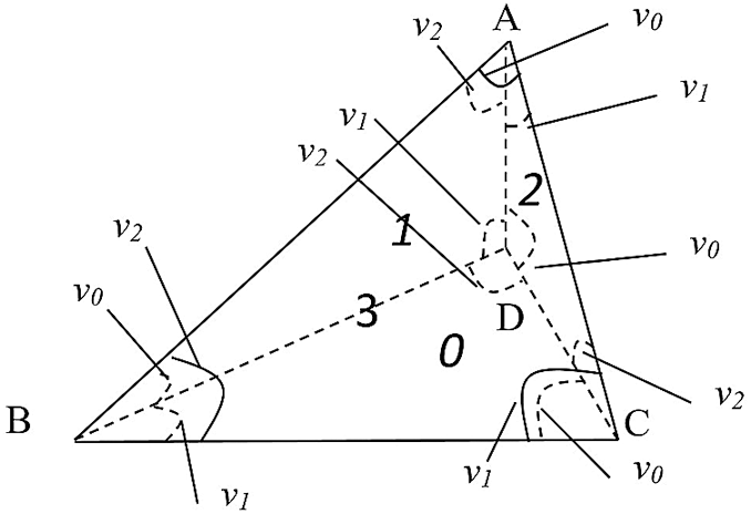
Figure 1: Weighted sorting of triangle meshes
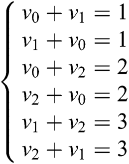
The information for each face includes its number and the three weights of the three edges. The weight of edge is defined as follows. For an edge of the current face, the weight is the sum of two angles’ numbers. These two angles satisfy the two following conditions: They are in the adjacent face (the face that shares the edge with the current face); and they are adjacent to the current face. As shown in Fig. 1, edge AB is the edge shared by face 3 (the current face) and face 1 (the adjacent face). The weight of the edge AB is the sum of the number of ∠BAD (v2) and the number of ∠ABD (v0), i.e., 2 + 0 = 2. The rules for adding angle numbers are shown in Eq. (1).
The directed weighted vector graph is shown in Fig. 2. The circles represent four triangular patches. The arrows point from the current face to the adjacent face. The value of the arrow indicates the weight.
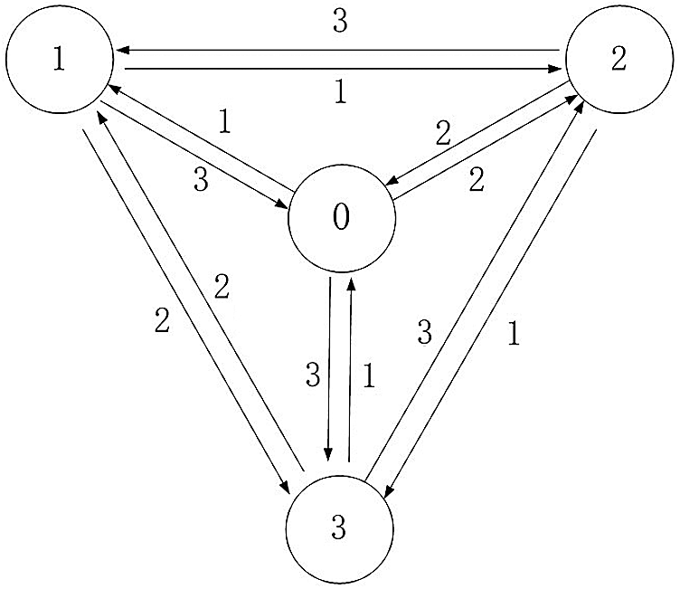
Figure 2: Directed weighted vector graph of triangular patches
According to the above definition, every edge of each triangle patch can be recorded. The information of the triangular patch can be stored in the linked list structure. Each triangular patch corresponds to a chain node. Every node member includes the triangular patch number, the normal vector, the division mark, and the vertex coordinate. In addition, each edge is a child node of the triangular patch node. Each child node member includes the number of the triangle patch that shares this edge, the weight of this edge, and the address of the next edge. According to this structure, each edge of each triangular patch can be found in order when the triangular mesh model is layered. If the current triangular patch has been layered, it can be marked at the same time.
The core process of triangle mesh model layering is to use a series of planes perpendicular to the z axis of the rectangular coordinate to intersect with the triangular patch and record the intersection point set. As shown in Fig. 3, the three vertices of the triangular patch are  ,
,  , and
, and  . The section plane intersects the triangular patch. The intersection point of the plane and the edge Q1Q2 is
  . The point satisfies Eq. (2):
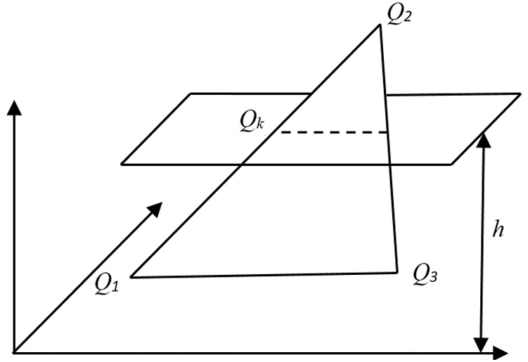
Figure 3: Schematic diagram of intersection of section plane and triangular patch
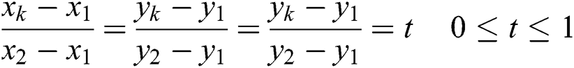
The coordinates of intersection point Qk can be obtained by solving Eq. (3).
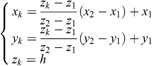
where h is the height of the current section plane.
As shown in Fig. 4, when the section plane intersects with each triangle patch, two intersections are obtained. For two adjacent triangle patches, the intersection of the section plane and the common edge produces the repeating node. In the link list node structure, the segmentation mark can be used to record the layered state of the triangular patch by the current section plane. The repeating node can be eliminated through the above state.
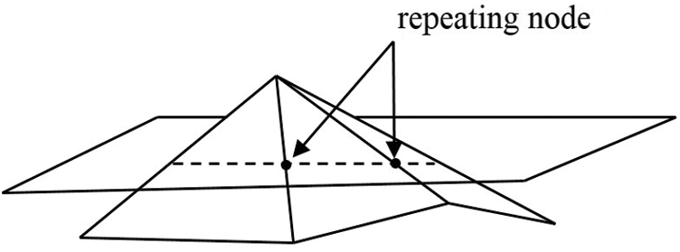
Figure 4: Repeating node of adjacent triangular patches
The layering algorithm is described as follows:
Step 1: Prescreen the triangle patch according to the Z coordinate of each triangle, and filter out the triangular patches that do not intersect with the current section plane.
Step 2: Weighted sort the remaining triangular patches to determine the order.
Step 3: Traverse each triangle in order of weight, and store the calculated intersection points in the chain list.
The resulting linked list data are the ordered intersection data.
2.2 NURBS Curve Reconstruction
As described in Section 2.1, a series of ordered intersection points can be obtained. Reference [1] presented a method of interpolating non-rational B-spline curves and surfaces based on the ordered data points. The algorithm of interpolating NURBS curve and surface can be designed based on this idea.
Set the interpolation object as a series of ordered data points Qk, k = 0,1,2…,n. It is necessary to create a p-th NURBS curve to interpolate these points. For the sake of simplicity, in the weight vector, let all  . If a parameter value
  is specified for each data point Qk, and a reasonable node vector
 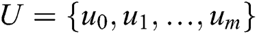 is designed, then Eq. (4) can be obtained.
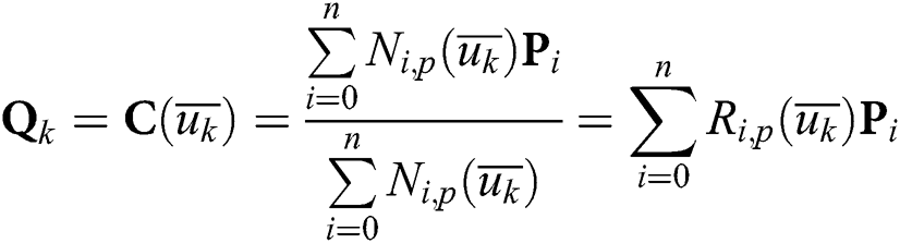
where 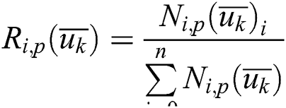
It can be seen that Eq. (4) is a system of linear equations with n + 1 control points Pt as the independent variable and matrix of (n + 1) × (n + 1) as the coefficient matrix.
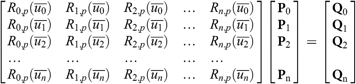
where Ri,p(u) can be calculated by the Cox-de Boor recurrence formula. Therefore, the key to solving this system of equations is how to select the appropriate parameter value  and the node vector U = {u0,u1,…um}. It is assumed that all of the parameters satisfy u ∈ [0,1]. Generally, the chord length parameter method can be used to select the parameter value.
2.3 NURBS Surface Interpolation
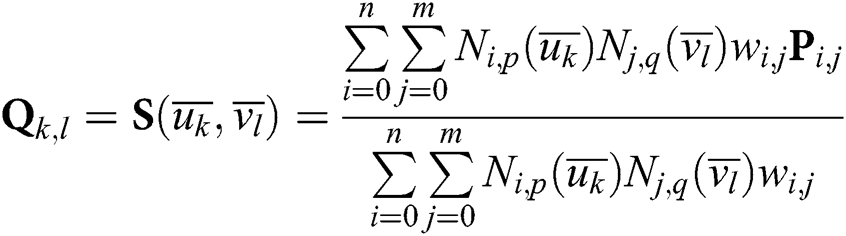
Suppose there are (n + 1) × (m + 1) data points Qk,l, k = 0,1,…n, l = 0,1,…,m. Surface interpolation creates a non-rational (p, q) degree B-spline surface to interpolate these points.
Similar to NURBS curves, it is necessary to calculate the reasonable parameters  , node vectors U and V at first. Using
  as an example, the algorithm is as follows:
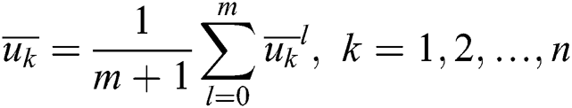
Step 1: Calculate the mean value  in V direction.
Step 2: Average all  in U direction.
The algorithm of solving  is similar to that of
  . Once
  and
and  are obtained, the node vectors U and V can be obtained. For the control points:
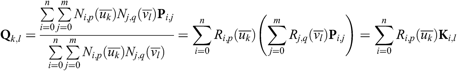
where
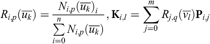
It can be found that Eq. (8) is the interpolation equation for curve interpolation of data point Qk,j (k = 0,1,…,n) in the U direction. Ki,l is the isoparametric curve control point of surface S(u,v) when  . Similarly, when i is fixed and l changes, Eq. (9) is an interpolation equation for data point Ki,l (l = 0,1,…,m). Pi,j on the right side of the equation is the control point to be solved. Therefore, the algorithm to solve the control point is as follows:
Step 1: In the direction of U, solve the curve interpolation equation according to the parameter  and the data point Qk,j (k = 0,1,…,n), then get Ki,l.
Step 2: In the direction of V, solve the curve interpolation equation according to the parameters  and the data point Ki,l (l = 0,1,…,m), then get Pi,j.
3 NURBS Curve Interpolation Optimization Method
3.1 Method of Finding the Position Parameter Based on the Optimized Adams Algorithm
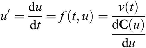
NURBS interpolation is the process of calculating the tool position Pj+1 = {x(uj+1), y(uj+1), z(uj+1)} after an interpolation cycle based on the federate v(t), the interpolation cycle , and the current tool position Pj = {x(uj), y(uj), z(uj)}. In the NURBS parameter curve C(u), the position parameter uj+1, which is after an interpolation period, needs to be computed based on the current position parameter uj in the parameter domain and the feed speed v(t) in the track domain. This process is commonly implemented by using the Taylor series expansion algorithm [12].
The disadvantage of the Taylor series expansion method is that if we want more accurate results, we need higher-order Taylor series expansion. That is to say, we need to compute the higher-order derivatives of the NURBS curves, which is a complex process. However, reducing the Taylor series expansion order will reduce the computational accuracy. In view of this problem, we can design an optimization algorithm based on the Adams formula and calculate uj+1 quickly.
The Adams formula is a numerical integration method. Its basic purpose is to solve general ordinary differential equations such as Eq. (10) with a linear multi-step method [13].
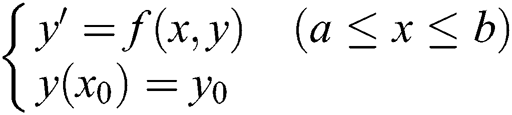
In this equation, the step size is h, let xn = x0 + nh (n = 1, 2, …).
Once the function value y(xn) of the node xn is obtained according to a certain recursion principle, Eq. (10) can be solved.
In the Adams algorithm, take the slope values of the first few steps of y(x). The weighted average of these values is taken as the slope value to estimate the current function value. When the selected point is the node before the current point, it is the explicit Adams format. When the selected points include the node before the current point and after the current point, it is the implicit Adams format. The explicit and implicit Adams formats are shown as Eqs. (11) and (12).

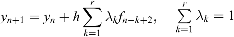
where 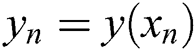 ,
,  . r is the order of the Adams formula.
The common three-step fourth-order Adams explicit formula is shown in Eq. (13).

where h is the step value and the truncation error is O(t5).
Applying the idea of an ordinary differential equation to the NURBS curve model, the following settings can be made:
Make interpolation cycle  , parameter node
 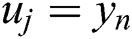 , then:
According to the above settings, and referring to the most commonly used three-step four-order Adams formula, the method of calculating uj+1 is shown in Eq. (15).

It can be seen from Eq. (15) that for the same order Adams algorithm and Taylor series expansion algorithm, their truncation error is the same. Using the fourth-order algorithms as an example, both of them are O(t5). By comparison, the Adams explicit formula avoids the high-order derivative calculation encountered by Taylor series expansion. At the same time, it can greatly improve the operation speed. However, the first derivative still exists in the Adams formula. Therefore, we continue to optimize the algorithm by replacing the derivative with difference quotient of C(u).
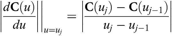
Take Eqs. (14) and (16) into Eq. (15), we can obtain:

It can be seen from Eq. (17) that the value uj+1 of the position parameter can be calculated by the current position parameter and the four position parameters uj, uj-1, uj-2, uj-3 and uj-4 before the current position. At the same time, the previous multi-step position parameters uj, uj-1, uj-2…… are needed to calculate the current position parameter uj+1 by the Adams formula. The higher the order is, the more that pre-order position parameters are needed. Therefore, on the premise that the truncation error is small enough, the system cannot start itself only by the Adams algorithm. To solve this problem, we need to use the linear single step algorithm to obtain the initial n position parameters. Of the many single-step algorithms, the Runge-Kutta algorithm is a calculation method with high accuracy [14]. In this paper, the algorithm is used to achieve the self-starting of the system.
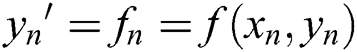
The Runge-Kutta algorithm evolved from the Euler algorithm. For the first-order ordinary differential equation shown in Eq. (10), we can see that
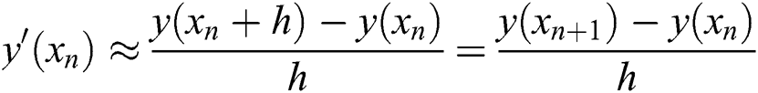
Therefore, let yn = y(xn), yn+1 = y(xn+1), there is 
Eq. (18) is the Euler formula. f(xn, yn) is the slope at point xn. Because the function value of the latter step is predicted only by the single point slope, the error of the Euler formula is large. The idea of the Runge-Kutta algorithm is to take several points in the interval [xn, xn+1] and take the weighted average value of its slope as the function value after the average slope prediction. This gives it higher accuracy.
The commonly used fourth-order Runge-Kutta formula is shown in Eq. (19).
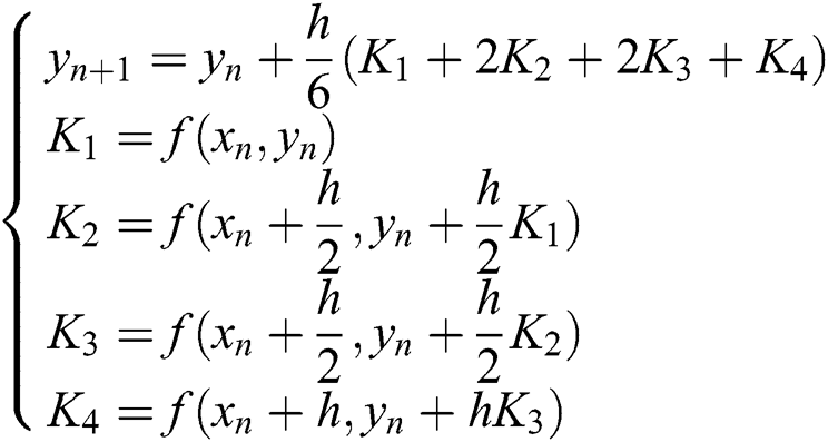
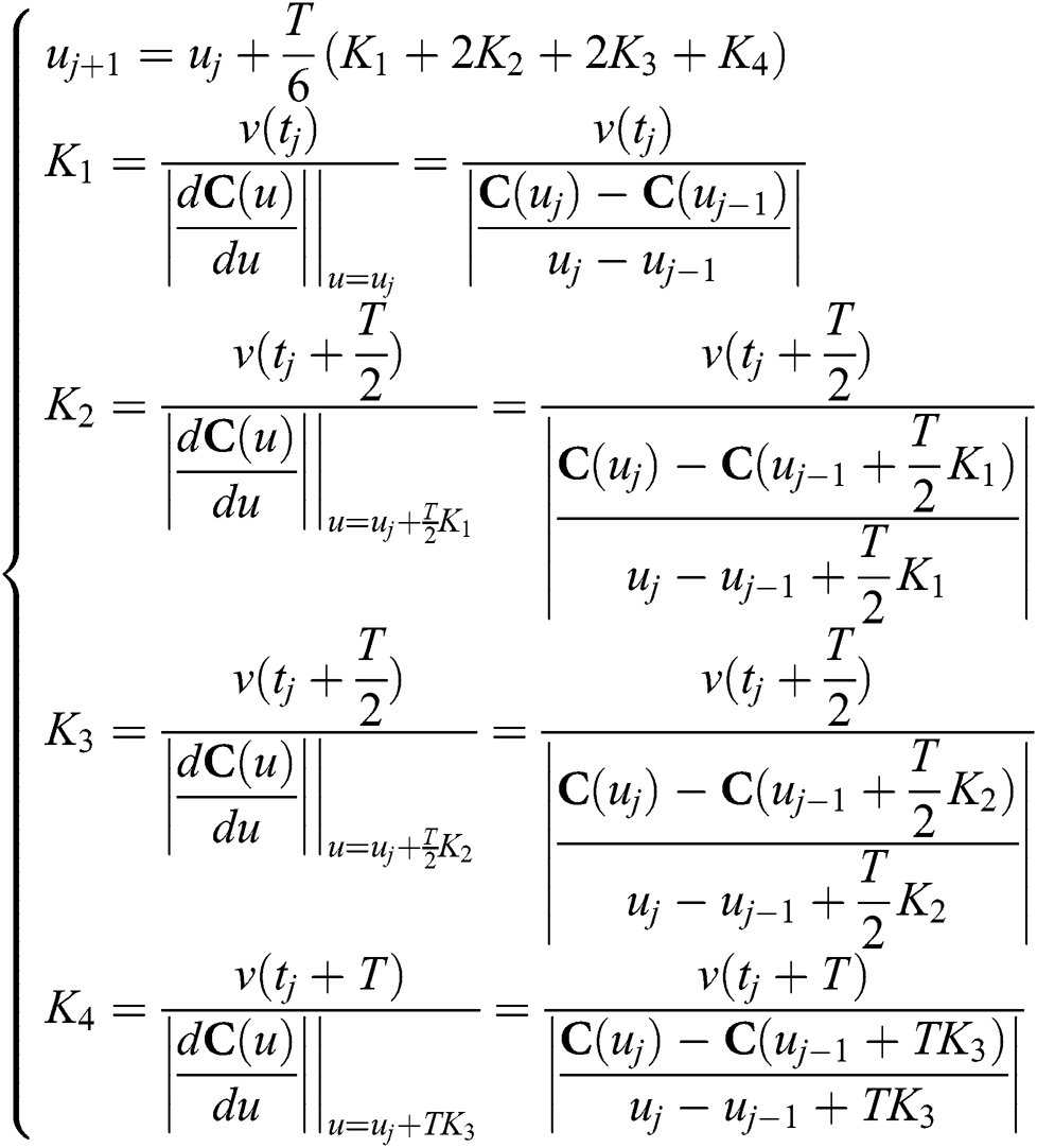
By using the definitions of Eq. (14) and substituting the derivative with difference quotient, the fourth-order Runge-Kutta formula can be applied to the NURBS curve model to obtain Eq. (20).
According to the principle of the Runge-Kutta formula, the parameters uj+1 of NURBS curve can be calculated by using Eq. (20) recursively. However, by comparing Eqs. (20) and (17), it can be seen that the Runge-Kutta method needs to use the recursive operation, which requires a large amount of calculation. Therefore, according to the Runge-Kutta method, the first four position parameters u1, u2, u3 and u4 are calculated by Eq. (20). According to the Adams method, with a relatively small amount of calculation, the rest of the position parameters are calculated by Eq. (17). Of these, the calculation method of the feed speed v(t) can refer to the relevant discussion and calculation [15].
3.2 Hardening Implementation of Parallel Computing
It can be seen from the previous description that, for a NURBS curve with n parameters, the Runge-Kutta formula of 4 times and the Adams formula of n−4 times need to be calculated. If the conventional CPU such as a microcontroller unit (MCU) or advanced reduced instruction set machine (ARM) is used for calculation, using the fourth-order Runge-Kutta and Adams formula as an example, the next parameter needs to be obtained by 8 times of serial calculation of C(u). This is undoubtedly a bottleneck for real-time CNC machining processes. For this type of operation, using a large number of logic units integrated in the FPGA to build parallel computing logic can greatly improve the system operation speed. At the same time, after the FPGA program is hardened, the calculation process is completed by hardware digital logic. Compared with the process of executing a software program with the CPU, the speed will be greatly improved [16–18].
The hardware structure of implementing the Runge-Kutta and Adams formulas by parallel computing is shown in Figs. 5 and 6.
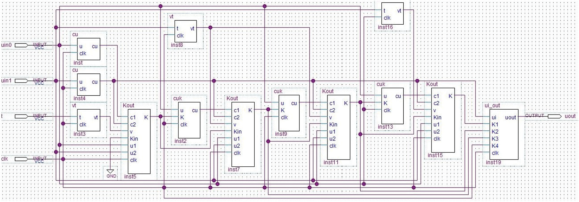
Figure 5: Parallel computing module structure of the Runge-Kutta formula
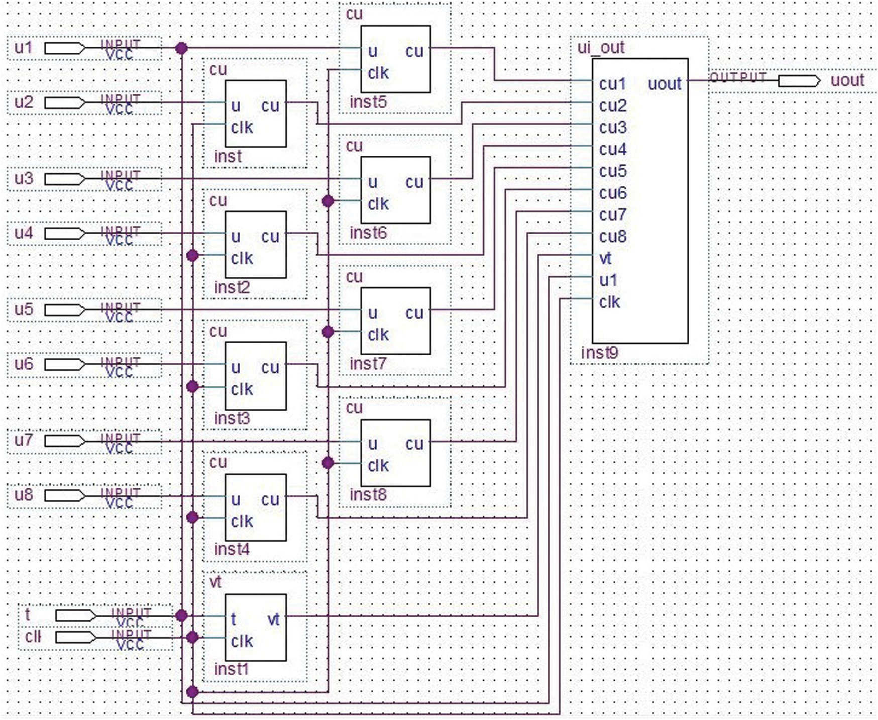
Figure 6: Parallel computing module structure of the Adams formula
In Figs. 5 and 6, module cu is used to calculate C(u), module vt is used to calculate v(t), module ui_out is used to calculate the next position parameter ui+1, module cuk is used to calculate C(uj-1 + (T/2)Ki), and module Kout is used to calculate Ki. The calculation of module cu requires multiple clock cycles, which will take up most of the calculation time, while the Kout and ui_out modules can be calculated in one clock cycle by using the parallel multiplier and divider in the FPGA. If the clock period is set as Δt and the calculation time of the module cu is T, the parallel structure calculation of the Adams and Runge-Kutta formulas require T + Δt and 4T + 5Δt, respectively. Considering T >>Δt, for NURBS curves with n parameters, the times for parallel and serial calculation are shown in Tab. 1. It can be seen that the parallel computing will greatly shorten the computing time.
Table 1: Time comparison between serial computing and parallel computing
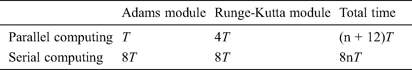
Fig. 7 shows, from left to right, the point cloud model, the triangular patch model, the NURBS layered curve model, and the surface reconstruction model of the target.
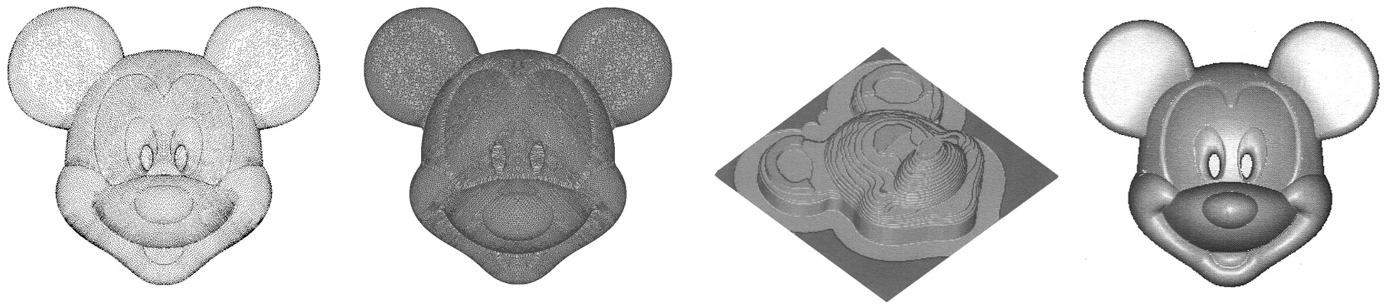
Figure 7: NURBS modeling of a 3D image
To verify the correctness of the interpolation algorithm, this paper simulates the quadratic NURBS curve in MATLAB. The parameters of NURBS curve are as follows: Degree p = 2. The control points are P0(1,2), P1(1.5,1), P2(3,3), P3(4,3.5), P4(5,3), P5(6.5,1), and P6(7,2). Node vector U = {0,0,0,1/5,2/5,3/5,4/5,1,1,1}, weight W = {1,1,1,1,1,1,1}. The interpolation path is shown in Fig. 8. The processing parameters are as follows: interpolation period T = 1 ms, maximum feed speed vm = 4 mm/s, and initial speed vs = 0 mm/s. Maximum bow height error ε = 1 μm. Reference [15] introduced a model to calculate v(t). The relationship between the position parameter u and the processing time is shown in Fig. 9. The relationship between the step value Δu of u and the processing time is shown in Fig. 10. As the curvature radius of the machining path changes, the step value of the position parameter also changes, so the position parameter does not have a linear relationship with the machining time.
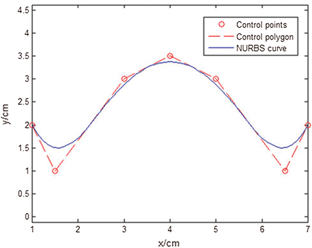
Figure 8: NURBS path to be machined
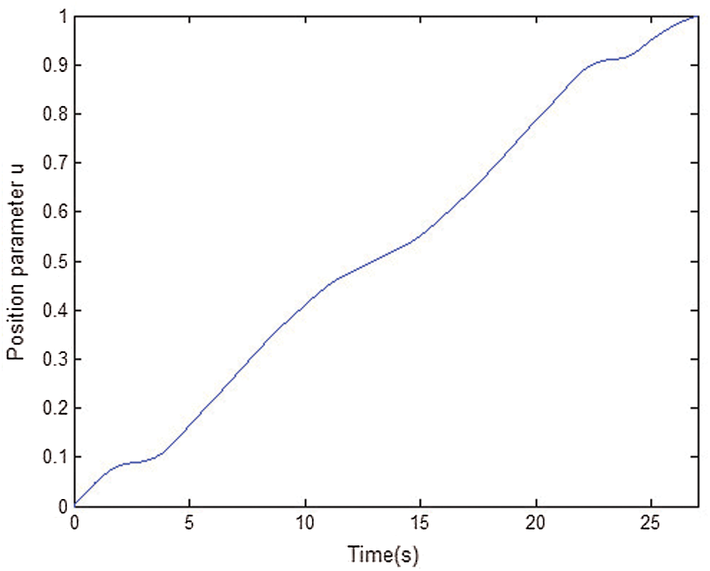
Figure 9: Position parameter u
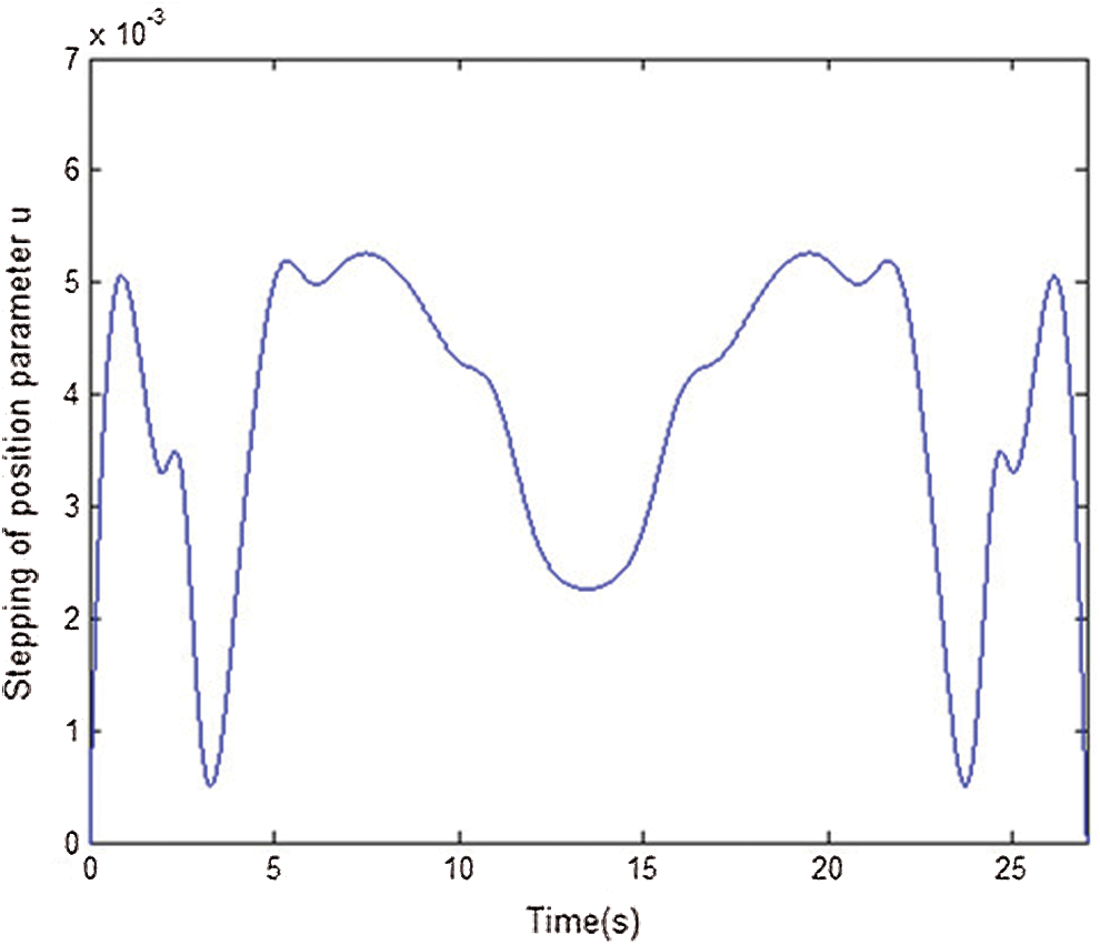
Figure 10: Position parameter step value
Next, the time consumption of serial computing and parallel computing was studied. The FPGA model was ep2c8q208, the system clock was 50 MHz, and then the clock cycle Δt = 0.02 μs, with the computing time of cu T = 205 μs. The time required to calculate the first 12 position parameters uj+1 by serial calculation and parallel calculation is shown in Fig. 11. It can be seen that the time to calculate the position parameters uj+1 by serial calculation was more than the actual interpolation period of the machine tool, and therefore, it cannot meet the real-time requirements of machining. However, the time for the parallel calculation was far less than the actual interpolation period of the machine tool.
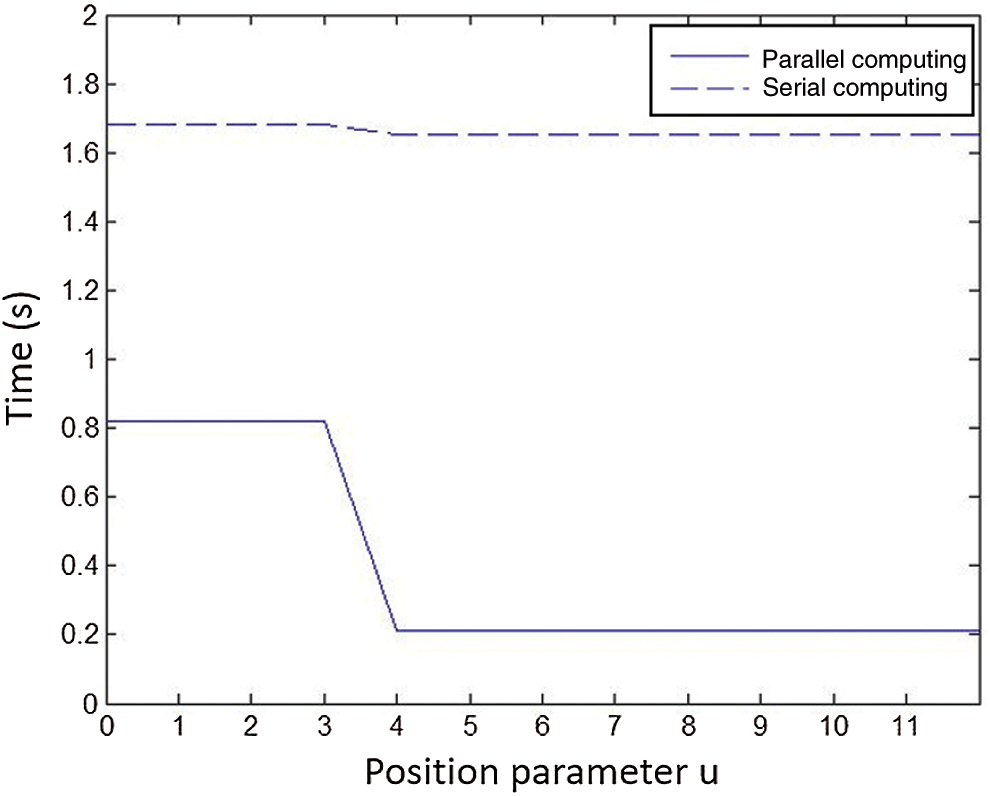
Figure 11: Position parameter calculation time
This paper introduces a method of NURBS surface reconstruction based on triangle mesh layering. Based on an analysis of existing algorithms, the Adams and Runge-Kutta algorithms were introduced into the process of NURBS interpolation, thereby avoiding the complex high-order calculation of the NURBS curve and reducing the amount of calculation from the perspective of the software algorithm. At the same time, the hardware parallel computing module was designed based on the FPGA parallel hardware architecture. This module replaces the common software computing mode based on the CPU and improves the computing speed. The analysis results show that the algorithm proposed in this paper can correctly obtain the position parameters of NURBS curve. Therefore, when combined with the hardware structure of parallel computing, this method can improve the real-time performance of the system.
Funding Statement: This work was supported by Natural Science Foundation of Universities in Jiangsu Province (Grant No. 16KJA460001), Creation Foundation Project of Nanjing Institute of Technology (Grant No.: ZKJ201611).
Conflicts of Interest: The authors declare that they have no conflicts of interest to report regarding the present study.
1. L. Peigl and W. Tiller. (1995). The NURBS Book. Berlin, Germany: Springer Press. [Google Scholar]
2. S. Wang. (2013). “The evaluation and correction of the reconstructed NURBS surface smoothing and accuracy,” Sensors and Transducers, vol. 161, no. 12, pp. 395–400. [Google Scholar]
3. D. Fazanaro, P. H. J. Amorim, T. Moraes, J. V. L. D. Silva and H. Pedrini. (2016). “NURBS parameterization for medical surface reconstruction,” Applied Mathematics, vol. 7, no. 2, pp. 137–144. [Google Scholar]
4. E. Yavuz and R. Yazici. (2019). “A dynamic neural network model for accelerating preliminary parameterization of 3D triangular mesh surfaces,” Neural Computing & Applications, vol. 31, no. 8, pp. 3691–3701. [Google Scholar]
5. W. Phothong, T. C. Wu, J. Y. Lai, W. D. Wang, Y. Liao. (2017). et al., “Fast and accurate triangular model generation for the shape-from-silhouette technique,” Computer-Aided Design and Applications, vol. 14, no. 4, pp. 436–449. [Google Scholar]
6. L. F. Leidinger, M. Breitenberger, A. M. Bauer, S. Hartmann, R. Wüchner. (2019). et al., “Explicit dynamic isogeometric B-rep analysis of penalty-coupled trimmed NURBS shells,” Computer Methods in Applied Mechanics and Engineering, vol. 351, pp. 891–927. [Google Scholar]
7. L. Gao, Y. Li, W. J. Li and Q. H. Zhao. (2017). “Combining the delaunay triangular mesh for image segmentation,” Journal of Signal Processing, vol. 33, no. 10, pp. 1393–1403.
8. D. Z. Sun, C. Z. Zhu and Y. R. Li. (2010). “Fast slicing algorithm for triangular mesh model,” Journal of Beijing University of Aeronautics and Astronautics, vol. 36, no. 3, pp. 279–282.
9. S. Joshi and Z. Y. Zhang. (2015). “An improved slicing algorithm with efficient contour construction using STL files,” International Journal of Advanced Manufacturing Technology, vol. 80, no. 5, pp. 1347–1362. [Google Scholar]
10. Y. Z. Ma, W. J. Liu and Y. T. Dong. (2003). “Study of slicing algorithm based on recurvsion and searching direct graph with weight,” China Mechanical Engineering, vol. 14, no. 14, pp. 1221–1224. [Google Scholar]
11. P. Z. Wen, W. M. Huang and C. K. Wu. (2008). “Modified fast algorithm for STL file slicing,” Computer Applications, vol. 28, no. 7, pp. 1766–1768. [Google Scholar]
12. A. Schollmeyer and B. Froehlich. (2018). “Efficient and anti-aliased trimming for rendering large NURBS models,” IEEE Transactions on Visualization and Computer Graphics, vol. 25, no. 3, pp. 1489–1498. [Google Scholar]
13. D. A. Voss and A. Q. M. Khaliq. (2015). “Split-step Adams-Moulton Milstein methods for systems of stiff stochastic differential equations,” International Journal of Computer Mathematics, vol. 92, no. 5, pp. 995–1011. [Google Scholar]
14. F. Rabiei, F. A. Hamid, N. M. Lazim, F. Ismail and Z. A. Majid. (2019). “Numerical solution of volterra integro-differential equations using improved Runge-Kutta methods,” Applied Mechanics and Materials, vol. 892, no. 6, pp. 193–199. [Google Scholar]
15. H. Zhu, J. N. Liu, A. K. Yang and M. L. Wang. (2013). “Fast interpolation scheme for NURBS curves based on fractional power polynomial,” China Mechanical Engineering, vol. 24, no. 23, pp. 3159–3163. [Google Scholar]
16. Z. Liu, X. A. Wang, C. J. Sun and K. Lu. (2019). “Implementation system of human eye tracking algorithm based on FPGA,” Computers, Materials & Continua, vol. 58, no. 3, pp. 653–664. [Google Scholar]
17. D. Silva, L. M. D. Torquato, M. F. Fernandes and A. C. Marcelo. (2019). “Parallel implementation of reinforcement learning Q-learning technique for FPGA,” IEEE Access, vol. 7, pp. 2782–2798.
18. C. Wang, J. Mao, T. Leng and Z. Y. Zhuang. (2017). “Efficient acceleration for total focusing method based on advanced parallel computing in FPGA,” International Journal of Acoustics and Vibration, vol. 22, no. 4, pp. 536–540. [Google Scholar]
 | This work is licensed under a Creative Commons Attribution 4.0 International License, which permits unrestricted use, distribution, and reproduction in any medium, provided the original work is properly cited. |