Computers, Materials & Continua DOI:10.32604/cmc.2020.012763
Article

Efficient Flexible M-Tree Bulk Loading Using FastMap and Space-Filling Curves

Woong-Kee Loh*

Department of Software, Gachon University, Seongnam, 13120, South Korea
*Corresponding Author: Woong-Kee Loh. Email: wkloh2@gachon.ac.kr
Received: 11 July 2020; Accepted: 09 August 2020

Abstract: Many database applications currently deal with objects in a metric space. Examples of such objects include unstructured multimedia objects and points of interest (POIs) in a road network. The M-tree is a dynamic index structure that facilitates an efficient search for objects in a metric space. Studies have been conducted on the bulk loading of large datasets in an M-tree. However, because previous algorithms involve excessive distance computations and disk accesses, they perform poorly in terms of their index construction and search capability. This study proposes two efficient M-tree bulk loading algorithms. Our algorithms minimize the number of distance computations and disk accesses using FastMap and a space-filling curve, thereby significantly improving the index construction and search performance. Our second algorithm is an extension of the first, and it incorporates a partitioning clustering technique and flexible node architecture to further improve the search performance. Through the use of various synthetic and real-world datasets, the experimental results demonstrated that our algorithms improved the index construction performance by up to three orders of magnitude and the search performance by up to 20.3 times over the previous algorithm.

Keywords: M-tree; metric space; bulk loading; FastMap; space-filling curve

1  Introduction

Many recent database applications deal with objects that are difficult to represent as points in a Euclidean space. Examples include the applications of unstructured multimedia objects such as images, voices, and texts [1–3], as well as those dealing with points of interest (POIs) in road networks [4–6]. These applications define the appropriate distance (or similarity) functions between two arbitrary objects, and the complexity of computing the distances is often much higher than that of computing distance in a Euclidean space. For example, in a road network application, the distance between two objects (vertices) is defined as the sum of the weights of the edges composing the shortest path between the objects. The complexity of Dijkstra’s algorithm, which has been widely used for finding the shortest path, is as high as 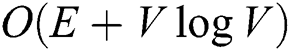, where E and V are the numbers of edges and vertices, respectively.

A metric space is formally defined as a pair , where is a domain of objects and is a distance function with the following properties:

1) (symmetry)

2) 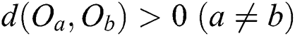and (non-negativity)

3) (triangle inequality)

The M-tree [7] is a dynamic index structure that facilitates an efficient search for objects in a metric space [8,9]. As the size of datasets used in recent applications continues to increase, it is crucial to construct and apply an indexing structure efficiently. Because it is highly inefficient and expensive to insert many objects into an index structure individually and sequentially, studies have been conducted on the bulk loading of large datasets in an M-tree [10–12]. However, because previous algorithms have involved excessive distance computations and disk accesses, they perform poorly in terms of their index construction and search capability.

Many recent metric space applications deal with highly dynamic datasets. For example, in road network applications, traffic situations change continuously owing to vehicle movements, unexpected accidents, and construction projects, etc. [13,14]. For such applications, it is crucial to quickly reorganize the indexes to reflect any changes in the datasets. When significant changes occur in a dataset as in road network applications, bulk loading is advantageous compared to updating almost the entire index. Moreover, many recent applications support various complicated queries, along with traditional proximity queries (range and k-NN queries). Examples include aggregate nearest neighbor (ANN) and flexible aggregate nearest neighbor (FANN) queries in road networks [6,14]. Studies have been recently conducted on the efficient processing of various queries including ANN and FANN using the M-tree [4,5].

In this study, we propose two efficient M-tree bulk loading algorithms that overcome the weaknesses of the previous algorithms. Our algorithms minimize the number of distance computations and disk accesses using FastMap [15] and a space-filling curve [16], thereby significantly improving the index construction and search performance. FastMap is a multidimensional scaling (MDS) method [17,18] that maps every object in a metric space into a point in a -dimensional Euclidean space such that the relative distances are maintained as much as possible. As mentioned above, because the cost of distance computations in a Euclidean space is much lower than that in a metric space, FastMap helps improve the index construction and search performance. The space-filling curve is used to define a total order among -dimensional points such that nearby -dimensional points are closely ordered. The one-dimensional sequence of ordered points is partitioned to form groups of nearby objects, and each group is stored in an M-tree node.

Our second algorithm is an extension of the first. It incorporates a partitioning clustering technique [19] and flexible node architecture to further improve the search performance. The clustering technique helps gather nearby objects and thereby minimize the size of the regions of object groups. The smaller region also reduces intersections with the search range, resulting in an improved search performance. The flexible node architecture is an adaptation of the concept of X-tree supernodes [20] composed of multiple contiguous disk pages, which are generated when it is anticipated to be beneficial to avoid splitting into a few nodes for a better search performance.

We compared the performance of our algorithms and the previous algorithm proposed by Ciaccia et al. [10] through experiments using synthetic and real-world datasets. The synthetic datasets were composed of objects in eight Gaussian clusters in a Euclidean space. For various dataset sizes (N) and dimensions (d), we compared the elapsed execution time and the number of distance computations and disk accesses for both index construction and k-nearest neighbor (k-NN) search. The results showed that our algorithms improved the index construction performance by up to three orders of magnitude over the previous algorithm. In particular, our second algorithm achieved a 20.3-fold improvement in the search performance. The real-world datasets were road networks (graphs) of various sizes obtained from the District of Columbia and five states in the United States. We conducted the experiments using these datasets in the same manner as the experiments using the synthetic datasets. The results demonstrated that our algorithms also improved the index construction performance by up to three orders of magnitude and that our second algorithm improved the search performance by up to 2.3 times.

The remainder of this paper is organized as follows. Section 2 describes the architecture of the M-tree and previous M-tree bulk loading algorithms. Sections 3 and 4 provide the details regarding our bulk loading algorithms. Section 5 describes the results of the experiments comparing the performance of index construction and k-NN search using various datasets. Finally, Section 6 concludes this paper.

2  Related Work

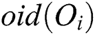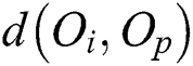The M-tree has a multilevel balanced tree structure similar to the R-tree [21]. Fig. 1a shows the structure of an M-tree leaf node entry, which corresponds to an object in the dataset. In the figure, is the feature value(s) representing ; is the object ID of ; and is the distance between and the parent object . The parent object is an object that represents all objects in the same leaf node and is determined using Eq. (1).

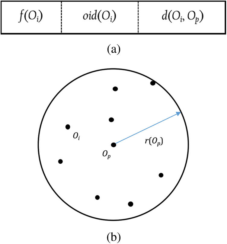
Figure 1: M-tree leaf node. (a) Leaf node entry. (b) Region corresponding to a leaf node

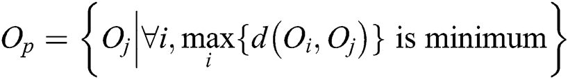
A leaf node is represented as a circular region centered by with radius = . This region is minimized to reduce the intersection with the query range based on a query object Q and, thus, to improve the search performance by avoiding access to unnecessary nodes. Fig. 1b shows a leaf node represented as a region containing all objects and a parent object . If an object that satisfies Eq. (1) were found in the Euclidean space, it would be close to the center of all objects in the leaf node. However, unlike in a Euclidean space, the concept of “center” is not defined in the metric space.

Fig. 2a shows the structure of an M-tree non-leaf node entry, which corresponds to a leaf or non-leaf node R in an M-tree. In the figure, indicates the feature value(s) representing the routing object ; is the radius, which is called the covering radius; is the pointer to the sub-tree rooted by R corresponding to the entry; and is the distance between and the parent object . The routing object is chosen as the parent object of the node R corresponding to the entry. The parent object in a non-leaf node, similar to that in a leaf node, is an object that represents all entries in the same node and is determined as a routing object satisfying Eq. (2).

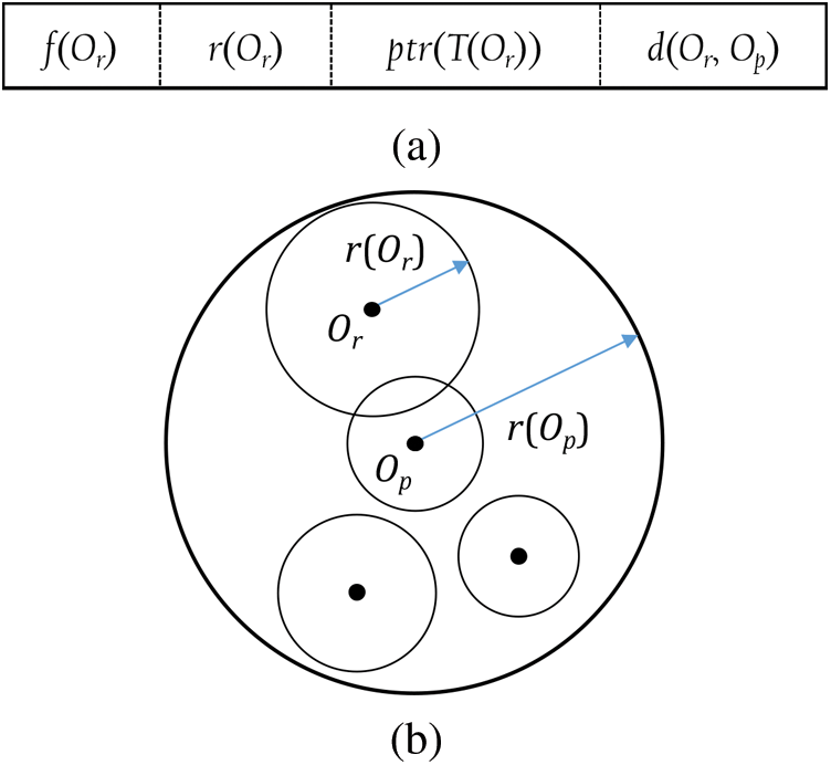
Figure 2: M-tree non-leaf node. (a) Non-leaf node entry. (b) Region corresponding to a non-leaf node

A non-leaf node is also represented as a circular region centered by with radius = . Fig. 2b shows a non-leaf node represented as a region containing the regions of R and a parent object . The leaf and non-leaf nodes of an M-tree are typically saved in a disk page of 4 KB size similarly to other index structures.

The first M-tree bulk loading algorithm, which is abbreviated as BulkLoad herein, was proposed by Ciaccia and Patella [10]. In BulkLoad, k arbitrary sample objects (i = 1..k) are initially extracted from a dataset of size N, and each of the remaining objects is assigned to the nearest sample object, thereby creating k sample sets . Then, for each sample set, the same task is recursively conducted to create a sub-tree . Finally, an M-tree is constructed by creating a root node containing the entries corresponding to all root nodes R of the k sub-trees. In this algorithm, to create the initial k sample sets, distance computations of complexity have to be performed. This task has to be recursively conducted until all leaf nodes are created in each sample set, that is, all the lowest level sub-sample sets have no more than M objects. Thus, assuming an even distribution of objects, the complexity of the entire algorithm is 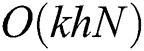, where h is the height of the M-tree. By setting k = M, because 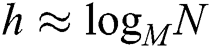, the complexity of the algorithm is 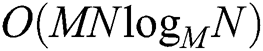, where M is the maximum number of entries in a leaf or non-leaf node 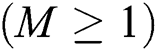. The problem of BulkLoad is that the final M-tree is highly dependent on the initial and subsequent selection of the sample objects. Moreover, because the objects among the sample sets are not evenly distributed, the final tree is not balanced. To solve this problem, BulkLoad redistributes the objects across sample sets; however, this incurs a large number of disk accesses, thereby significantly degrading the overall performance [11].

Sexton et al. [12] proposed an M-tree bulk loading algorithm to enhance the search performance. This algorithm generates an M-tree node by gathering nearby objects using a hierarchical clustering technique. However, the algorithm performs distance computations for all possible object pairs to find the closest pair, and the complexity is . Because this task should be repeated until all objects are contained in clusters, the complexity of the entire algorithm is , which is extremely high. Sexton et al. [12] compared the search performance of their algorithm only with the sequential insertion version of the M-tree generation algorithm [7] but not with BulkLoad [10]. Qiu et al. [11] proposed a parallel extension of BulkLoad. However, this algorithm merely splits the tasks of BulkLoad among multiple cores; thus, the disadvantages of BulkLoad persist. In particular, a significant degradation in the performance occurs not only by saving the intermediate results for object redistribution in a disk, but also due to I/O conflicts occurring when several threads try to access the same intermediate results simultaneously [11].

As described above, previous M-tree bulk loading algorithms apply excessive distance computations and disk accesses, thereby heavily degrading their performance. Our algorithms proposed in this study improve the bulk loading and search performance by reducing the number of distance computations and disk accesses significantly. In addition, the performance of our algorithms can be further improved in a multi-core environment through a simple parallelization. We describe our algorithms in detail in the next two sections.

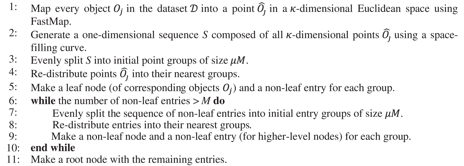
3  FastLoad: Fast Bulk Loading Algorithm

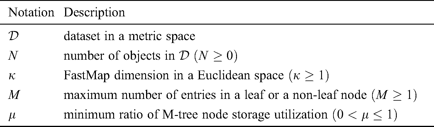
Our first M-tree bulk loading algorithm, which is called FastLoad here, is designed to improve the index construction and search performance by minimizing the number of distance computations and disk accesses. Alg. 1 shows the structure of FastLoad, and Tab. 1 summarizes the notations in this study.

Table 1: Summary of notations

Algorithm 1: FastLoad Algorithm

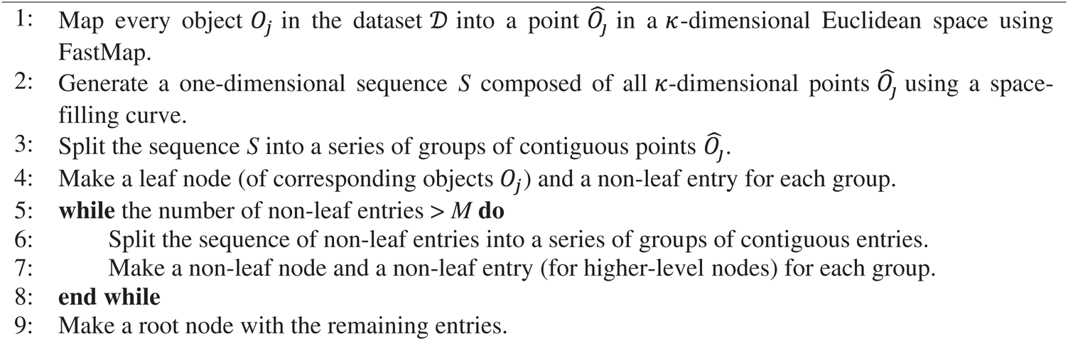
Each step of Alg. 1 is described in detail. In line 1, FastLoad maps each object (j = 1..N) in a dataset in a metric space to a point in a -dimensional Euclidean space using FastMap. With respect to the arbitrary given in advance, FastMap finds the points such that the relative distances are maintained as much as possible [15].

In line 2, the -dimensional points obtained above are sorted to generate a one-dimensional sequence S of the points. FastLoad uses a space-filling curve [16] to have the points that are close to each other in the -dimensional space remain at a minimal distance in the one-dimensional sequence. The space-filling curve sequentially visits each object once on the -dimensional grid, and the order of each point is determined based on the visiting order. Among many space-filling curves including Z curve, Hilbert curve, and Gray-code curve, FastLoad uses the Hilbert curve.

In line 3, the one-dimensional sequence S is partitioned to create a series of groups of contiguous points, where is the minimum storage utilization ratio. In line 4, a leaf node is created for each group with the objects in the metric space corresponding to all points in the group. Since the one-dimensional sequence was generated such that the relative distances of the objects in the original metric space are closely maintained, it is highly probable that the objects corresponding to the points in a group are actually close to each other in the metric space also.

In line 3, the one-dimensional sequence S is partitioned into groups as follows. S is scanned from the beginning and the first contiguous points in S are extracted to form a group G of the points. For the sequence of the remaining points, the same task is performed repetitively until there are or less points in the sequence. To maximize the space utilization of an M-tree, it is best to include M points in every group. However, even for the points and in the same group, their corresponding objects and in the metric space may be distant from each other. In such a case, the size of the node region corresponding to the group will increase, thereby degrading the search performance. In this study, we propose three partition methods, named FULLPAGE, HEURISTIC, and RIGOROUS, as follows:

•   FULLPAGE All groups are fully filled with M contiguous points.

•   HEURISTIC Each group is initially filled with points, and is computed, where d is the distance between the first and the last points in the group, and is the number of points. For each subsequent point extracted from S and added in the group, is computed, where is the distance between the first and the newly added points, and is the number of points. If , it indicates that the average region size for each point increases; therefore, the group is finalized with points.

•   RIGOROUS Among the candidate groups containing contiguous points, the one with the smallest is chosen, where r is the radius of the corresponding region, and n is the number of points.

In the HEURISTIC and RIGOROUS methods, since the actual distance d() between two objects and in the metric space is expensive to compute, it is replaced with () between two points and in the -dimensional Euclidean space. By sacrificing a small degree of correctness, the speed of distance computation is improved.

A leaf node for a point group is generated as follows. While -dimensional points were used for generating groups of contiguous points, the original objects in the metric space are used for M-tree node generation. A leaf node is represented by a circular region centered by with radius . The distance is computed for all object pairs to determine the object that satisfies Eq. (1), and the complexity is as high as . Therefore, in FastLoad, is set to be an object corresponding to the point that minimizes , where is the -dimensional Euclidean center of the region containing all points in the group, and is computed using the actual distance d(), i.e., . The complexity for computing “cheap” distances () to find and is , and that for computing “expensive” distances d() is reduced to . The complexity of distance d() computations for all groups is , assuming that the total number of groups is . Note that M is not changed depending on the application and dataset size N, which is much larger than .

For each leaf node generated in line 4, one non-leaf node entry is generated. In lines 6 and 7, the tasks similar to those in lines 3 and 4 are performed for the sequence of non-leaf entries. When splitting the sequence into a series of groups of contiguous entries in line 6, one of FULLPAGE, HEURISTIC, and RIGOROUS methods is chosen as in line 3. While only the distance between two points in each group is considered in line 3, the radius of the region for each entry is also considered in line 6 as shown in Eq. (2), i.e., = , where and denote any two entries in the group. In line 7, the tasks similar to those in line 4 are performed, except that Eq. (2) is used to determine the parent object. Lines 6 and 7 are executed repeatedly, and when the number of non-leaf entries is less than or equal to M, the entries are stored in the root node.

The overhead of distance computations in FastLoad is as follows. The complexity of FastMap in line 1 of Alg. 1 is [15]. The complexity of HEURISTIC and RIGOUROUS methods in lines 3 and 4 is as explained above ( for FULLPAGE). Therefore, the overall complexity of FastLoad is , which is lower than the complexity of BulkLoad since in most cases.

The complexity presented above is related to the “number” of distance computations. The overall computational complexity should be the product of the number of distance computations and the cost of a single distance computation. In general, applications dealing with objects in metric spaces have various definitions of “expensive” distances d() as mentioned in Section 1, and in most applications, the complexity of computing distance d() is much higher than that of computing “cheap” distance (), which is at most . Therefore, in our study, we contributed in reducing the overall computational overhead by reducing the number of “expensive” distance computations from to when making each node.

The overhead of disk accesses in FastLoad is as follows. In Alg. 1, lines 4, 7, and 9 access the disk, i.e., store the M-tree nodes in the disk. Since the leaf nodes generated in line 4 do not have to be referred to anywhere else, they are stored in the disk sequentially. The same is also true for the non-leaf nodes generated in lines 7 and 9. Therefore, the number of disk accesses in FastLoad is equal to the number of nodes in the final M-tree. In general, sequential access of disk pages (or M-tree nodes) is much faster than random access of the same number of pages. The performance of FastLoad can be improved further by saving the nodes in a memory buffer and later flushing them altogether simultaneously in the disk at an appropriate time point, rather than storing each of them immediately and separately in the disk. In case of sufficient memory size, only a single sequential disk access can store the entire M-tree in the disk, thereby further improving the performance of FastLoad.

The performance of FastLoad can be improved further, by simple parallelization in a multi-core environment, as follows. In lines 1 and 2, the computations of distances in FastMap and space-filling curves can be performed in parallel in multiple concurrent threads as they are independent for each object. In lines 3 and 4, the one-dimensional sequence S is divided into a few sub-sequences of possibly different sizes, and each sub-sequence is assigned to one of concurrent threads to construct the corresponding sub-tree in parallel. In the parallel algorithm by Qiu et al. [11], since the number of objects assigned to each thread is not constant, the objects or sub-trees should be exchanged among threads, which dramatically reduces the degree of parallelization. In contrast, FastLoad is more efficient, since all operations in each thread can be run independently of the others.

4  FlexLoad: Flexible Bulk Loading Algorithm

Our second bulk loading algorithm, which is called FlexLoad here, is designed to improve the search performance further by gathering nearby objects in a node using a partitioning clustering technique [19]. In case the number of objects in a node exceeds the capacity of a disk page, the node is stored in multiple contiguous disk pages. This feature of FlexLoad is an adaptation of the concept of X-tree supernodes [20]. Berchtold et al. [20] found that as the dimension of a Euclidean space increases, the overlap between the node regions in an R-tree storing the points in the space also increases, thereby degrading the search performance heavily. An X-tree supernode is made when it is anticipated to be beneficial to avoid splitting into a few nodes for better search performance. The M-tree built by FastLoad also suffers from a similar phenomenon when dealing with the datasets originating from a high-dimensional Euclidean space or real-world datasets requiring high dimension for FastMap. In general, accessing sequential disk pages is much more efficient than randomly accessing the same number of disk pages, and the cost of accessing a few sequential disk pages is almost equal to that of accessing one disk page. Therefore, FlexLoad is anticipated to have a better search performance; the experimental results will be shown in the next section.

Alg. 2 shows the structure of FlexLoad, which is very similar to that of FastLoad; lines 3 and 6 of Alg. 1 are replaced with lines 3~4 and 7~8 of Alg. 2, respectively. In line 3 of Alg. 2, the point sequence S generated in line 2 is evenly split into a set of point groups of equal size without using any specific splitting method, such as FULLPAGE, HEURISTIC, and RIGOROUS, in FastLoad. In line 4, the points in the groups are re-distributed to gather nearby points and thereby minimize the size of regions of the point groups, as shown in Alg. 3. Lines 7~8 of Alg. 2 perform the same operations for non-leaf entries as lines 3~4.

Algorithm 2: FlexLoad Algorithm

Algorithm 3: Re-distribution of points in FlexLoad

In Alg. 3, the “while” loop continues until there is no change in the point groups or for pre-specified times. In the experiments detailed in the next section, we obtained good groups by repeating the loop only 2~3 times. In each iteration, the -dimensional Euclidean center of the region containing all points of each group is computed as in FastLoad. Then, the closest center is found for each point in all the groups, and the latter is moved into the corresponding group . Here, we use the “cheap” distance () for efficient index construction as in FastLoad.

The groups obtained by Alg. 3 contain a variable number of points depending on the actual object distribution, and some groups may contain more than M points. In such a case, even when the overfull group is split into a few groups of sizes , those groups are very likely to be accessed together during the search owing to the locality of the points in the groups. Moreover, if the split groups are stored in the nodes scattered in the disk and/or the sum of the regions of the split groups is larger than the region of the before-split group, there will be a severe degradation in overall search performance. Therefore, FlexLoad stores the point group of size in a node composed of multiple contiguous disk pages in a manner similar to that by the X-tree [20].

FlexLoad has almost the same cost for distance d() computations and disk accesses as FastLoad. Lines 3~4 and 7~8 in Alg. 3, which are the only portions different from Alg. 1, compute only () distances as explained above. The nodes created by FlexLoad are only stored in the disk and never accessed again as in FastLoad. Lines 3~5 of Alg. 3 incur substantial computational overhead since () distance must be computed for each combination of centers and points and it is repeated a few times in the “while” loop. However, since each distance computation is independent and can be performed concurrently with the others, the overall execution time of FlexLoad can be reduced by simple parallelization; the distance computations in lines 3~5 are distributed in many concurrent threads. Our experimental result revealed that the parallelization improved the performance of FlexLoad by 2.4 times on average. Since FastLoad is parallelized similar to FlexLoad, we believe that the performance of a parallel extension of FastLoad is improved to a similar degree.

The spatial complexity of our algorithms, FastLoad and FlexLoad, is , which is needed for storing all -dimensional points obtained using FastMap, as shown in line 1 of Algs. 1 and 2. In our experiments, the largest number of objects in the synthetic datasets is N = 1 M, and the largest dataset dimension is = = 20. By representing each coordinate value as 8-byte double data type, the main memory of size 1 GB is sufficient for running our algorithms. The size (number of POIs) of the largest real-world dataset in our experiments is approximately N = 1 M, and the size of the entire US road network is approximately N = 22.8 M [13,14]. By setting = 8 and using the same data type for coordinate values, the main memory of size 2 GB is sufficient. Since most recent computers are equipped with main memories of considerably larger sizes, the performance of our algorithms is affected only slightly by the size of the main memory.

If an M-tree node is stored in disk whenever it is created by our algorithms, only the representative values shown in Fig. 2a are preserved in the main memory for each node, and the respective nodes are deallocated. In lines 4 and 8 in Alg. 2, when the points are re-distributed, FlexLoad maintains only the center and radius for each point group. These aspects also reduce the effect of the main memory on the performance of our algorithms.

If each M-tree node is stored separately in disk, it incurs random disk accesses. If all the M-tree nodes are gathered in a main memory buffer and are stored in disk together in the end, it incurs only a single sequential disk access. In general, sequential access on HDDs and SSDs is more efficient than a random access of the same size at the cost of the main memory buffer. The sizes (in MBs) of the M-trees built by using our algorithms are small, as shown in Tabs. 2, 4, and 6; i.e., our algorithms require only a small amount of the main memory even when they gather all the M-tree nodes in a buffer for efficient disk accesses. Therefore, we can see once more that the size of the main memory only slightly affects the performance of our algorithms.

Table 2: Sizes (in MB) of M-trees built by our algorithms for various dataset sizes (N)

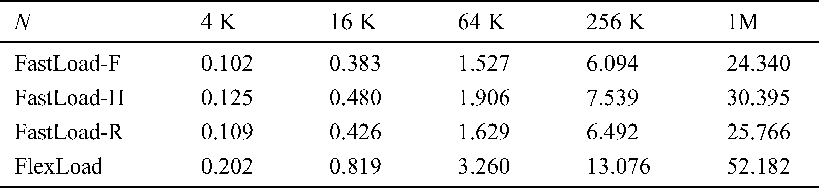
Table 4: Sizes (in MB) of M-trees built by our algorithms for various data dimensions (d)

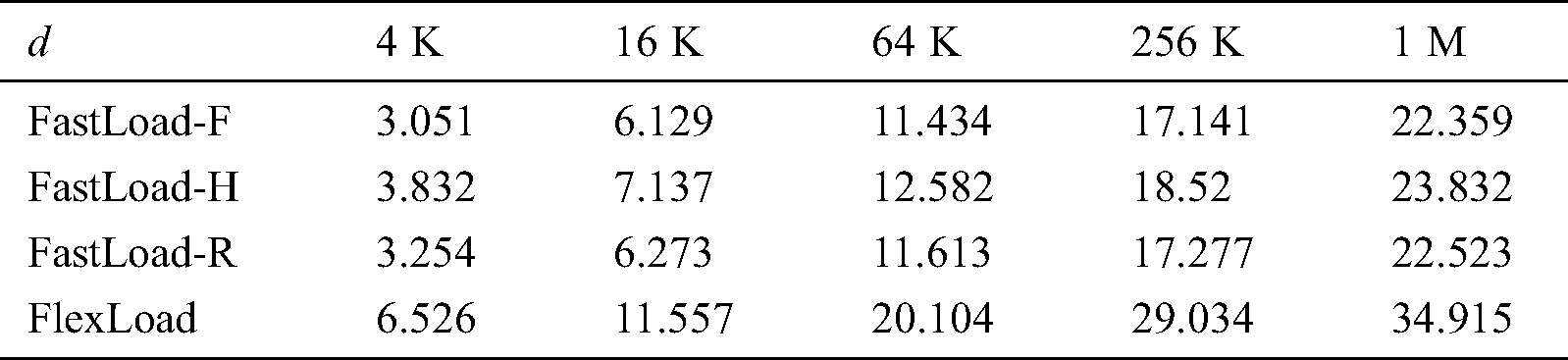
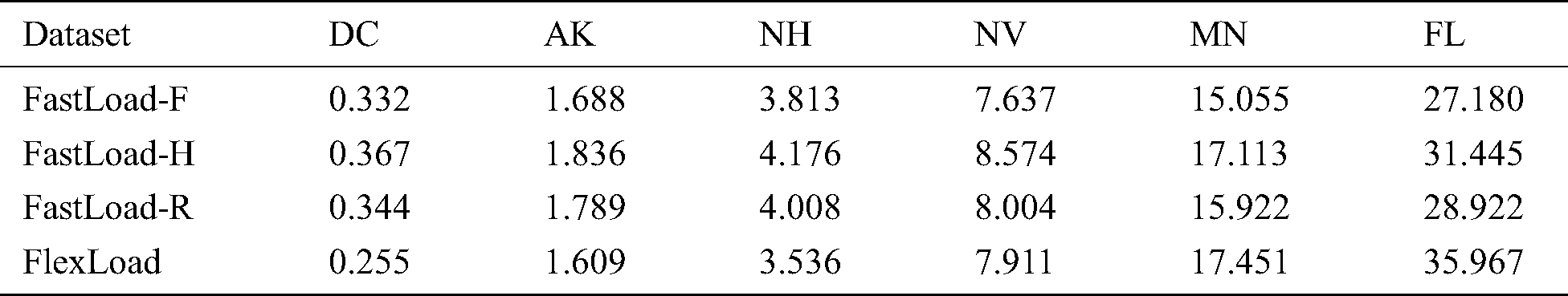
Table 6: Sizes (in MB) of M-trees built by our algorithms for various road networks

5  Experimental Evaluation

In this section, we demonstrate through experiments that our algorithms FastLoad and FlexLoad outperform BulkLoad [10] in M-tree construction and search by reducing the number of distance computations and disk accesses. The platform for the experiments is a workstation with an Intel i7-6950X CPU, 64 GB memory, and 512 GB SSD. The CPU has 10 cores and can run 20 concurrent threads. We implemented FastLoad and FlexLoad in C/C++ and used the source code of BulkLoad written in C/C++ by the original authors1.

We use both synthetic and real-world datasets for experiments in this study. The synthetic datasets used in the first through fourth experiments consist of d-dimensional objects contained in eight Gaussian clusters generated using the ELKI dataset generator2. The centers of the Gaussian clusters were randomly chosen in a d-dimensional cube , such that the distance between any two centers was not less than . The standard deviation for each cluster was chosen randomly in the range . We set “expensive” distance d() as the Euclidean distance ( metric) between two objects for all algorithms FastLoad, FlexLoad, and BulkLoad, whose computational complexity is as low as , where d is data dimension, considered to ensure the same settings as in the previous studies. Although such a low complexity is favorable for BulkLoad, we show that FastLoad and FlexLoad outperform BulkLoad.

The first experiment compares the execution time and the number of distance computations and disk accesses while building the M-trees for various dataset sizes N. FastLoad is tested separately for each of the three methods in Section 3. We use two-dimensional synthetic datasets and set = 2 for FastMap. The minimum storage utilization ratios for FastLoad/FlexLoad and BulkLoad are set as = 0.5 and 0.4, respectively, and their disk page sizes are 4 KB. Fig. 3 shows the result of the first experiment. The FastLoad algorithms using the FULLPAGE, HEURISTIC, and RIGOROUS methods are denoted as FastLoad-F, FastLoad-H, and FastLoad-R, respectively. FlexLoad-P stands for a parallel version of FlexLoad as described in Section 4. Note that the vertical axis of Fig. 3a is represented in the logarithmic scale. Tab. 2 summarizes the sizes of the M-trees built by our algorithms for various N. BulkLoad could not finish building the M-tree for a dataset of size 1M. FastLoad-R performed a larger number of distance computations and required longer execution time than the other FastLoad algorithms as expected. FlexLoad also took a long execution time due to () computations, while it performed almost the same number of d() computations and disk accesses as the other algorithms. Figs. 3a–3c show the superiority of our algorithms; especially, FastLoad-F and FastLoad-H outperformed BulkLoad by up to three orders of magnitude.

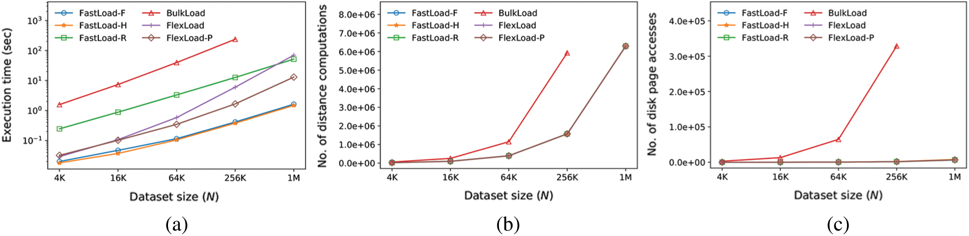
Figure 3: Comparison of M-tree construction performance for various dataset sizes (N). (a) Execution time (seconds). (b) Number of distance computations. (c) Number of disk page accesses

The second experiment compares the k-nearest neighbor (k-NN) search performance for various k values. The dataset of size 256 K used in the first experiment is also used in this experiment. For each k, k-NN search is performed for each of 10,000 random query objects. Fig. 4a shows the average execution time per query in milliseconds. Figs. 4b and 4c show the average number of distance computations and disk accesses. FlexLoad exhibited the best search performance of all algorithms due to gathering manner of nearby objects in the same node described in Section 4. FlexLoad outperformed BulkLoad by up to 20.3 times for k = 1. Among FastLoad algorithms, although FastLoad-R required longer execution time for M-tree construction than the others, its performance for k-NN search was the best. FastLoad-R outperformed BulkLoad by up to 1.85 times for k = 50; FastLoad-F and FastLoad-H also demonstrated similar performances.

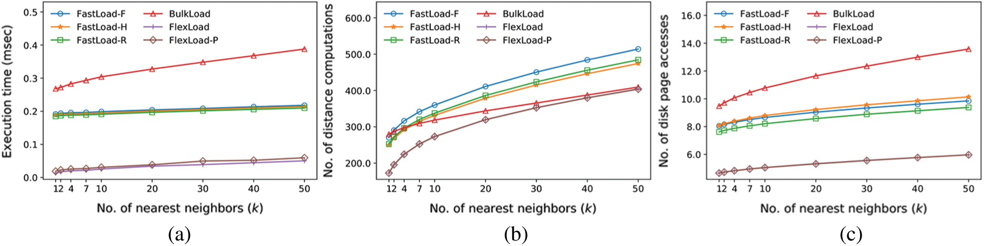
Figure 4: Comparison of k-nearest neighbor search performance using the M-trees (N = 256 K). (a) Execution time (milliseconds). (b) Number of distance computations. (c) Number of disk page accesses

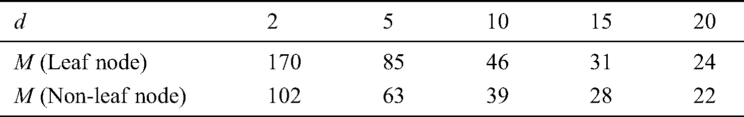
The third experiment compares the M-tree construction performance for various data dimensions d. The dataset of size 128 K in this experiment is generated in the same manner as in the first experiment. We set for FastMap. The value of M for each dimension d in FastLoad/FlexLoad is summarized in Tab. 3. Fig. 5 shows the result. Note that the vertical axis of Fig. 5a is represented in the logarithmic scale. Tab. 4 summarizes the sizes of the M-trees built by our algorithms for various d. In Fig. 5b, as the data dimension increases, the number of distance computations of FastLoad/FlexLoad also increases since for FastMap increases. In Fig. 5c, the number of disk accesses increases since as the data dimension increases the size of an object increases, the number of objects in a disk page of a fixed size decreases, and the number of disk pages to store all objects increases. In Fig. 5a, the execution time of FastLoad-R decreases for since the number of objects in a disk page decreases, and the number of distance () computations to determine for all object pairs in the page also decreases. The execution time of FastLoad-R increases for , owing to the increase in distance d() computations and disk page accesses similar to FastLoad-F and FastLoad-H. Similar to the first experiment, FastLoad-F and FastLoad-H outperformed BulkLoad by up to three orders of magnitude and was faster than even FlexLoad-P. Tab. 3 shows that as d increases, M decreases. With small M values, the performance of an algorithm becomes more sensitive to the cost of an “expensive” distance computation rather than the value of M. Therefore, since FastLoad performs a smaller number of “expensive” distance computations than BulkLoad, we can conclude that FastLoad is superior to BulkLoad.

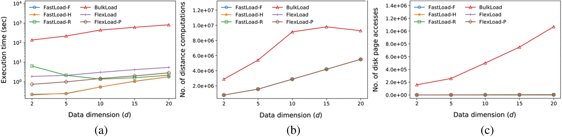
Figure 5: Comparison of M-tree construction performance for various dimensions (d). (a) Execution time (seconds). (b) Number of distance computations. (c) Number of disk page accesses

Table 3: Value of M for each dimension d

The fourth experiment compares k-NN search performance in the same manner as in the second experiment using a 20-dimensional dataset of size 128 K. The result is shown in Fig. 6. FlexLoad again exhibited the best search performance of all algorithms; it outperformed BulkLoad by up to 4.08 times for k = 1. FastLoad algorithms showed worse search performance than BulkLoad. Nevertheless, the difference in searching time for FastLoad and BulkLoad for a single k-NN search is as tiny as about 25 milliseconds. Therefore, FastLoad algorithms are useful in most applications that fast index construction matters and a slight delay in search can be ignored.

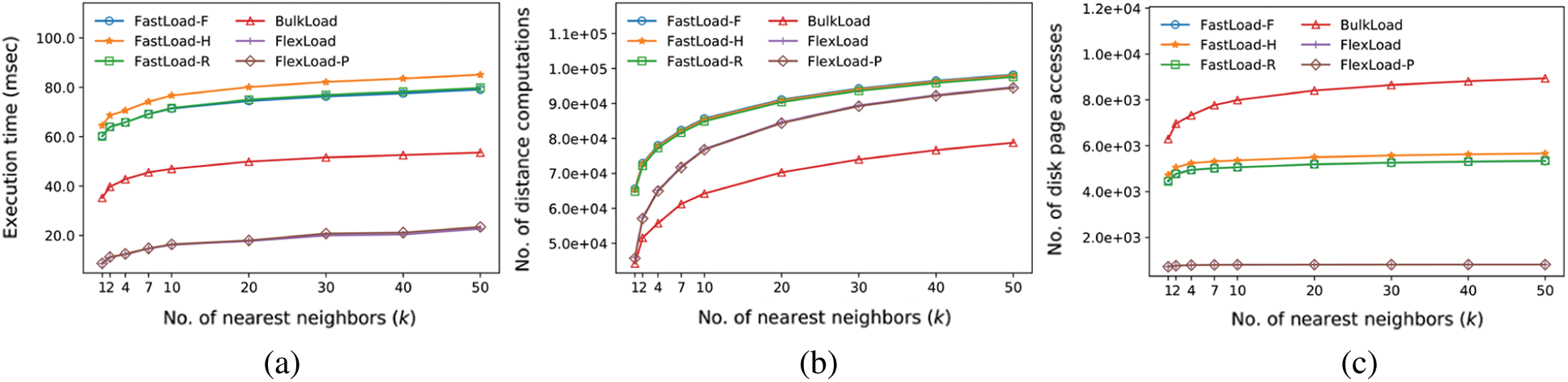
Figure 6: Comparison of k-nearest neighbor search performance using the M-trees (d = 20). (a) Execution time (milliseconds). (b) Number of distance computations. (c) Number of disk page accesses

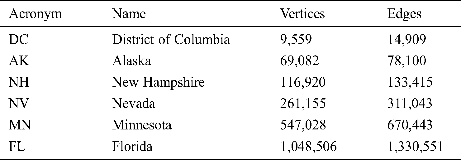
The real-world datasets used in our fifth and sixth experiments are road networks (graphs) from five states and the District of Columbia in the United States, as released by the US Census Bureau and used for the 9th DIMACS Implementation Challenge3 and in many previous studies [13,14]. The datasets are summarized in Tab. 5. Each dataset is composed of a set of vertices (geographic points) and a set of undirected edges (road segments connecting two points). Each vertex consists of its ID and geographical coordinates (longitude and latitude); each edge consists of (source ID, target ID), travel time (weight), spatial distance in meters, and road category (e.g., interstate, local). The datasets include noise such as self-loops and unconnected components as noted in [14]; we cleaned this up in the pre-processing step.

Table 5: Road network datasets

In our experiments, the distance d() between two vertices is defined as their shortest path distance. As explained in Section 1, the complexity to find the shortest path is as high as , where E and V are the number of edges and vertices, respectively. There have been many studies on reducing the computational overhead of the shortest path problem [22–25]. We adopted the pruned highway labeling (PHL) algorithm [26,27], which is known to perform the best at computing the shortest path distance [13,14]. PHL extracts representative shortest paths, such as interstate or highway paths with a small travel time, from the graph; for each vertex, it then stores the distances to the representative shortest paths from the vertex in the index. We used the PHL source code written in C/C++ by the original authors4.

The fifth experiment compares the M-tree construction performance for each of the road network datasets in Tab. 5. We set = 8 for FastMap and the minimum storage utilization ratio as = 0.5 and 0.1 for FastLoad/FlexLoad and BulkLoad, respectively. The results are shown in Fig. 7. Note that the vertical axis of Fig. 7a is represented in the logarithmic scale. Tab. 6 summarizes the sizes of the M-trees built by our algorithms for various road networks. BulkLoad could not finish building an M-tree for the datasets larger than NV, and the higher made it unstable. BulkLoad had a smaller number of distance computations than FastLoad-R and FlexLoad, as shown in Fig. 7b; however, since it made many more disk accesses, as in Fig. 7c, both FastLoad and FlexLoad demonstrated a much better overall performance, as shown in Fig. 7a. FlexLoad needed a longer execution time than FastLoad owing to a number of () distance computations, as in the previous experiments. FastLoad-F and FastLoad-H outperformed BulkLoad by up to three orders of magnitude, as it did in the first and third experiments, and it was also faster than even FlexLoad-P.

Figure 7: Comparison of M-tree construction performance for various real-world road networks. (a) Execution time (seconds). (b) Number of distance computations. (c) Number of disk page accesses

The sixth experiment compares the k-NN search performance using the NV dataset in the same manner as the second and fourth experiments. Fig. 8 shows the result. FlexLoad demonstrated the best performance, outperforming BulkLoad by up to 2.3 times for k = 1. FastLoad algorithms were slightly slower than BulkLoad, as they were in the fourth experiment; however, the difference in execution time for a single k-NN search between the two was only 0.35 milliseconds, which is almost negligible. Therefore, FastLoad is more appropriate than BulkLoad for most applications given its faster index construction.

Figure 8: Comparison of k-nearest neighbor search performance using the M-trees (road network = NV). (a) Execution time (milliseconds). (b) Number of distance computations. (c) Number of disk page accesses

We did not compare the performance of our algorithms, FastLoad and FlexLoad, with that of the algorithms in [11,12] since it is evident that our algorithms significantly outperform them. The objective of the algorithm by Sexton et al. [12] is to improve the search performance using the M-tree, rather than fast construction of the M-tree. As mentioned in Section 2, the complexity of constructing an M-tree using the algorithm [12] is as high as , which is considerably higher than the complexity of BulkLoad [10]. In addition, there is no claim regarding the performance for constructing M-trees in [12]. The algorithm by Qiu et al. [11] simply splits the tasks of BulkLoad among multiple CPU cores, as described in Section 2. Thus, the ratio of the performance improvement cannot be higher than the number of CPU cores, and an experimental result showed that the performance improved by up to 2.33 times when using a quad-core CPU [11]. Since our algorithms outperform BulkLoad by up to three orders of magnitude, it is clear that they also dramatically outperform the algorithms by [12] and [11].

6  Conclusions

In this study, we proposed two efficient M-tree bulk loading algorithms, FastLoad and FlexLoad, which outperform previous algorithms. Our algorithms minimize the numbers of distance computations and disk accesses using FastMap [15] and a space-filling curve [16], thereby significantly improving the index construction and search performance. We experimentally compared the performance of our algorithms with that of a previous algorithm, BulkLoad, using various synthetic and real-world datasets. The results showed that both FastLoad and FlexLoad improved the index construction performance by up to three orders of magnitude and that FlexLoad improved the search performance by up to 20.3 times.

FlexLoad required a longer execution time for index construction than the FastLoad algorithms owing to a number of () distance computations, as described in Section 4, even under similar numbers of distance d() computations and disk accesses. Additionally, FastLoad-F and FastLoad-H were shown to be faster than FlexLoad-P. However, as anticipated, FlexLoad achieved a better search performance than the FastLoad algorithms. Furthermore, although the FastLoad algorithms were slightly slower than BulkLoad for certain datasets, the difference was mostly negligible. In conclusion, we believe that both FastLoad and FlexLoad can be used in a variety of database applications.

Funding Statement: This work was supported by the National Research Foundation of Korea (NRF, www.nrf.re.kr) grant funded by the Korean government (MSIT, www.msit.go.kr) (No. 2018R1A2B6009188) (received by W.-K. Loh).

Conflicts of Interest: The authors declare that they have no conflicts of interest to report regarding the present study.

References

1.   R. Datta, D. Joshi, J. Li and J. Z. Wang. (2008). “Image retrieval: Ideas, influences, and trends of the new age,” ACM Computing Surveys, vol. 40, no. 2, pp. 5–60. [Google Scholar]

2.   B. Kulis and K. Grauman. (2009). “Kernelized locality-sensitive hashing for scalable image search,” in IEEE 12th Int. Conf. on Computer Vision, Kyoto, Japan, pp. 2130–2137.

3.   A. W. M. Smeulders, M. Worring, S. Santini, A. Gupta and R. Jain. (2000). “Content-based image retrieval at the end of the early years,” IEEE Transactions on Pattern Analysis and Machine Intelligence, vol. 22, no. 12, pp. 1349–1380. [Google Scholar]

4.   E. Ioup, K. Shaw, J. Sample and M. Abdelguerfi. (2007). “Efficient AKNN spatial network queries using the M-treeGeographic Information Systems,” in ACM 15th Int. Sym. on Advances in Geographic Information Systems, Seattle, WA, USA, 1–48, 48. [Google Scholar]

5.   K. Shaw, E. Ioup, J. Sample, M. Abdelguerfi and O. Tabone. (2007). “Efficient approximation of spatial network queries using the M-tree with road network embedding Statistical Database Management,” in 19th Int. Conf. on Scientific and Statistical Database Management, Banff, Alberta, Canada: SSDBM, pp. 11. [Google Scholar]

6.   M. L. Yiu, N. Mamoulis and D. Papadias. (2005). “Aggregate nearest neighbor queries in road networks,” IEEE Transactions on Knowledge and Data Engineering, vol. 17, no. 6, pp. 820–833. [Google Scholar]

7.   P. Ciaccia, M. Patella and P. Zezula. (1997). “M-tree: An efficient access method for similarity search in metric spaces,” in 23rd Int. Conf. on Very Large Data Bases, Athens, Greece, pp. 426–435. [Google Scholar]

8.   G. R. Hjaltason and H. Samet. (2003). “Index-driven similarity search in metric spaces,” ACM Transactions Database Systems, vol. 28, no. 4, pp. 517–580. [Google Scholar]

9.   C. Yu, B. C. Ooi, K.-L. Tan and H. V. Jagadish. (2001). “Indexing the distance: An efficient method to KNN processing,” in 27th Int. Conf. on Very Large Data Bases, VLDB, Roma, Italy, pp. 421–430. [Google Scholar]

10. P. Ciaccia and M. Patella. (1998). “Bulk loading the M-tree,” in 9th Australasian Database Conference, Perth, Australia, pp. 5–26. [Google Scholar]

11. C. Qiu, Y. Lu, P. Gao, J. Wang and R. Lv. (2010). “A parallel bulk loading algorithm for M-tree on multi-core CPUs,” in 3rd Int. Joint Conf. on Computational Science and Optimization, Anhui, China, pp. 300–303. [Google Scholar]

12. A. P. Sexton and R. Swinbank. (2004). “Bulk loading the M-tree to enhance query performance,” in 21st British National Conf. on Databases, BNCOD, Edinburgh, UK, pp. 190–202. [Google Scholar]

13. T. Abeywickrama, M. A. Cheema and D. Taniar. (2016). “k-nearest neighbors on road networks: A journey in experimentation and in-memory implementation,” Proc. of the VLDB Endowment, vol. 9, no. 6, pp. 492–503. [Google Scholar]

14. B. Yao, Z. Chen, X. Gao, S. Shang, S. Ma. (2018). et al., “Flexible aggregate nearest neighbor queries in road networks,” in IEEE 34th Int. Conf. on Data Engineering, Paris, France, pp. 761–772. [Google Scholar]

15. C. Faloutsos and K. I. Lin. (1995). “FastMap: A fast algorithm for indexing, data-mining and visualization of traditional and multimedia datasets,” in ACM Int. Conf. on Management of Data, San Jose, CA, USA, pp. 163–174. [Google Scholar]

16. I. Kamel and C. Faloutsos. (1994). “Hilbert R-tree: An improved R-tree using fractals,” in 20th Int. Conf. on Very Large Data Bases, Santiago de Chile, Chile, pp. 500–509. [Google Scholar]

17. I. Borg and P. J. F. Groenen. (2005). Classical Scaling, in Modern Multidimensional Scaling: Theory and Applications. Second. New York, NY, USA: Springer, 261–268. [Google Scholar]

18. V. Silva and J. B. Tenenbaum. (2002). “Global versus local methods in nonlinear dimensionality reduction,” in 15th Int. Conf. on Neural Information Processing Systems, Vancouver, British Columbia, Canada, pp. 721–728. [Google Scholar]

19. J. Han, M. Kamber and J. Pei. (2012). “Cluster analysis: Basic concepts and methods,” in Data Mining: Concepts and Techniques, Third edition, Burlington, MA, USA: Morgan Kaufmann, pp. 443–496. [Google Scholar]

20. S. Berchtold, D. A. Keim and H. P. Kriegel. (1996). “The X-tree: An index structure for high-dimensional data,” in 22nd Int. Conf. on Very Large Data Bases, Bombay, India, pp. 28–39. [Google Scholar]

21. I. Kamel and C. Faloutsos. (1993). “On packing R-trees,” in 2nd Int. Conf. on Information and Knowledge Management, Washington, DC, USA: CIKM, pp. 490–499. [Google Scholar]

22. V. T. Chakaravarthy, F. Checconi, F. Petrini and Y. Sabharwal. (2014). “Scalable single source shortest path algorithms for massively parallel systems,” in IEEE 28th Int. Parallel and Distributed Processing Sym., Phoenix, AZ, USA, pp. 889–901. [Google Scholar]

23. R. Geisberger, P. Sanders, D. Schultes and D. Delling. (2008). “Contraction hierarchies: Faster and simpler hierarchical routing in road networks,” in 7th Int. Workshop on Experimental Algorithms. WEA, Provincetown, MA, USA, pp. 319–333.

24. H.-P. Kriegel, P. Kröger, M. Renz and T. Schmidt. July 2008. , “Hierarchical graph embedding for efficient query processing in very large traffic networks,” in 20th Int. Conf. on Scientific and Statistical Database Management, Hong Kong, China, pp. 150–167.

25. Y. Zhou and J. Zeng. (2015). “Massively parallel a* search on a GPU,” in 29th AAAI Conf. on Artificial Intelligence, Austin, TX, USA, pp. 1248–1254. [Google Scholar]

26. I. Abraham, D. Delling, A. V. Goldberg and R. F. Werneck. (2011). “A hub-based labeling algorithm for shortest paths in road networks,” in 10th Int. Sym. on Experimental Algorithms, Chania, Crete, Greece, pp. 230–241. [Google Scholar]

27. T. Akiba, Y. Iwata, K. Kawarabayashi and Y. Kawata. (2014). “Fast shortest-path distance queries on road networks by pruned highway labeling,” in 16th Workshop on Algorithm Engineering & Experiments, Portland, OR, USA, pp. 147–154. [Google Scholar]

This work is licensed under a Creative Commons Attribution 4.0 International License, which permits unrestricted use, distribution, and reproduction in any medium, provided the original work is properly cited.