Computers, Materials & Continua DOI:10.32604/cmc.2020.012911
Article

A Self-Learning Data-Driven Development of Failure Criteria of Unknown Anisotropic Ductile Materials with Deep Learning Neural Network

Kyungsuk Jang1 and Gun Jin Yun2,*

1Department of Aerospace Engineering, Seoul National University, Seoul, 088262, South Korea
2Institute of Advanced Aerospace Technology, Seoul National University, Seoul, 08826, South Korea
*Corresponding Author: Gun Jin Yun. Email: gunjin.yun@snu.ac.kr
Received: 17 July 2020; Accepted: 27 August 2020

Abstract: This paper first proposes a new self-learning data-driven methodology that can develop the failure criteria of unknown anisotropic ductile materials from the minimal number of experimental tests. Establishing failure criteria of anisotropic ductile materials requires time-consuming tests and manual data evaluation. The proposed method can overcome such practical challenges. The methodology is formalized by combining four ideas: 1) The deep learning neural network (DLNN)-based material constitutive model, 2) Self-learning inverse finite element (SELIFE) simulation, 3) Algorithmic identification of failure points from the self-learned stress-strain curves and 4) Derivation of the failure criteria through symbolic regression of the genetic programming. Stress update and the algorithmic tangent operator were formulated in terms of DLNN parameters for nonlinear finite element analysis. Then, the SELIFE simulation algorithm gradually makes the DLNN model learn highly complex multi-axial stress and strain relationships, being guided by the experimental boundary measurements. Following the failure point identification, a self-learning data-driven failure criteria are eventually developed with the help of a reliable symbolic regression algorithm. The methodology and the self-learning data-driven failure criteria were verified by comparing with a reference failure criteria and simulating with different materials orientations, respectively.

Keywords: Data-driven modeling; deep learning neural networks; genetic programming; anisotropic failure criterion

1  Introduction

Data-driven computational mechanics is one of the branches where the underlying laws such as boundary constraints, material constitutive law, or energy conservation law are replaced or collaborated with the experimental data in non-conventional schemes. Among them, the material constitutive law that has long been based on the traditional empiricism is relatively more influenced by experimental noises/errors or uncertainties than other physics-based law associated with boundary value problems. Owing to advances in measurement science and technologies at multiple scales, traditional empiricism in the material constitutive modeling has started transferring to a data-driven paradigm. Not only does the inundation of data truly make it possible to advance computational mechanics but also the discovery of new physics-based material laws is enabled by emerging applications of data science, material informatics, and artificial intelligence (AI). The true data-driven (i.e., knowledge-based approach) approach was originally proposed by Ghaboussi and his co-workers [1]. They replaced the material constitutive model in the finite element model with an artificial neural network (ANN) form. The resurrection of artificial intelligence through recent deep learning advances has exploded in numerous applications to computational mechanics and material constitutive modeling [2–5]. In particular, Oishi et al. [3] proposed a new method of numerical quadrature enhanced by deep learning for the FEM stiffness matrices. Many researchers have applied ANN to various research fields such as cyclic plasticity [6,7], fiber-reinforced polymeric composites [8–10], rubber materials [11,12], rate-dependent materials [13,14], other composite materials [15,16], finite deformation with hyperelastic material [17] and traction-separation laws by reinforcement learning technique [18]. Recently, Liu et al. [19] also studied a sophisticated 3D network architecture of the deep material network for data-driven multiscale mechanics. Computational discretization by numerical methods such as the finite element method is required to apply ANNs in their problems [4,5].

Beyond the material constitutive modeling, more intrusive approaches of applying deep neural networks in diverse computational physics problems have also been researched recently [20–25]. Based on the idea of solving partial differential equations by ANN [26], Raisssi et al. [20] proposed physics-informed deep learning which models physics laws at random collocation points on the boundary and the domain. This method was improved by an adaptive collocation method for second-order boundary value problems (BVP) [24]. However, the current constraint in AI-based data-driven computational mechanics lies in a scarcity of data. Therefore, there is a pressing need for data-efficient training and modeling approach for solving such mathematically formulated physical problems with the help of deep learning neural networks.

The data-driven approach also encompasses the recent stress-strain data-driven computational mechanics approach originally proposed by Kirchodoerfer et al. [27]. This approach is also a model-free numerical method in the regime of computational mechanics. Their novelty lies in the fact that this approach does not require an explicit form of constitutive equations in their formulation. This approach has been further extended to diverse problems [27–31]. Eggersmann et al. [29] extended Kirchdoerfer and Oritz’s data-driven method to inelasticity. Data from experiment tests have been mainly used for parameter identification [32] or model updating within the empiricism regime rather than replacing those laws or constraints in the boundary value problems. Leygue et al. [33] proposed a methodology called data-driven identification (DDI) that can build materials response data from full-field digital image correlation (DIC) data. They utilized a framework of data-driven computational mechanics (DDCM) by Kirchdoerfer et al. [27]. Stainier et al. [31] combined DDI with DDCM for bypassing the empiricism of material modeling. Further active studies on data-driven mechanics are undergoing by numerous researchers [34–37].

In this paper, we focus more on the aforementioned AI-based data-driven approach where the ANN model entirely replaced material constitutive law in the computational mechanics form [38,39]. ANN material models can predict the nonlinear multi-axial stress-strain relationships both under monotonic and cyclic loading [39]. Intrusive implementation technique of the ANN material constitutive model within finite element analysis codes is available [40,41]. However, one of the challenges with the ANN material constitutive model is the availability of comprehensive stress-strain training data from experiments, which is formidable in usual material tests. For tackling such challenges of ANN models, Ghaboussi et al. [1] proposed an online training methodology called an auto-progressive training whereby ANN material constitutive models are automatically trained in the course of nonlinear finite element analyses subjected to experimental boundary reaction forces and displacements. This powerful method has the advantage of generating sufficient stress-strain training data from global experimental measurements. Symbolic regression technique such as genetic programming is useful for generating mathematical equations from material response extracted by the auto-progressive training algorithm. The online auto-progressive training of ANN models is distinct from straightforward training of ANN models with stress-strain data. On the other hand, the deep learning neural network (DLNN) has a deeper hidden network of the perceptron. The backpropagation training algorithm and conventional activation functions such as hyperbolic tangent or sigmoid functions are not suitable for training the DLNN. Although the DLNN is advantageous in learning massive data, few research on its application to the material constitutive model, nonlinear finite element analysis, and the data-driven modeling have been researched to the best knowledge of authors.

In this paper, we propose a new self-learning data-driven modeling methodology that can discover the failure criteria of uncharacterized materials. Its novelty lies in the first DLNN-based material constitutive model formulated for nonlinear finite element analysis, on-line hybrid numerical/experimental training, data processing, subsequent symbolic regression, and their novel integration. The proposed method is verified through developing a new anisotropic initial failure criterion with a known reference failure criteria and synthetic simulated test data. Significance of the proposed self-learning data-driven modeling idea lies in its new unified and efficient ability to develop failure criteria of new materials such as process-dependent 3D printed materials from minimum experimental test data. This paper is organized as follows. Section 2 explains data-driven finite element analysis with DLNN material constitutive model. Section 3 describes the on-line hybrid numerical/experimental training called the self-learning inverse finite element simulation (SELIFE). It is followed by data processing ideas for identifying failure points and subsequent symbolic regression in Section 4. Section 5 presents a demonstration of the proposed methodology and verification of results with simulated tests. Finally, the conclusions are made in Section 6.

2  Data-Driven Finite Element Analysis with DLNN Material Constitutive Model

The data-driven FE simulation means the nonlinear FE simulations with the DLNN-based material constitutive model, which can be self-organized by experimental measurements. The DLNN version material constitutive model was first attempted in this paper with the derivation of the algorithmic tangent operator to be explained in the following.

2.1 DLNN Material Constitutive Model

Data features for input & output layers and DLNN material constitutive model in the data-driven nonlinear finite element model are shown in Fig. 1. Data features for the input and output layers are defined in terms of stresses and strains. Input features include stress-strain pairs and history-dependent internal variables. The internal variable means the sum of the total energy density at previous increment and incremental strain energy as

Figure 1: A flow of the data-driven FEA with DLNN material constitutive model

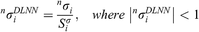
where, and are the stress and strain vector at (n − 1)-th increment, respectively; is the incremental strain, and is the internal variable. Especially, these variables transform one-to-many strain-to-stress mapping to one-to-one mapping between strain and stress values, resulting in a robust learning capability of hysteretic behavior of materials [39]. The sizes of the input and output features depend on the dimensionality of the finite elements. For example, in the case of the plane stress condition, twelve input nodes (i.e., ) and three output nodes (i.e., ) are needed while twenty four input nodes and six output nodes are required in the case of 3D brick linear elements accordingly.

The DLNN model is trained by a supervised learning scheme in the second step of Fig. 1. In particular, stress data from the output nodes are partially fed back into the input nodes of the DLNN recursively since the trained model is used in nonlinear FEA in that mode [39]. Before the training process, stresses and strains should be scaled by each of scale parameters since the stress and strain have different units. Those scaled values should be less than one for effective training.

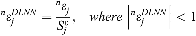
where is the scaled stress value from the DLNN model; is the scaled strain value for the training of the DLNN model; and and are the constant scale values.

Although DLNN can have a deeply hidden network maintaining sufficient learning capability, the formulation in the following assumes two hidden layers. Even if the DLNN can use more than five hidden layers, two hidden layers are sufficient to learn the complexity of the data in this study. Weight factors exist between each of the layers (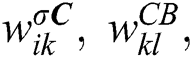 and ). The detailed notations of DLNN parameters are shown in Fig. 2. The Leaky-ReLU function [42] is utilized as an activation function for the DLNN, which is a key to learning with a deep network. Moreover, the adaptive moment estimation (Adam) optimizer [43] was utilized that is specially designed for training DLNN by minimizing the objective function. The objective function is expressed as

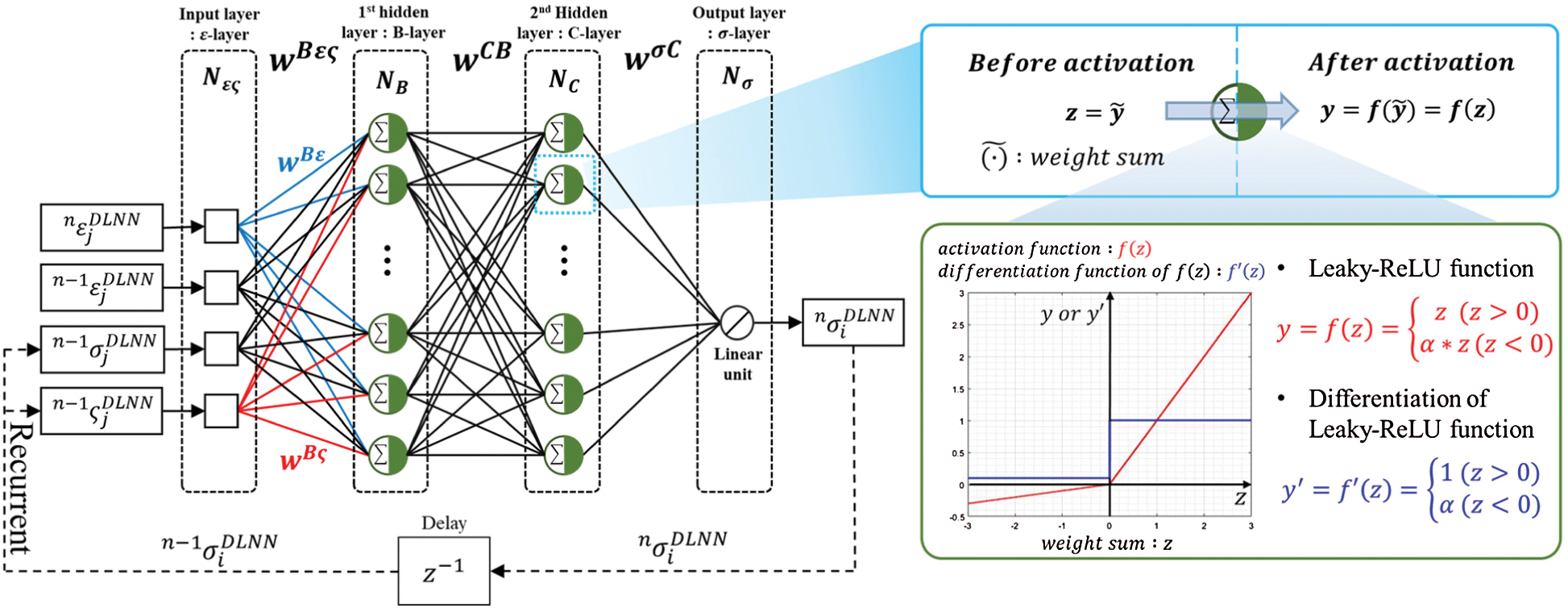
Figure 2: The architecture of DLNN material constitutive model and notations

where is the predicted stress component from DLNN; is the corresponding stress component in the training database; is the index for stress tensor; and is the index for data pattern. The main advantage of the Adam method is that the step size is not affected by the gradient’s rescaling. Besides, the step size can be updated by referring to the past gradient size. Even if the gradient increases, the step size is bound so that stable optimization is possible no matter what objective function is used. From the gradients of the objective function , the Adam optimizer calculates two moment vectors; one is the average of called the 1st-moment vector and the other is the variance of called the 2nd-moment vector . Both moment vectors aids to easily escape out of local minima and to reliably reach a global minimum. However, Adam optimizer is suitable to use in online-training because it requires less effort to tune hyper-parameter (e.g., learning rate ) and save the total simulation time.

The gradient clipping method was applied to prevent the DLNN from exploding in this paper. If the gradient becomes larger during the training, weight parameters are updated with a large gradient and the DLNN model can diverge. It is the exploding gradient problem, which mostly happens in the recurrent neural networks. To deal with this problem, we made the gradient clipped with a limit value . This method is called a gradient clipping [44].

TensorFlow [45,46] was utilized for training the DLNN material constitutive model. The DLNN-based material constitutive model was implemented in ABAQUS UMAT where weight factors of the trained DLNN are accessed through file opening-reading schemes and the Leaky-ReLU activation function is implemented. The trained DLNN will directly predict stresses at the next increment. Finally, the data-driven nonlinear FEA is conducted with the trained DLNN material constitutive model. We call the 3rd step of Fig. 1 as the forward DLNN-based FE simulation.

2.2 Algorithmic Tangent Operator for DLNN Material Constitutive Model

The algorithmic tangent operator (i.e., Jacobian matrix) is required for predicting nonlinear material constitutive behavior. The Jacobian matrix for the DLNN material constitutive model is derived as an explicit function of inputs, outputs and other DLNN parameters such as weight factors ( and ), scale factors ( and ), the derivative form of the activation function and the activation function values from each of the hidden layers in the given DLNN ( and ). The Jacobian matrix can be derived in terms of Leaky-ReLU activation function and other DLNN parameters as follows:

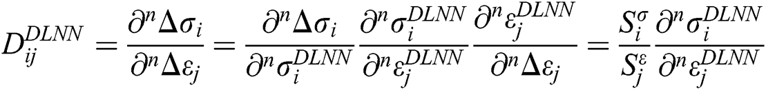
where

and

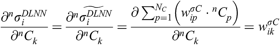
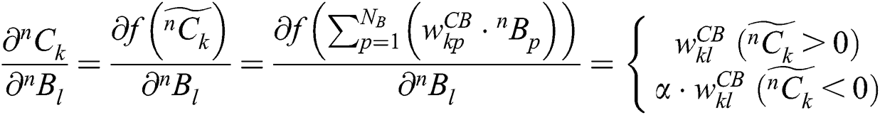
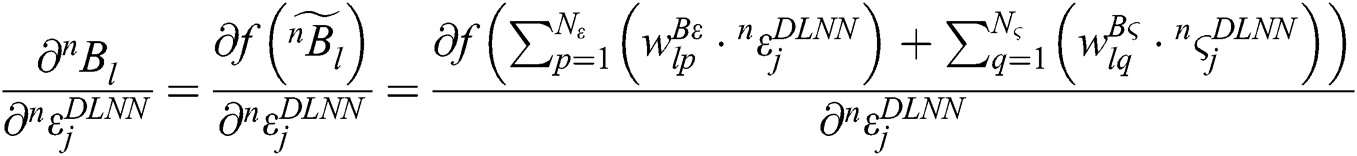
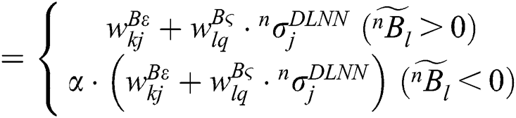
The convergence of this form in the case of multi-degrees of freedom FE models was confirmed as long as the DLNN correctly predicts stress values. The predicted stress and formulated material tangent stiffness matrix are updated at all Gauss points. The global stiffness matrix and external force vector for nonlinear FEA simulation can be updated from stress values and the Jacobian constitutive matrix.

2.3 Comparisons of ANN and DLNN Material Constitutive Models

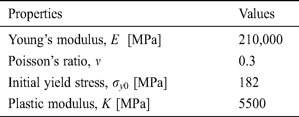
To compare performances of the ANN and DLNN material constitutive models, a reference 2D plane stress FE model subjected to a tensile displacement loading was developed. The plasticity model with linear isotropic hardening was assumed for the reference model. The mesh and boundary conditions are depicted in Fig. 3 and material properties are summarized in Tab. 1.

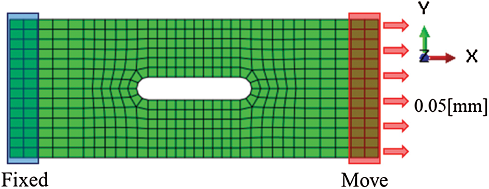
Figure 3: Tensile simulation model

Table 1: Material properties for the reference FE model

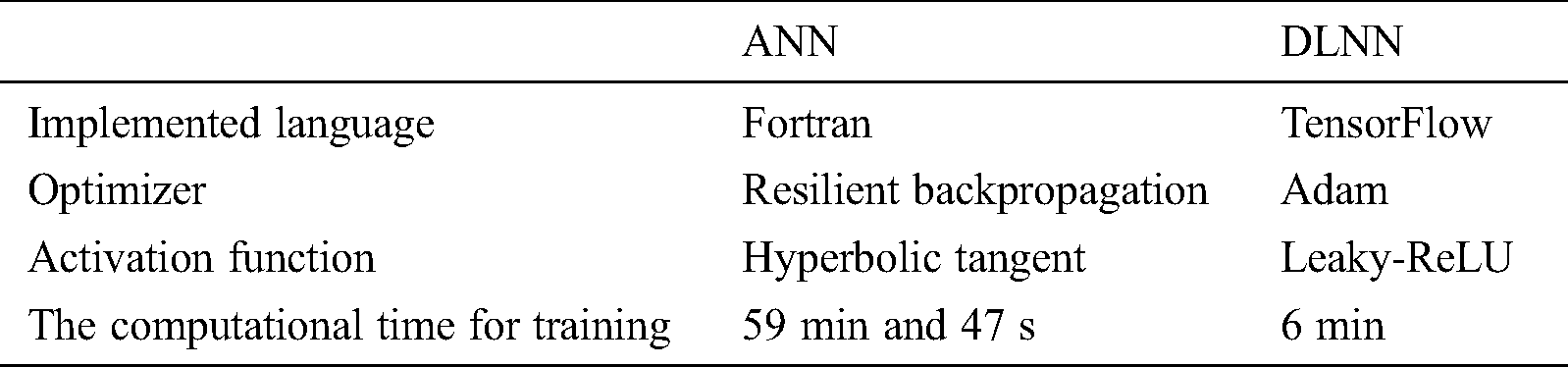
From the reference simulation, stress and strain data were extracted from the whole gauss points within the FE model except for the right and left edges. The total number of training data was 15,040. Neural network structures were set to [12-20-20-3] for both ANN and DLNN models and they were trained until 50,000 epochs. The noticeable differences between ANN and DLNN models are summarized in Tab. 2.

Table 2: Different features between ANN and DLNN

The convergence of the cost function was compared for the ANN and DLNN models as shown in Fig. 4. The convergence of ANN was faster than DLNN until 10,000 epochs. However, the cost value convergence rate of DLNN outperformed ANN after 10,000 epoch, resulting in a much smaller cost value for DLNN than ANN.

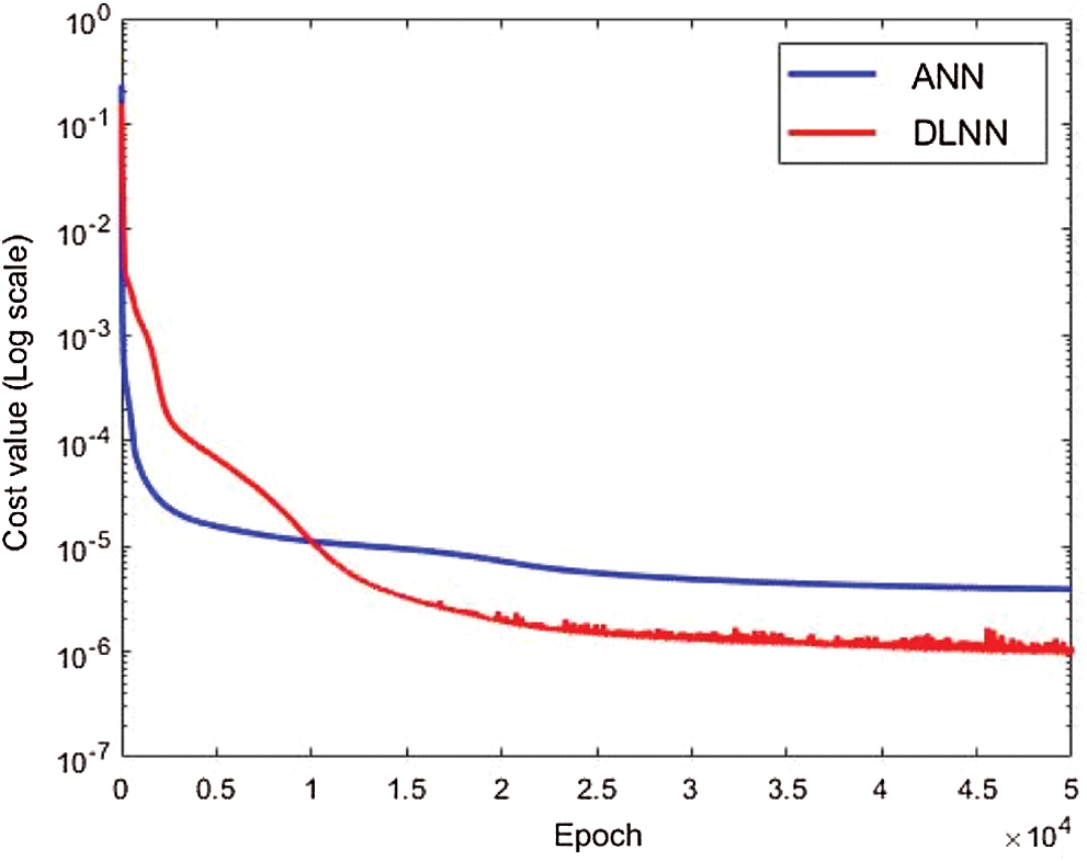
Figure 4: Comparison of variations of cost functions for ANN and DLNN during training

Trained weight factors from the ANN and DLNN model at 50,000 epoch were used in the data-driven FEA. The global force-displacement responses were compared in Fig. 5 and the local responses were compared by enumerating von Mises stress contours as shown in Fig. 6. As expected, the DLNN-based FEA results were closer to the reference FEA results than ANN-based FEA.

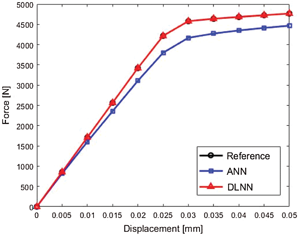
Figure 5: Comparison of global responses (force-displacement) at the right edge

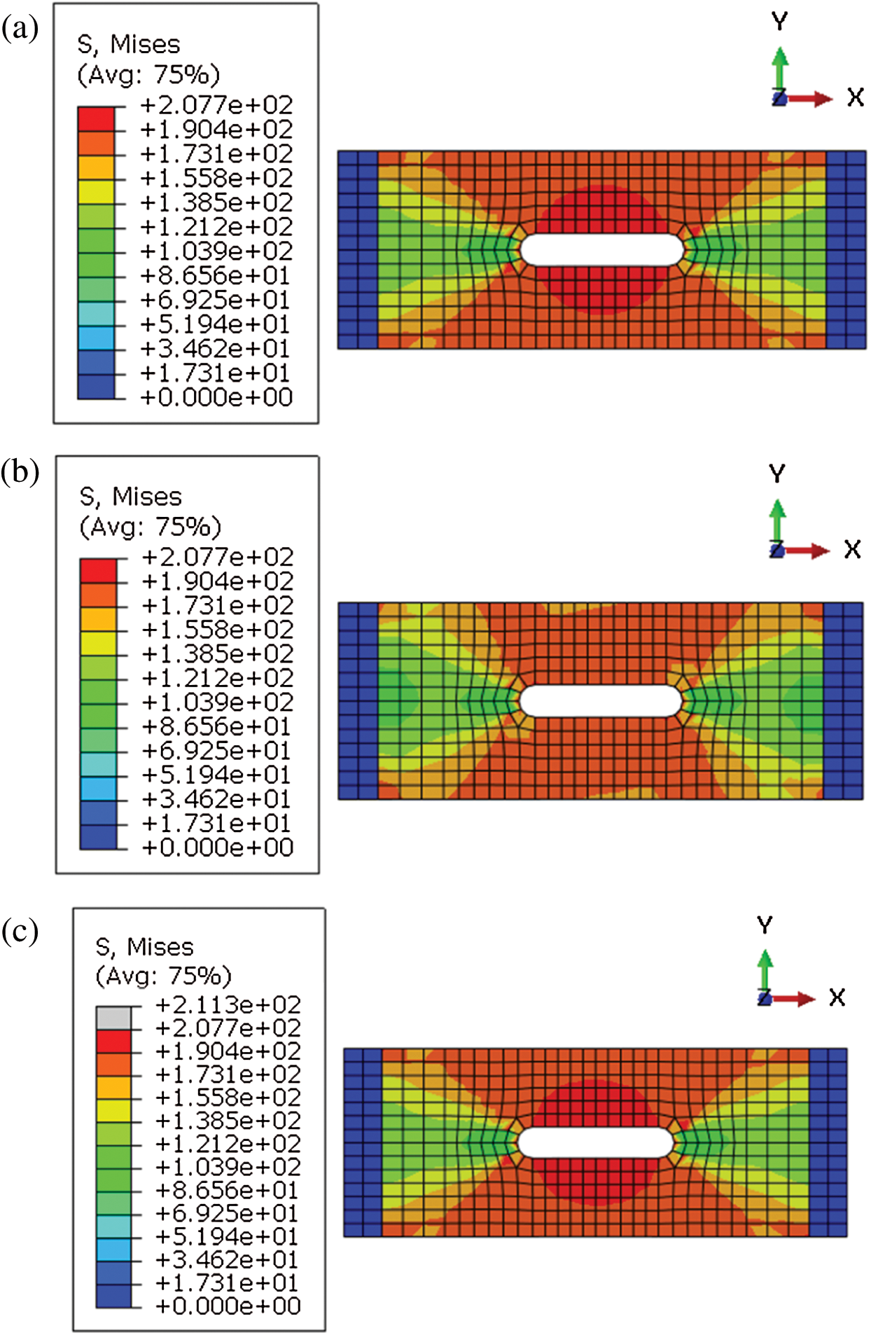
Figure 6: Comparison of von Mises stress contours. (a) Reference FE model with material properties of Tab. 1. (b) ANN-based FEA results and (c) DLNN-based FEA results

For quantitative comparisons, the coefficient of determination (R2) and root mean square (RMS) values were calculated by using the predicted stresses and strains from all FE integration points. They are defined as

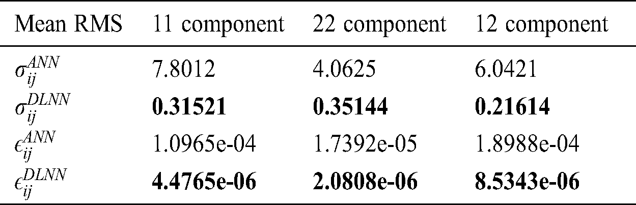
where n is the total number of data; is the true value in the training database; is the mean of , and is the predicted value from DLNN. The averaged R2 and averaged RMS values for each stress and strain component were calculated and summarized in Tabs. 3 and 4, respectively. Overall DLNN performance was better than ANN’s. The mean R2 values for DLNN are closed to one and much higher than the ones for ANN. Moreover, the mean RMS values of DLNN are relatively lower than the ones of ANN. According to the comparative analysis results, we conclude that DLNN is more suitable for material constitutive models than ANN in terms of training speed and accuracy of predictions.

Table 3: Comparison of mean R2 values for each component

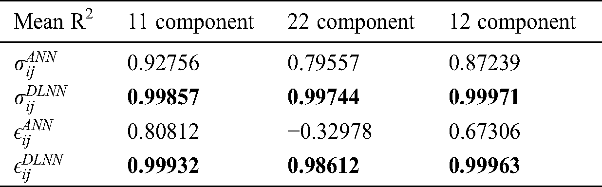
Table 4: Comparison of mean RMS values for each component

3  Self-Learning Inverse Finite Element (SELIFE) Analysis

The SELIFE can obtain complex 3D internal stress-strain states from a set of limited global reaction forces and displacements measured from material and structural tests. Applying inner surface deformation fields from the digital image correlation (DIC) sensor could be advantageous in identifying the 3D complex nonlinear stress-strain paths. Details of the methodology are described in the following.

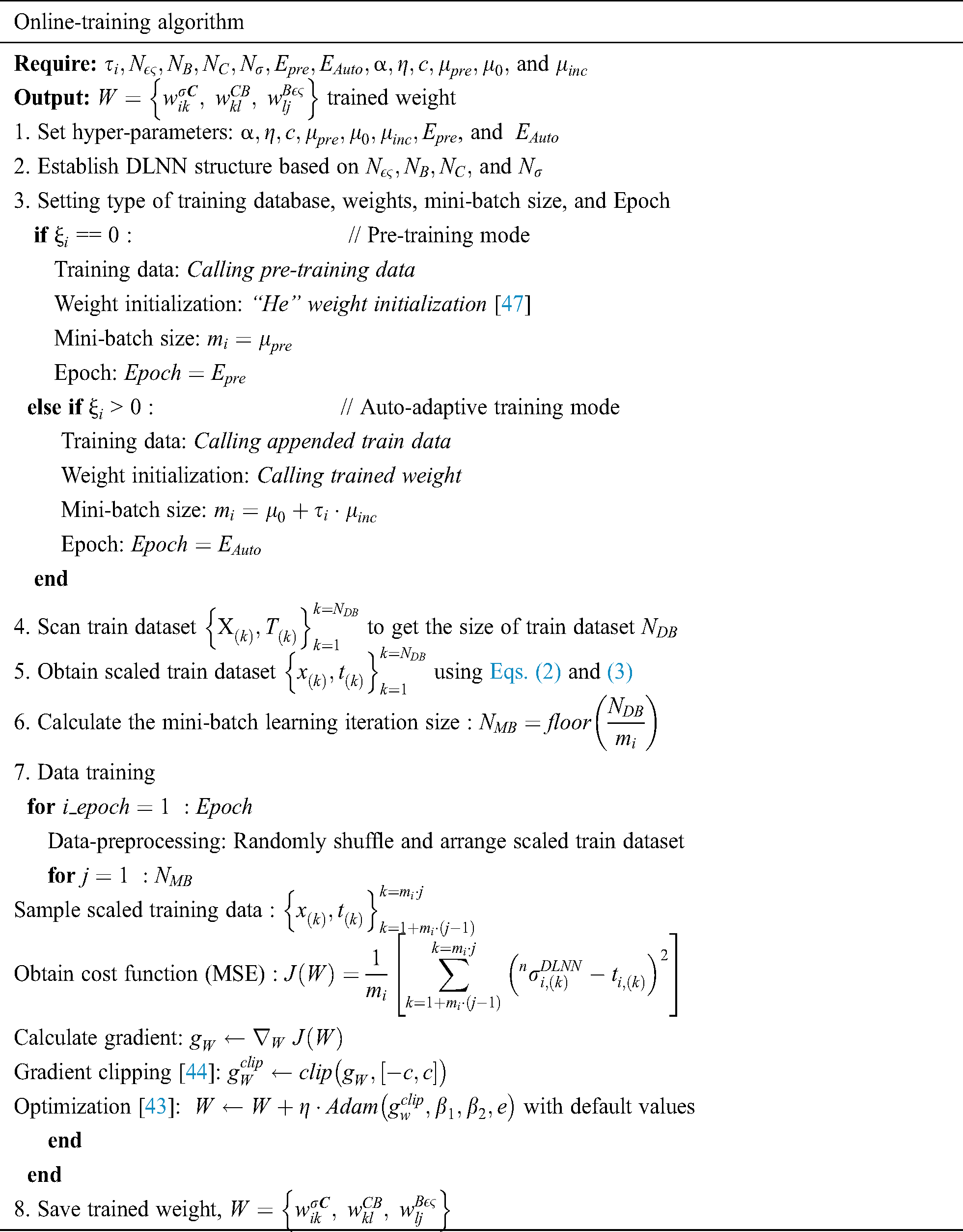
The SELIFE simulation algorithm consists of repeatedly executing the forward DLNN-based FE simulations within an additional auto-adaptive training algorithm at each load (or time) increment. The SELIFE requires two additional iteration loops, which are DLNN pass, and DLNN auto-adaptive training cycle. Sweeping all load (or time) increments is called one DLNN Pass. Multiple DLNN passes may be necessary since the DLNN-based material model may not be trained with only one DLNN pass. In each of the load incremental steps, the SELIFE runs two independent forward DLNN-based FEA, which are the force-controlled analysis (FEM-A) and displacement-controlled analysis (FEM-B) performed within the auto-adaptive training cycles. The stresses and strains at the specified Gauss points from FEM-A and FEM-B, respectively, are appended to the training database. Stresses from FEM-A and strains from FEM-B are better for training the DLNN material constitutive model. Multiple auto-adaptive training cycles are performed until the predetermined number is reached or a convergence criterion in Eq. (11) is satisfied. The criterion is given as:

where is the boundary displacement computed from FEM-A; is the boundary displacement imposed to FEM-B; and is the user-defined tolerance for auto-adaptive cycles. Thus, the criterion is checked as the criteria in each of the auto-adaptive training cycles. The DLNN model is gradually self-organized by the updated training dataset. Computational pseudo-codes, which include the two additional unique iteration loops for the SELIFE, are summarized in Tab. 7.

Table 7: Pseudo codes for SELIFE simulation

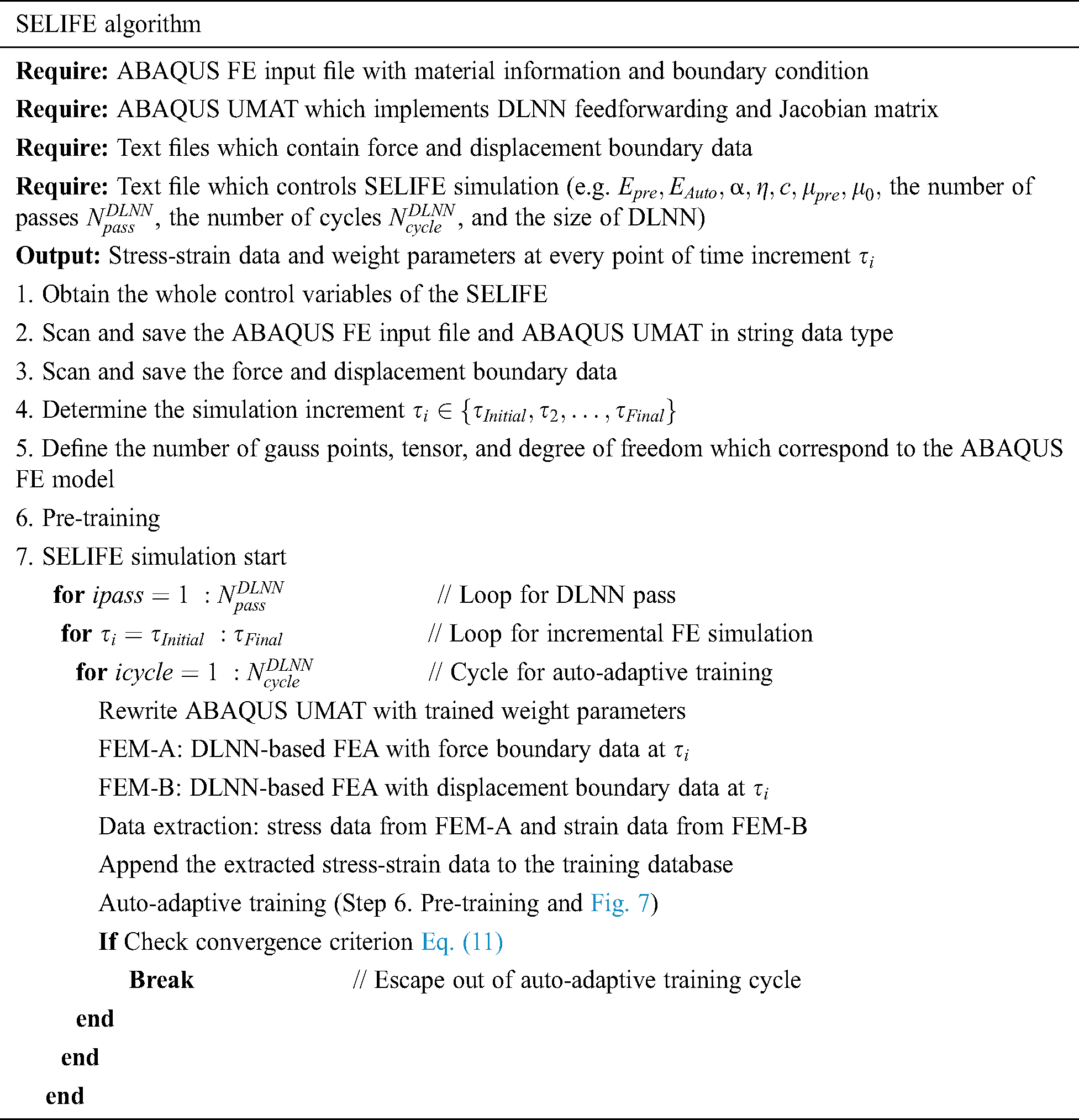
In Fig. 7, the iter1 and iter2 indicate gradual training of the DLNN model toward true stress-strain response through the auto-adaptive training cycles. After the SELIFE simulation, the DLNN model can be used in the forward DLNN-based nonlinear FE analysis. The SELIFE simulation is used to generate material “Big Data” in terms of stress-strain history data, which are subsequently used for establishing the failure criteria of new materials. All notations are summarized in Tab. 5. The pseudo-codes of the online-training in the SELIFE simulation are illustrated in Tab. 6.

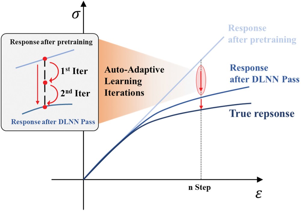
Figure 7: Auto-adaptive learning of true material response

Table 5: Notations and definitions

Table 6: Pseudo-codes for DLNN in the SELIFE simulation

4  Development of Failure Criteria from Self-Learning Data for Unknown Ductile Anisotropic Materials

4.1 Identification Algorithm of Failure Initiation

To develop failure criteria, the initial yield or failure stress data need to be identified based on the obtained multiaxial stress-strain paths from SELIFE analyses. We devised an identification algorithm that accurately pinpoint the failure initiation distinguishing different failure modes. The identification algorithm monitors the tangent stiffness along stress-strain curves. The algorithm for identifying failure initiation consists of two steps. The first step divides the whole multiaxial material response from the SELIFE into nonlinear and linear response paths. The second step of the algorithm determines the stress response point corresponding to the initiation of failure within the whole range of the stress history.

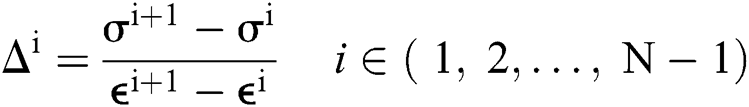
The computational procedures of the first step are shown in Fig. 8a. At the beginning of the first step, stress and strain data are interpolated with a specific number of data points to reduce the effect of noise and error caused by trained DLNN on the calculation of tangent stiffness. It is named as the interpolated tangent stiffness expressed in Eq. (12).

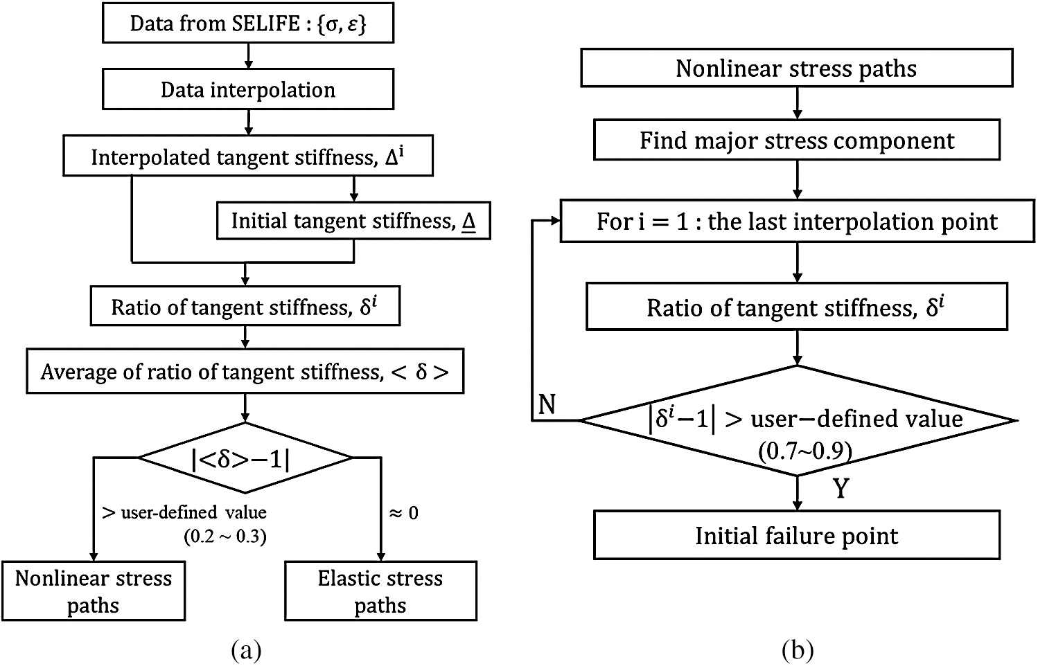
Figure 8: (a) Flowchart for the first step for stress history classification. (b) Flowchart for the second step of the identification algorithm

where indicates the number of interpolations. 50,000 data points were used to interpolate the stress-strain response in this paper. Then, the initial tangent stiffness was evaluated by using the interpolated tangent stiffness within the first two percent of the whole interpolation intervals as follows.

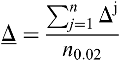
where describes the number of the first two percent interpolation interval.

Then the ratio of the interpolated tangent stiffness to the initial tangent stiffness () is evaluated in Eq. (14). It is followed by computation of the averaged ratio as in Eq. (15). The averaged ratio of the tangent stiffness can classify the stress-strain path into nonlinear and linear regions. According to our experience, the averaged ratio of the tangent stiffness is close to one in the linear elastic range because the tangent stiffness in Eqs. (12) and (13). becomes close to each other within the linear elastic region. However, the averaged ratio of the tangent stiffness deviates from one with the nonlinear stress response regions because the interpolated tangent stiffness values in Eq. (12) become different from the initial tangent stiffness value in Eq. (13). Following this process, we still need an additional step to identify the initial failure point.

In the second step, initial failure points are identified from the nonlinear stress path. In the case of multiaxial stress state, the initial failure point corresponds to the point where the dominant stress component reaches the point earlier than other components Unlike the first step, was used to capture the first deviating point from the initial tangent stiffness. According to our tests, the tolerance value in the range of 0.7~0.9 to be compared with was appropriate to find the initial failure stresses. More detailed procedures for the second step of the proposed algorithm is depicted in Fig. 8b. Once the failure point is determined that corresponds to a specific stress component, then other stress components corresponding to the point are saved for subsequent development of failure criteria.

4.2 Symbolic Regression by Genetic Programming

Genetic programming (GP) is one of the machine learning variants, which is based on a bio-inspired technique. It can derive symbolic equations relating input data with output data out of a training database. It randomly produces tree architectures (e.g., a population consisting of individuals) and operates genetic mutation and cross-over process over the population. Throughout generations, the population converges to the best individual that gives the best performance. Then, the GP can provide a nonlinear equation by assembling weighted linear combinations from the final GP tree structure. An example of the GP tree model is shown in Fig. 9.

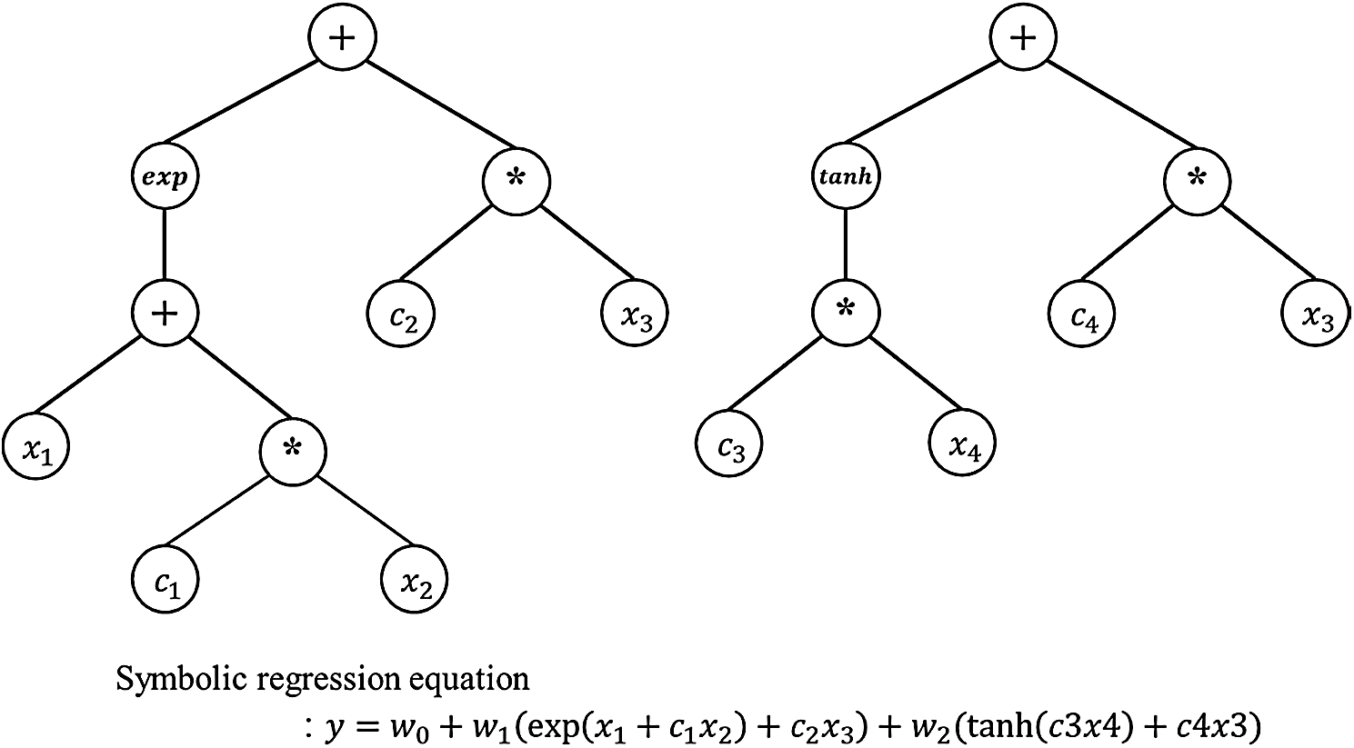
Figure 9: An example of the symbolic regression model by multigene

We utilized one of the genetic programming, called GPTIPS [48], implemented in MATLAB language, and generated an anisotropic yield surface out of the identified dataset. For the effective training of the GP, the data should be prepared. A more detailed process is described in the next section with an example simulation.

5  Verification of the SELIFE and Self-Learning Data-Driven Failure Criterion

For the demonstration of the proposed methodology, we developed a reference biaxial FE model with Hill’s 48 anisotropic failure criterion, which is a reference solution but unknown in actual application to new materials. Therefore, Hill’s 48 anisotropic failure criterion will be compared to the data-driven anisotropic failure criterion. Boundary force-displacement data from the reference simulated tests are deemed to be measurements from experimental tests. A large volume of multiaxial stress-strain data was self-learned and the identification algorithm was applied to discover initial yield stress points. Then, data-driven failure criteria were established by the GP. Finally, the data-driven failure criteria were verified by conducting simulations with different material orientations.

5.1 Simulated Reference Tests with Hill’s Anisotropic Failure Criterion

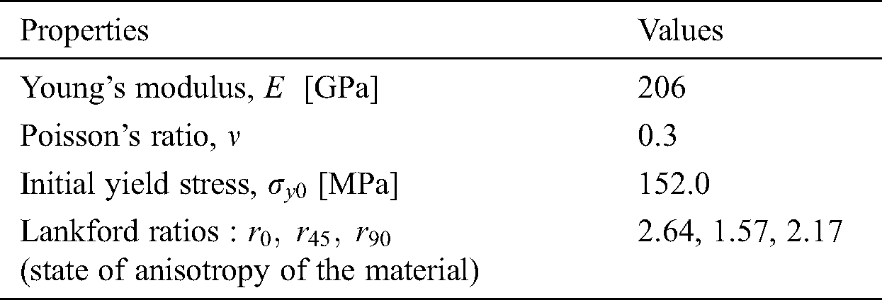
The reference simulated test model is assumed to have anisotropic material with zero degree material orientation and subjected to four-types of displacement boundary conditions (DBC) summarized in Tab. 8. The specimen model is divide into five specific regions as shown in Fig. 10. Displacement of 0.01 mm magnitude was applied in Region A and B while Region C and D were fixed. The DBCs are summarized in Tab. 8. Stress-strain data were extracted from the Region E, where has 256 elements. The 2D plane stress condition was assumed and then the four-node bilinear plane stress (CPS4) element was utilized. Material properties for the simulation are summarized in Tab. 9.

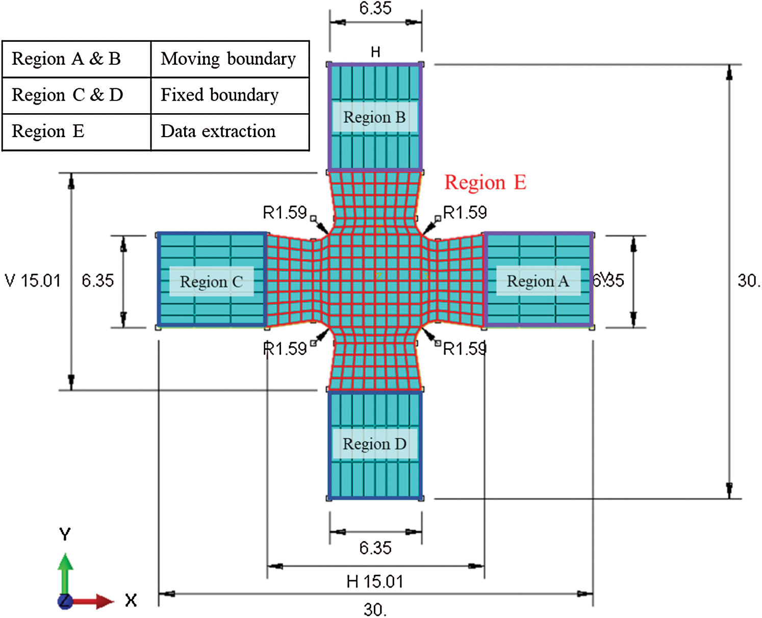
Figure 10: The biaxial specimen with boundary conditions and detail dimension in [mm] scale for the reference simulation

Table 8: Four types of displacement boundary conditions

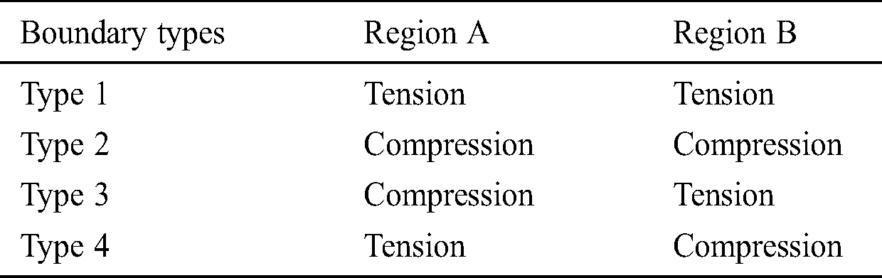
Table 9: Material properties of the anisotropic metal (DDQ mild steel [49])

Hill’s 48 anisotropic failure criterion [50] is defined as follows:

where are the stress components and and are constant parameters that express the current state of anisotropic behavior. The constant parameters are defined as functions of yield stress ratios , the measured yields stress , and the material initial yield stress .

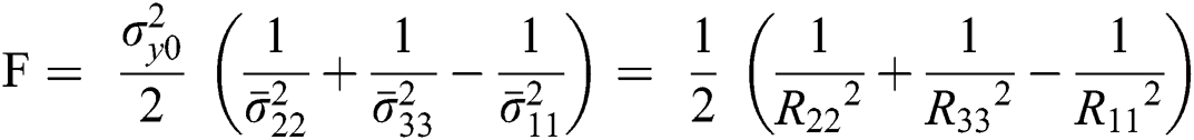
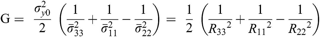
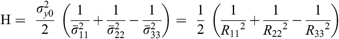
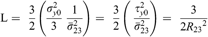
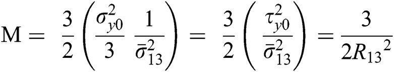
The yield stress ratios are defined as

(for =12, 13, and 23) where

For the plane stress condition, it is convenient to assume as follows [51,52].

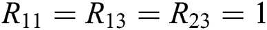
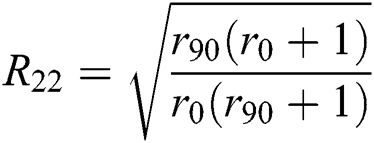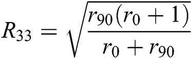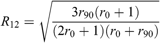, , where and are the Lankford ratios. Moreover, the yield function is reduced to the plane stress condition as follows.

When plastic deformation occurs, the yield function satisfies Eq. (21).

Applying Lankford values in Tab. 9, in Eq. (18) are obtained. Eq. (21) provides the elliptic shape for anisotropic yield surface in the stress space ( and, . The intersections between the yield surface and each of axes define the measured yield stresses. They will be used for the verification of the new data-driven anisotropic yield surface. Applying the uniaxial tensile condition and the pure shear stress condition to Eq. (21), the measured yield stresses () can be obtained. Both yield stress ratios and measured yield stresses are summarized in Tab. 10. The intersection points between the yield surface and axes were numerically calculated that are as shown in Fig. 11. Their values were identical to the measured yield stresses.

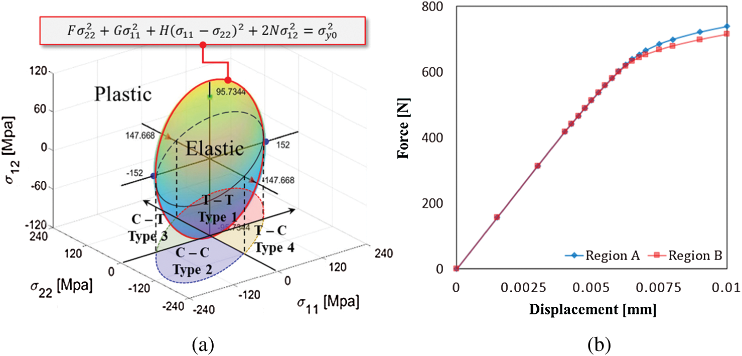
Figure 11: (a) Hill’s 48 anisotropic yield surface with intersections and (b) force-displacement curves from Hill’s anisotropic failure criterion

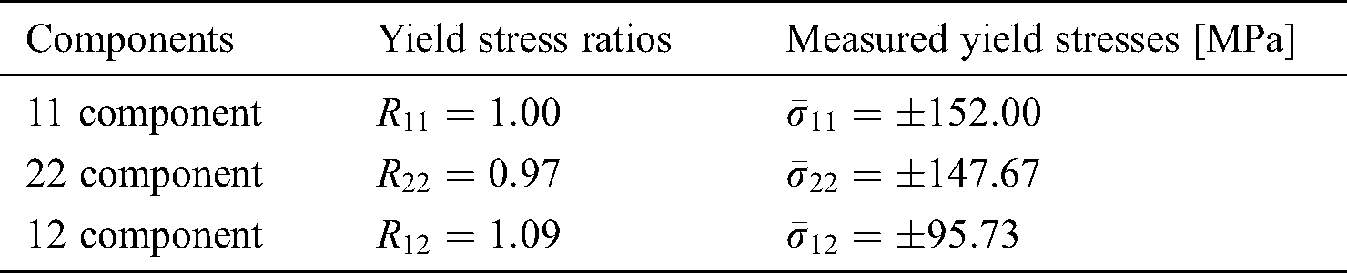
Table 10: Calculated yield stress ratios and measured yield stress

To confirm the anisotropic yield response, the reference simulation with boundary type 1 was investigated. The resultant force-displacement curves measured in Region A and B are different as shown in Fig. 11b.

5.2 SELIFE Simulation Results

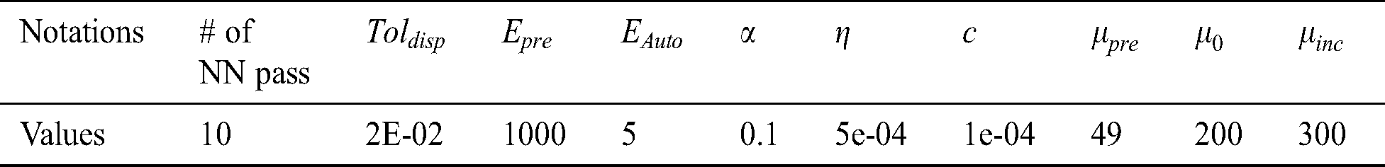
SELIFE simulations were performed with all four boundary types separately. Fifteen nodes in each hidden layer of the DLNN were placed. The DLNN architecture in Eq (22) was used for all SELIFE simulations. Online training was conducted with the same hyper-parameters for DLNN regardless of boundary types. All values for the SELIFE simulations are summarized in Tab. 11.

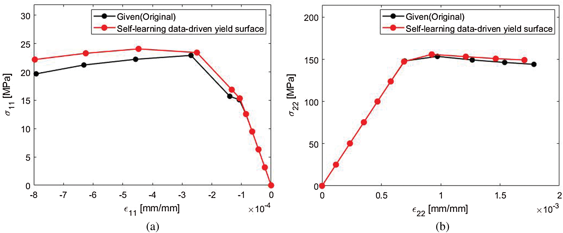
Figure 22: Comparison of stress-strain curves at the 3rd gauss point in the 186th element. (a) 11 component. (b) 22 component

Table 11: Empirically set hyper-parameters for DLNN and parameters of the SELIFE simulation

Effective plastic strain contour under tension-tension DBC (the boundary type 1) at the last analysis step is shown in Fig. 12. To show the local stress-strain path evolution from the SELIFE analysis, two elements were picked: 138th and 132nd elements representing elastic and plastic behavior, respectively.

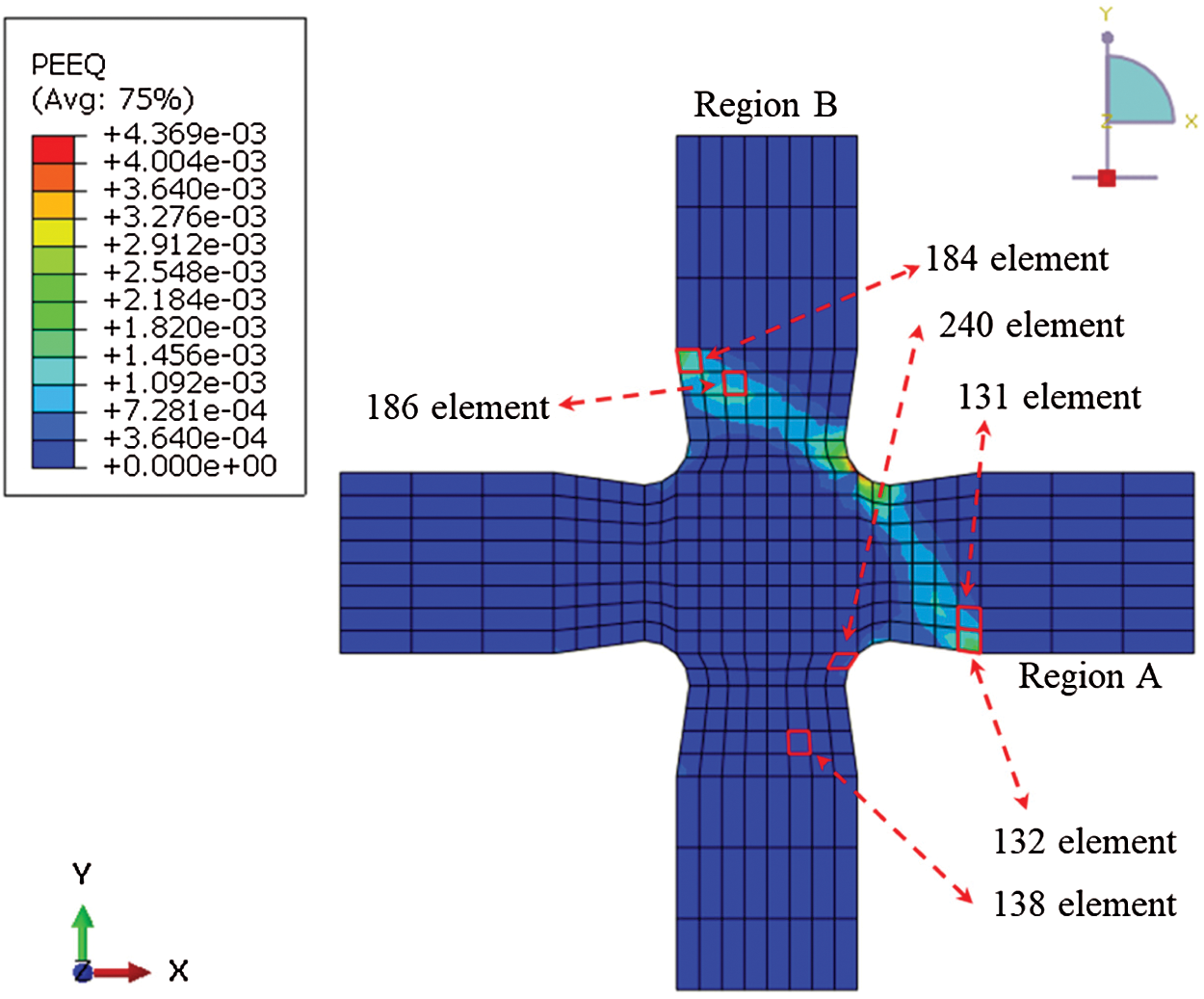
Figure 12: Effective plastic strain contour from the reference simulation under tension-tension displacement boundary condition (boundary type 1)

Fig. 13 shows evidence of the gradual SELIFE learning of global responses. The global reaction force-displacement curve in x-direction, the global reaction force history in the y-direction, and reaction moment history from Region A are depicted in Figs. 13a, 13c, and 13e, respectively. Because of the material anisotropy and the effects of deformation in the other direction, the reaction moment was developed. The global reaction force history in the x-direction, the global reaction force-displacement in the y-direction, and reaction moment history from Region B are illustrated in Figs. 13b, 13d, and 13f, respectively. As evidenced, the global responses gradually approach their targeted curves as the SELIFE DLNN pass increases.

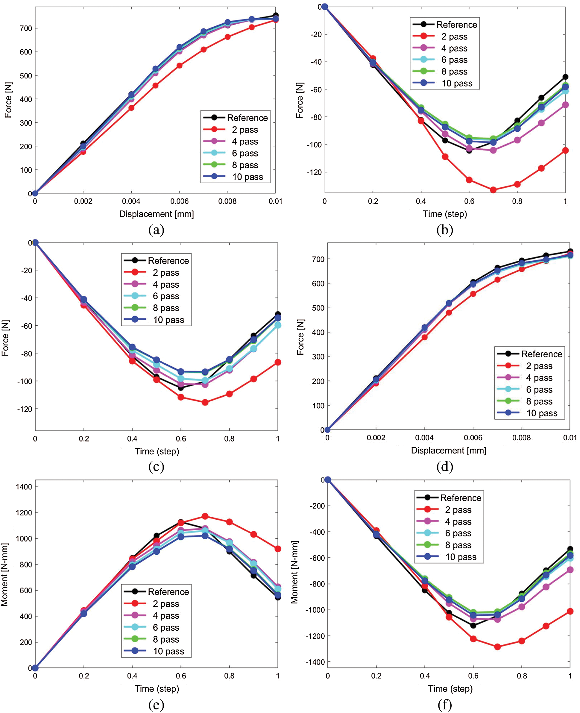
Figure 13: Learning progression of global responses by SELIFE DLNN training; SELIFE simulation under tension-tension displacement boundary condition (boundary type 1). (a) Region A: F-D (x-direction). (b) Region B: F-time (x-direction). (c) Region A: F-time (y-direction). (d) Region B: F-D (y-direction). (e) Region A: F-time (moment). (f) Region B: F-time (moment)

Figs. 14–16 compare local stresses trained by SELIFE with the results from the reference simulation. These results indicate that SELIFE is capable of learning true (i.e., reference) stress-strain relationships.

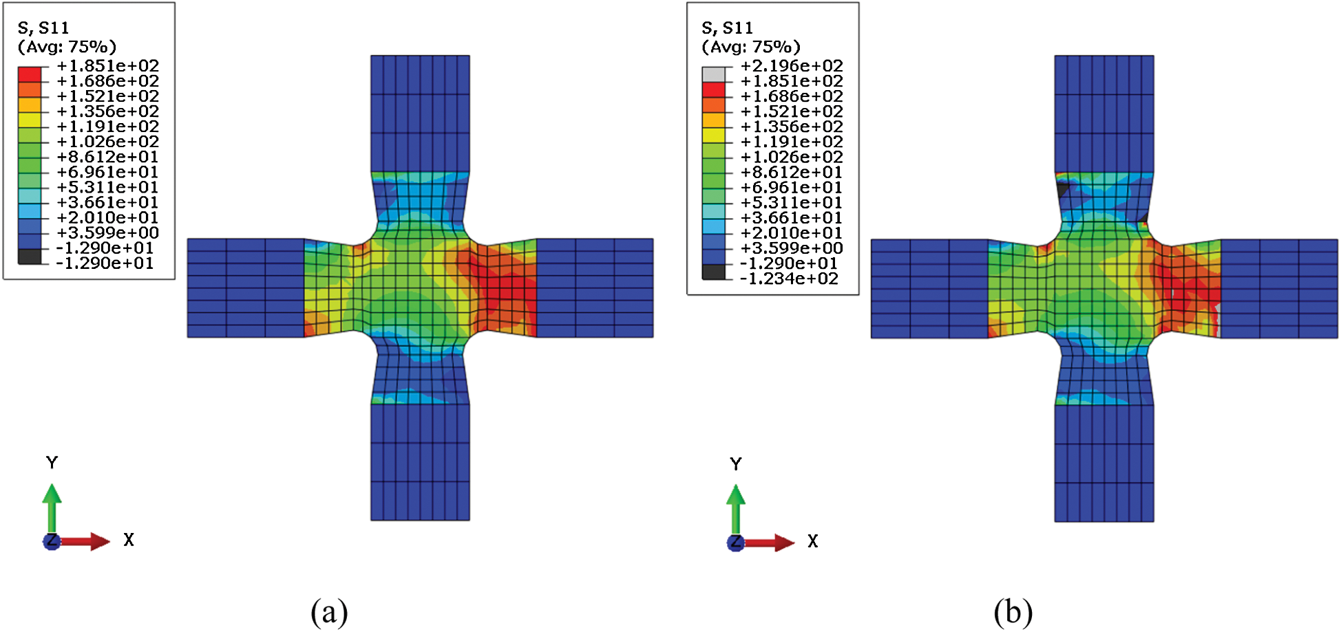
Figure 14: Stress (S11) contour comparison. (a) Result of the reference simulation and (b) result of SELIFE simulation at the last pass (the 10th pass)

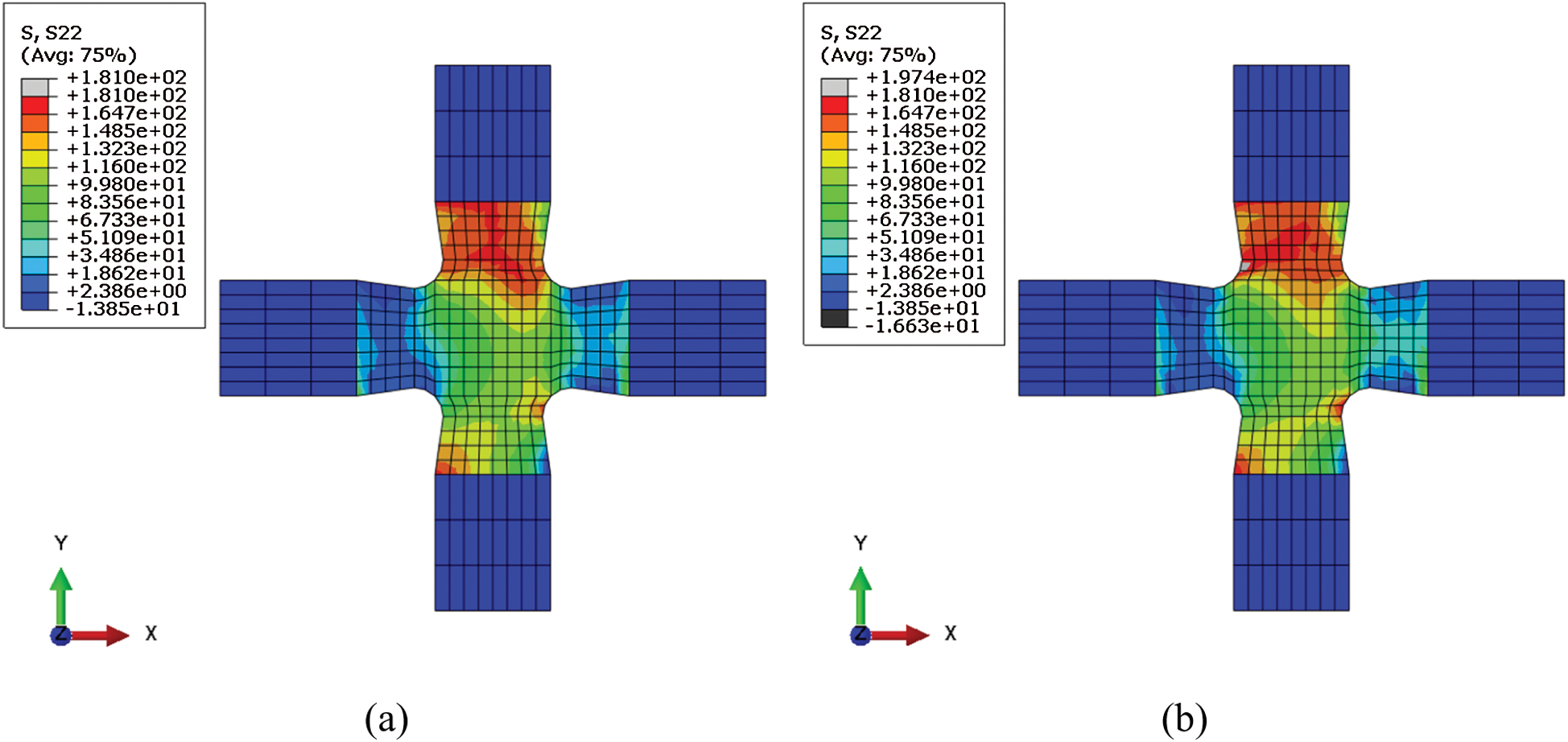
Figure 15: Stress (S22) contour comparison. (a) Result of the reference simulation and (b) result of SELIFE simulation at the last pass (the 10th pass)

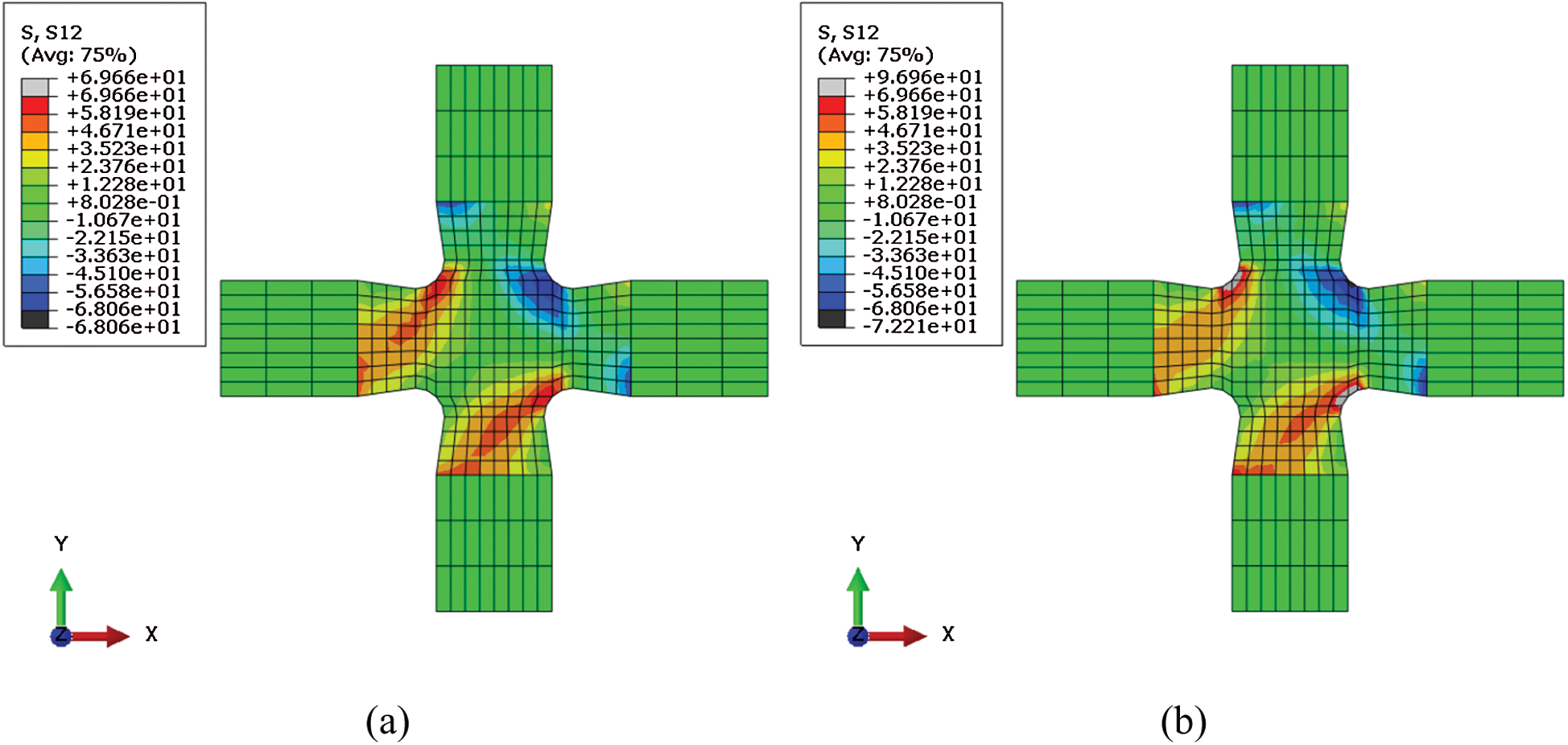
Figure 16: Stress (S12) contour comparison. (a) Result of the reference simulation and (b) result of SELIFE simulation at the last pass (the 10th pass)

The SELIFE learning progression of the elastoplastic behavior at the 132nd element is illustrated in Fig. 17. As the SELIFE DLNN pass increases, the stress-strain curves approach the reference curves. These results show promising evidence of the SELIFE performance that can learn nonlinear constitutive relationship from the experimentally measured global responses. These inverse learning results are followed by the identification algorithm to pinpoint failure initiation.

Figure 17: Stress-strain curves at the 3rd gauss point in the 132nd element by SELIFE DLNN passes

5.3 Identification of Failure Stress

By the proposed identification algorithm in Section 4.1, initial failure points were identified. As shown in Fig. 18, the identified failure points are indicated on the stress-strain curves with the failure points by Hill’s anisotropic failure criterion. The initial yield points satisfying Hill’s 48 anisotropic yield surface are exactly matching with yield points obtained by the proposed identification algorithm. The blue circle dots on each of the stress-strain curves are the initial yield points satisfying Hill’s anisotropic failure criterion while the red asterisk dots are obtained from the identification algorithm. Although only three points are presented, the majority of the identified initial yield stresses were close to the initial yield stresses satisfying Hill’s anisotropic failure criterion, according to our tests.

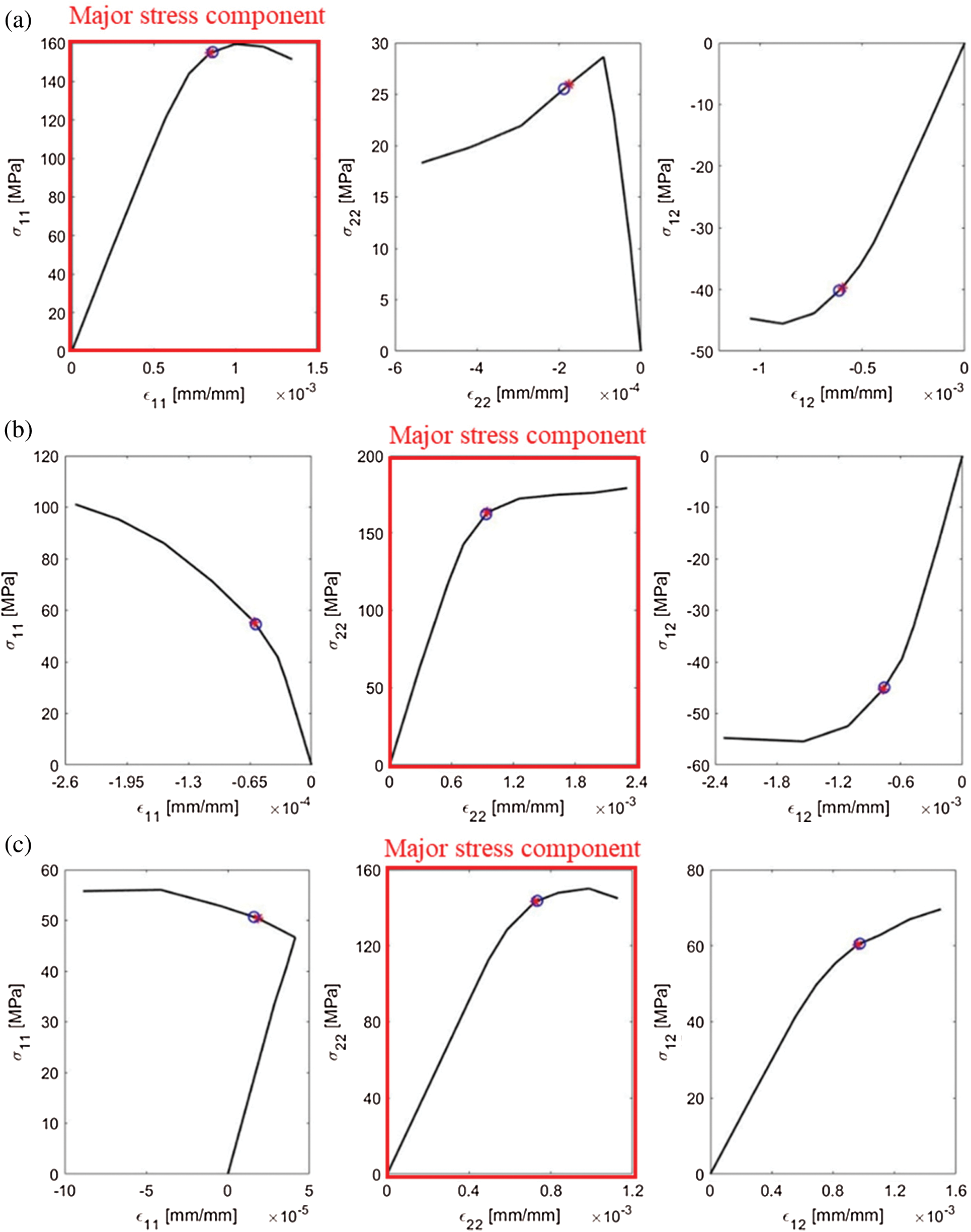
Figure 18: Comparison of the initial yield stress positions. (a) At the 2nd gauss point in the 131st element. (b) At the 2nd gauss point in the 184th element, and (c) at the 2nd gauss point in the 240th element

For example, in the case of Fig. 18a, the 11 stress component was the dominant one having maximum value and the initial yield stress was identified only with the 11 stress path. Next, the specific point within the path was saved and shared for the paired other stress component values (e.g., 22 and 12 components).

Following the feasibility study of the failure identification algorithm, two groups of the initial yield stresses were identified from all reference simulations and the self-learned stress-strain curves, respectively. Furthermore, all identified initial yield stresses, and their paired stress components were substituted into the Hill’s anisotropic failure criterion Eq. (23).

where indicates the identified initial yield stresses from the self-learned stress-strain curves.

Multiaxial stress states corresponding to the initial failure points from the self-learned stress-strain data are well-plotted on the anisotropic yield surface as shown in Fig. 19a. Moreover, the histogram of the difference defined in Eq. (23) in Fig. 19b indicates that most of the initial yield stresses are reasonably located on Hill’s anisotropic yield surface. The average percent of the error distribution is 4.0654%. These results indicate fairly good agreement owing to the failure identification algorithm and auto-adaptive algorithm.

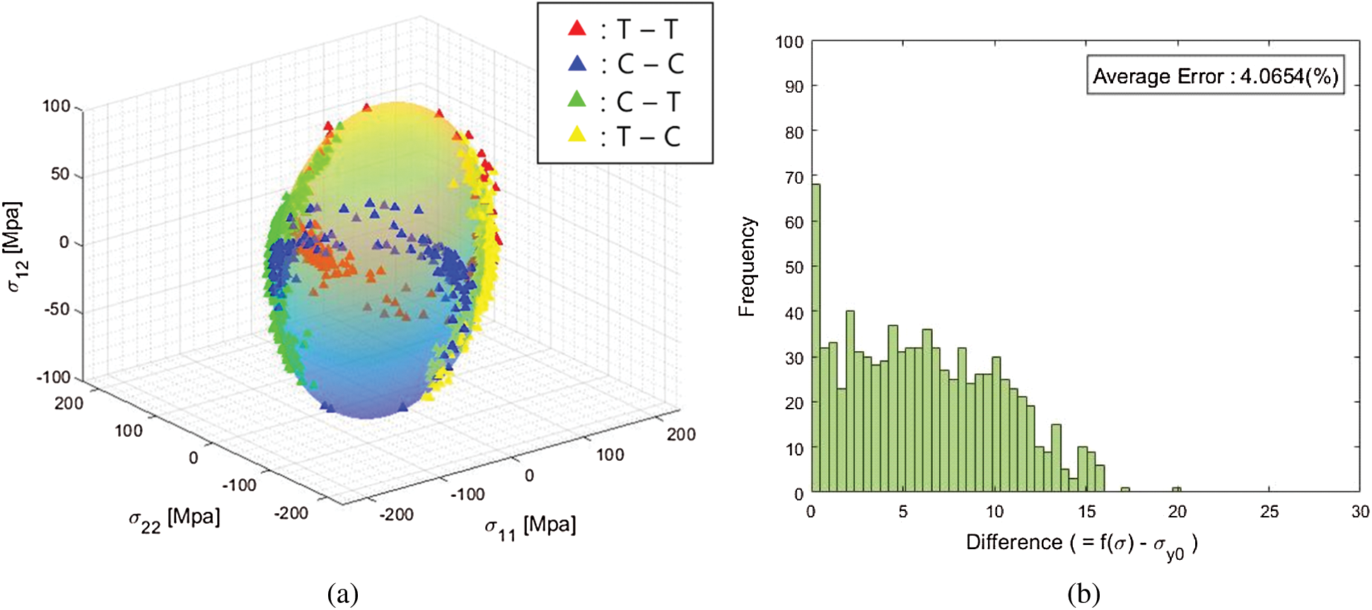
Figure 19: The identified initial yield stresses from all SELIFE stress-strain data. (a) Identified initial yield stresses on the Hill’s yield surface. (b) Distribution of errors of the identified initial yield stresses in Eq. (23)

5.5 Development of Data-Driven Failure Criterion by Genetic Programming

The failure dataset is prepared from all SELIFE simulations. We name the yield surface as a “self-learning data-driven yield surface”. Furthermore, the data-driven yield surfaces are compared with Hill’s anisotropic yield surface to verify the feasibility of the data-driven failure modeling methodology. Anisotropic constant parameters ( and ) from the Hill’s 48 anisotropic failure criterion should be determined by multiple experimental specimen tests.

However, the proposed self-learning data-driven methodology has a unique advantage of formulating anisotropic failure criterion without and constants from a minimal number of experimental tests. We explain how to prepare training data to be used in the data-driven failure criteria modeling. Assuming a quadratic strength relationship, a general anisotropic failure criterion can be expressed as

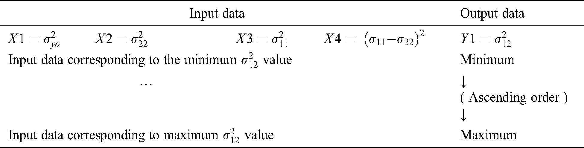
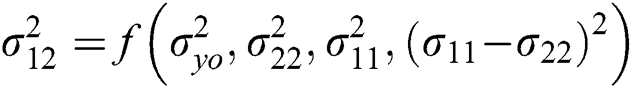
where indicates the initial yield stress of the given material and indicates the identified initial yield stresses. It is worth noting that and constants are not included in Eq. (24). The inputs to the GP training are combinations of quadratic terms of the normal stresses (), shear stress () and initial yield stress (). was chosen as output of the general failure criterion. The input and output patterns for the GP training are summarized in Tab. 12.

Table 12: Input and output data pattern for the genetic program

Several parameters associated with the GP training are shown in Tab. 13 and the operational functions are shown in Tab. 14. The initial yield stress dataset was prepared by the proposed method and trained under the same conditions as in Tabs. 13 and 14.

Table 13: Parameters for genetic program

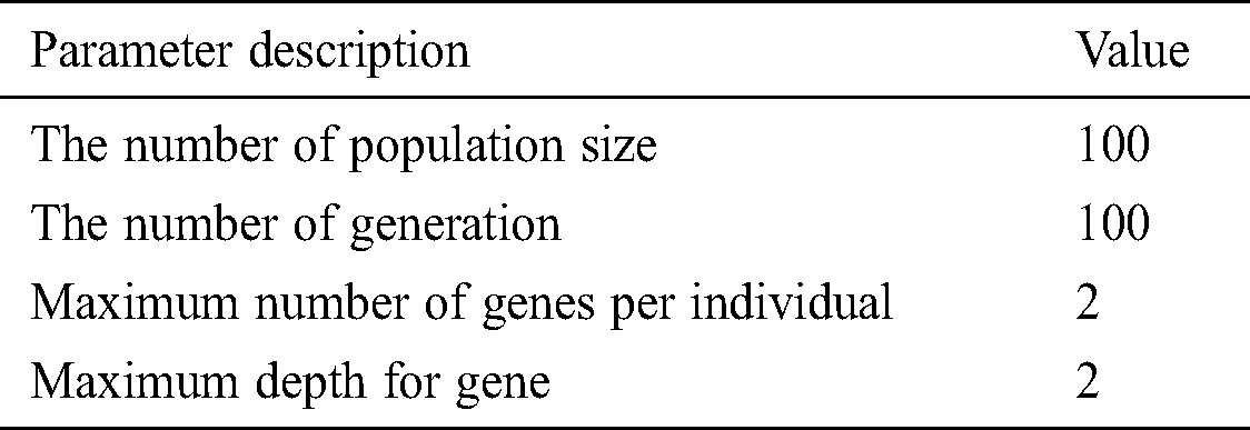
Table 14: Activated functions for the genetic programming

Finally, the GP symbolic regression was conducted with the database from all the SELIFE simulations. The data-driven anisotropic failure criterion is obtained as

Eq. (25) can produce a reasonable elliptic shape. The self-learning data-driven anisotropic yield surface Eq. (25) was compared with the reference Hill’s 48 yield surface in Figs. 20a and 20b.

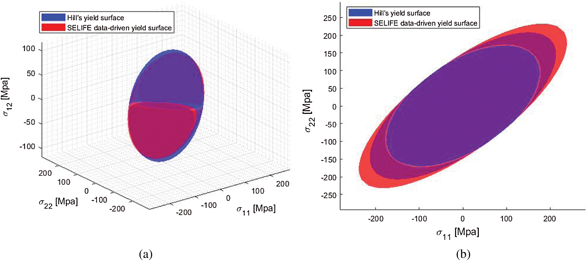
Figure 20: Comparison of the self-learning data-driven anisotropic yield surfaces with Hill’s yield surface. (a) 3D stress space. (b) 2D stress plane

The present results are promising and innovative in the fact that the anisotropic yield surface of unknown material can be developed by using the minimal number of experimental tests.

5.6 Verification of the Self-Learning Data-Driven Failure criterion

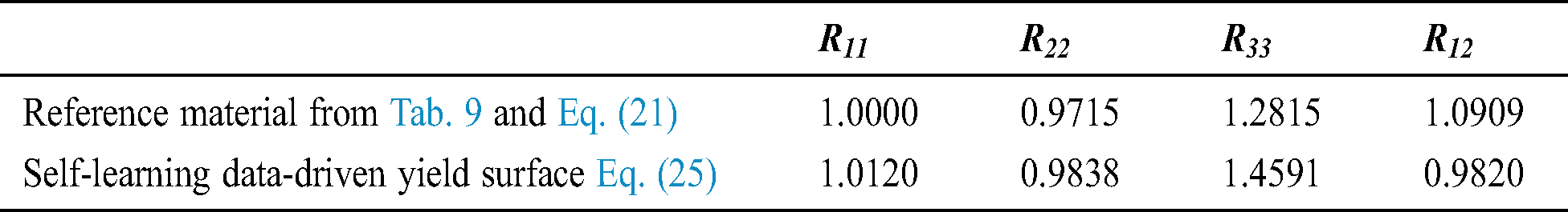
Based on the anisotropic parameters ( and ) of the data-driven yield surface i.e., Eq. (25), measured yield stresses are back-calculated. Then, yield stress ratios (, , and ) were calculated by Eq. (18) and are listed in Tab. 15. Comparing with the reference yield stress ratios, yield stress ratios from the self-learning data-driven yield surface seem reasonably identical.

Table 15: Comparisons of yield surface ratios for the reference yield surface and the self-learning data-driven yield surface (, ,, and )

To verify the data-driven yield equations, additional simulations were conducted with different material orientations. In this study, we used a 22.5 degree of material orientation. The back-calculated anisotropic yield stress ratios in Tab. 15 were used for the verification simulations. Fig. 21 shows comparisons of global response under type 1 DBC for the two different anisotropic yield surfaces. Then, force-displacement data were extracted from Region A and B.

Figure 21: Force-displacement comparison from (a) the Region A and (b) the Region B

Moreover, stress-strain data were obtained from the specific elements and those are shown in Fig. 22. Comparing stress-strain curves, initial yield points from the self-learning data-driven yield surface are very close to those from the reference anisotropic yield surface. These results indicate that the proposed methodology can develop the data-driven failure criteria of unknown materials from experimental measurements.

6  Conclusions

This paper presented a novel self-learning data-driven modeling methodology that can develop failure criteria of an unknown anisotropic ductile material. The methodology consists of the DLNN-based material constitutive model, the self-learning inverse finite element (SELIFE) simulation, failure identification algorithm through data-processing, and derivation of failure criteria through symbolic regression genetic programming (GP). The SEFIFE can gradually train the DLNN material constitutive model to follow true nonlinear stress-strain relationship being guided by the experimental measurements. In particular, stress update and the algorithmic tangent operator were derived in terms of DLNN parameters to be used in nonlinear finite element codes.

1.    The DLNN material constitutive model was superior to the artificial neural network (ANN) based model in terms of computational efficiency and prediction accuracy. The DLNN material constitutive model could extend learning capabilities with massively hidden networks owing to the Leaky-ReLU activation function.

2.    The SELIFE simulation renders the DLNN material constitutive model to self-learn multiaxial nonlinear stress-strain relationship with inputs of experimentally measured boundary reaction forces and displacements. Local stress distributions and the global responses of the self-learning model were fairly close to those of the reference model. Computational procedures for the SELIFE simulation were also presented in pseudocodes.

3.    Identification techniques of the failure points based on tangent stiffnesses could reasonably pinpoint the failure points.

4.    Finally, the GP application technique were presented to develop anisotropic failure criteria of unknown anisotropic ductile materials.

5.    The proposed idea was verified by direct comparisons with the reference simulation results with Hill’s 48 anisotropic failure criteria and further tests with material having different material orientations.

The proposed methodology has significances in capabilities of developing failure criteria of uncharacterized materials such as 3D printed materials having process-dependent properties. Beyond the generalization of the self-learned DLNN model, it can also construct material-related “Big Data.” The proposed methodology can also be extended to discover damage evolution laws in the future.

Funding Statement: This work was supported by the National Research Foundation of Korea (NRF) grant of the Korea government (MSIP) (2020R1A2B5B01001899) (Grantee: GJY, http://www.nrf.re.kr) and Institute of Engineering Research at Seoul National University (Grantee: GJY, http://www.snu.ac.kr). The authors are grateful for their supports.

Conflicts of Interest: The authors declare that they have no conflicts of interest to report regarding the present study.

References

1.   J. Ghaboussi, D. A. Pecknold, M. Zhang and R. M. Haj-Ali. (1998). “Autoprogressive training of neural network constitutive models,” International Journal for Numerical Methods in Engineering, vol. 42, no. 1, pp. 105–126. [Google Scholar]

2.   C. Settgast, G. Hütter, M. Kuna and M. Abendroth. (2020). “A hybrid approach to simulate the homogenized irreversible elastic-plastic deformations and damage of foams by neural networks,” International Journal of Plasticity, vol. 126, pp. 102–624. [Google Scholar]

3.   A. Oishi and G. Yagawa. (2017). “Computational mechanics enhanced by deep learning,” Computer Methods in Applied Mechanics and Engineering, vol. 327, pp. 327–351. [Google Scholar]

4.   M. A. Bessa, R. Bostanabad, Z. Liu, A. Hu, D. W. Apley et al. (2017). , “A framework for data-driven analysis of materials under uncertainty: Countering the curse of dimensionality,” Computer Methods in Applied Mechanics Engineering, vol. 320, pp. 633–667. [Google Scholar]

5.   B. A. Le, J. Yvonnet and Q. C. He. (2015). “Computational homogenization of nonlinear elastic materials using neural networks,” International Journal for Numerical Methods in Engineering, vol. 104, no. 12, pp. 1061–1084. [Google Scholar]

6.   G. J. Yun, J. Ghaboussi and A. S. Elnashai. (2008). “A new neural network-based model for hysteretic behavior of materials,” International Journal for Numerical Methods in Engineering, vol. 73, no. 4, pp. 447–469. [Google Scholar]

7.   T. Furukawa and G. Yagawa. (1998). “Implicit constitutive modeling for viscoplasticity using neural networks,” International Journal for Numerical Methods in Engineering, vol. 43, pp. 195–219. [Google Scholar]

8.   R. Haj-Ali and H. K. Kim. (2007). “Nonlinear constitutive models for FRP composites using artificial neural networks,” Mechanics of Materials, vol. 39, no. 12, pp. 1035–1042. [Google Scholar]

9.   Z. Zhang and K. Friedrich. (2003). “Artificial neural networks applied to polymer composites: A review,” Composites Science and Technology, vol. 63, no. 14, pp. 2029–2044.

10. H. El Kadi. (2006). “Modeling the mechanical behavior of fiber-reinforced polymeric composite materials using artificial neural networks—A review,” Composite Structures, vol. 73, no. 1, pp. 1–23. [Google Scholar]

11. Y. Shen, K. Chandrashekhara, W. F. Breig and L. R. Oliver. (2004). “Neural network based constitutive model for rubber material,” Rubber Chemistry and Technology, vol. 77, no. 2, pp. 257–277. [Google Scholar]

12. B. Wang, J. H. Ma and Y. P. Wu. (2013). “Application of artificial neural network in prediction of abrasion of rubber composites,” Materials & Design, vol. 49, pp. 802–807. [Google Scholar]

13. S. Jung and J. Ghaboussi. (2006). “Characterizing rate-dependent material behaviors in self-learning simulation,” Computer Methods in Applied Mechanics and Engineering, vol. 196, no. 1–3, pp. 608–619. [Google Scholar]

14. T. Furukawa and G. Yagawa. (1998). “Implicit constitutive modelling for viscoplasticity using neural networks,” International Journal for Numerical Methods in Engineering, vol. 43, no. 2, pp. 195–219. [Google Scholar]

15. R. M. Diaconescu, M. Barbuta and M. Harja. (2013). “Prediction of properties of polymer concrete composite with tire rubber using neural networks,” Materials Science and Engineering B-Advanced Functional Solid-State Materials, vol. 178, no. 19, pp. 1259–1267. [Google Scholar]

16. A. M. Hassan, A. Alrashdan, M. T. Hayajneh and A. T. Mayyas. (2009). “Prediction of density, porosity and hardness in aluminum–copper-based composite materials using artificial neural network,” Journal of Materials Processing Technology, vol. 209, no. 2, pp. 894–899. [Google Scholar]

17. V. M. Nguyen-Thanh, X. Zhuang and T. Rabczuk. (2020). “A deep energy method for finite deformation hyperelasticity,” European Journal of Mechanics a-Solids, vol. 80, pp. 103–874. [Google Scholar]

18. K. Wang and W. C. Sun. (2019). “Meta-modeling game for deriving theory-consistent, microstructure-based traction-separation laws via deep reinforcement learning,” Computer Methods in Applied Mechanics and Engineering, vol. 346, pp. 216–241. [Google Scholar]

19. Z. Liu and C. T. Wu. (2019). “Exploring the 3D architectures of deep material network in data-driven multiscale mechanics,” Journal of the Mechanics and Physics of Solids, vol. 127, pp. 20–46. [Google Scholar]

20. M. Raissi and G. E. Karniadakis. (2018). “Hidden physics models: Machine learning of nonlinear partial differential equations,” Journal of Computational Physics, vol. 357, pp. 125–141. [Google Scholar]

21. J. Sirignano and K. Spiliopoulos. (2018). “DGM: A deep learning algorithm for solving partial differential equations,” Journal of Computational Physics, vol. 375, pp. 1339–1364.

22. J. Berg and K. Nystrom. (2018). “A unified deep artificial neural network approach to partial differential equations in complex geometries,” Neurocomputing, vol. 317, pp. 28–41.

23. H. Guo, X. Zhuang and T. Rabczuk. (2019). “A deep collocation method for the bending analysis of kirchhoff plate,” Computers, Materials & Continua, vol. 59, no. 2, pp. 433–456.

24. C. Anitescu, E. Atroshchenko, N. Alajlan and T. Rabczuk. (2019). “Artificial neural network methods for the solution of second order boundary value problems,” Computers, Materials & Continua, vol. 59, no. 1, pp. 345–359. [Google Scholar]

25. E. Weinan and B. Yu. (2018). “The deep ritz method: A deep learning-based numerical algorithm for solving variational problems,” Communications in Mathematics and Statistics, vol. 6, no. 1, pp. 1–12. [Google Scholar]

26. I. E. Lagaris, A. Likas and D. I. Fotiadis. (1998). “Artificial neural networks for solving ordinary and partial differential equations,” IEEE Transactions on Neural Networks, vol. 9, no. 5, pp. 987–1000. [Google Scholar]

27. T. Kirchdoerfer and M. Ortiz. (2016). “Data-driven computational mechanics,” Computer Methods in Applied Mechanics and Engineering, vol. 304, pp. 81–101. [Google Scholar]

28. T. Kirchdoerfer and M. Ortiz. (2018). “Data-driven computing in dynamics,” International Journal for Numerical Methods in Engineering, vol. 113, no. 11, pp. 1697–1710.

29. R. Eggersmann, T. Kirchdoerfer, S. Reese, L. Stainier and M. Ortiz. (2019). “Model-free data-driven inelasticity,” Computer Methods in Applied Mechanics and Engineering, vol. 350, pp. 81–99. [Google Scholar]

30. T. Kirchdoerfer and M. Ortiz. (2017). “Data driven computing with noisy material data sets,” Computer Methods in Applied Mechanics and Engineering, vol. 326, pp. 622–641.

31. L. Stainier, A. Leygue and M. Ortiz. (2019). “Model-free data-driven methods in mechanics: Material data identification and solvers,” Computational Mechanics, vol. 64, no. 2, pp. 381–393. [Google Scholar]

32. F. Abbassi, T. Belhadj, S. Mistou and A. Zghal. (2013). “Parameter identification of a mechanical ductile damage using artificial neural networks in sheet metal forming,” Materials & Design, vol. 45, pp. 605–615. [Google Scholar]

33. A. Leygue, M. Coret, J. Réthoré, L. Stainier and E. Verron. (2018). “Data-based derivation of material response,” Computer Methods in Applied Mechanics and Engineering, vol. 331, pp. 184–196. [Google Scholar]

34. P. Ladevèze, D. Néron and P. W. Gerbaud. (2019). “Data-driven computation for history-dependent materials,” Comptes Rendus Mecanique, vol. 347, no. 11, pp. 831–844. [Google Scholar]

35. W. K. Liu, G. Karniadakis, S. Tang and J. Yvonnet. (2019). “A computational mechanics special issue on: Data-driven modeling and simulation—Theory, methods, and applications,” Computational Mechanics, vol. 64, no. 2, pp. 275–277.

36. M. Dalemat, M. Coret, A. Leygue and E. Verron. (2019). “Measuring stress field without constitutive equation,” Mechanics of Materials, vol. 136, pp. 103087.

37. L. T. K. Nguyen and M. A. Keip. (2018). “A data-driven approach to nonlinear elasticity,” Computers and Structures, vol. 194, pp. 97–115. [Google Scholar]

38. J. Ghaboussi, J. H. Garrett and X. Wu. (1991). “Knowledge-based modeling of material behavior with neural networks,” Journal of Engineering Mechanics, ASCE, vol. 117, no. 1, pp. –132~153. [Google Scholar]

39. G. J. Yun, J. Ghaboussi and A. S. Elnashai. (2008). “A new neural network-based model for hysteretic behavior of materials,” International Journal for Numerical Methods in Engineering, vol. 73, no. 4, pp. 447–469. [Google Scholar]

40. Y. M. A. Hashash, S. Jung and J. Ghaboussi. (2004). “Numerical implementation of a neural network based material model in finite element analysis,” International Journal for Numerical Methods in Engineering, vol. 59, no. 7, pp. 989–1005. [Google Scholar]

41. G. J. Yun, A. Saleeb, S. Shang, W. Binienda and C. Menzemer. (2012). “Improved selfsim for inverse extraction of non-uniform, nonlinear and inelastic constitutive behavior under cyclic loadings,” Journal of Aerospace Engineering, vol. 25, no. 2, pp. 256–272. [Google Scholar]

42. A. L. Maas, A. Y. Hannun and A. Y. Ng. (2013). “Rectifier nonlinearities improve neural network acoustic models,” in Proc. of the 30th Int. Conf. on Machine Learning, Atlanta, Georgia, USA, pp. 3. [Google Scholar]

43. D. P. Kingma and J. Ba. (2014). “Adam: a method for stochastic optimization,” . [Online]. Available: https://arxiv.org/abs/1412.6980. [Google Scholar]

44. R. Pascanu, T. Mikolov and Y. Bengio. (2013). “On the difficulty of training recurrent neural networks,” in Proc. of the 30th Int. Conf. on Machine Learning, Atlanta, Georgia, USA, PMLR, vol. 28, no. 3, pp. 1310–1318. [Google Scholar]

45. M. Abadi, A. Agarwal, P. Barham, E. Brevdo, Z. Chen et al. (2016). , “Tensorflow: Large-scale machine learning on heterogeneous distributed systems,” . [Online]. Available: https://arxiv.org/abs/1603.04467. [Google Scholar]

46. A. Géron. (2017). Book Hands-On Machine Learning with Scikit-Learn, Keras, and TensorFlow: Concepts, Tools, and Techniques to Build Intelligent Systems, Sebastopol, CA. 1st ed., O'Reilly Media. [Google Scholar]

47. K. He, X. Zhang, S. Ren and J. Sun. (2015). “Delving deep into rectifiers: Surpassing human-level performance on lmageNet classification,” in 2015 IEEE Int. Conf. on Computer Vision, Santiago, pp. 1026–1034.

48. D. P. Searson, D. E. Leahy and M. J. Willis. (2010). “GPTIPS: An open source genetic programming toolbox for multigene symbolic regression,” in Proc. of the Int. Multi Conf. of Engineers and Computer Scientists, 2010 Vol I, IMECS 2010, March 17–19, 2010, Hong Kong, pp. 77–80. [Google Scholar]

49. Y. Choi, C. S. Han, J. K. Lee and R. H. Wagoner. (2006). “Modeling multi-axial deformation of planar anisotropic elasto-plastic materials, part I: Theory,” International Journal of Plasticity, vol. 22, no. 9, pp. 1745–1764. [Google Scholar]

50. R. Hill. (1948). “A theory of the yielding and plastic flow of anisotropic metals,” Proceedings of the Royal Society of London Series a-Mathematical and Physical Sciences, vol. 193, no. 1033, pp. 281–297. [Google Scholar]

51. S. Bagherzadeh, M. J. Mirnia and B. M. Dariani. (2015). “Numerical and experimental investigations of hydro-mechanical deep drawing process of laminated aluminum/steel sheets,” Journal of Manufacturing Processes, vol. 18, pp. 131–140. [Google Scholar]

52. D. V. Hai, S. Itoh, T. Sakai, S. Kamado and Y. Kojima. (2008). “Experimentally and numerical study on deep drawing process for magnesium alloy sheet at elevated temperatures,” Materials Transactions, vol. 49, no. 5, pp. 1101–1106. [Google Scholar]

This work is licensed under a Creative Commons Attribution 4.0 International License, which permits unrestricted use, distribution, and reproduction in any medium, provided the original work is properly cited.