DOI:10.32604/cmc.2020.012986
| Computers, Materials & Continua DOI:10.32604/cmc.2020.012986 | |
| Article |
Three-Dimensional Distance-Error-Correction-Based Hop Localization Algorithm for IoT Devices
1School of Computer Science and Engineering, Lovely Professional University, Punjab, 144001, India
2Department of Computer Science and Engineering, Sejong University, Seoul, 05006, Korea
3Department of Financial Information Security, Kookmin University, Seoul, 02707, Korea
4Department of Information Contents, Kwangwoon University, Seoul, 01897, Korea
*Corresponding Author: Kwang Chul Son. Email: kcson@kw.ac.kr
Received: 21 July 2020; Accepted: 24 August 2020
Abstract: The Internet of Things (IoT) is envisioned as a network of various wireless sensor nodes communicating with each other to offer state-of-the-art solutions to real-time problems. These networks of wireless sensors monitor the physical environment and report the collected data to the base station, allowing for smarter decisions. Localization in wireless sensor networks is to localize a sensor node in a two-dimensional plane. However, in some application areas, such as various surveillances, underwater monitoring systems, and various environmental monitoring applications, wireless sensors are deployed in a three-dimensional plane. Recently, localization-based applications have emerged as one of the most promising services related to IoT. In this paper, we propose a novel distributed range-free algorithm for node localization in wireless sensor networks. The proposed three-dimensional hop localization algorithm is based on the distance error correction factor. In this algorithm, the error decreases with the localization process. The distance correction factor is used at various stages of the localization process, which ultimately mitigates the error. We simulated the proposed algorithm using MATLAB and verified the accuracy of the algorithm. The simulation results are compared with some of the well-known existing algorithms in the literature. The results show that the proposed three-dimensional error-correction-based algorithm performs better than existing algorithms.
Keywords: 3D localization; DV-hop algorithm; IoT; PSO; wireless sensor networks
Sensor nodes are a central part of Internet of Things (IoT) systems, enabling the IoT and the Industrial IoT (IIoT) by collecting, analyzing, storing, transmitting, and utilizing the data based on the application. Sensors are becoming more versatile, and they are used more and more in many IoT applications, including Industry 4.0, consumer wearables, healthcare services, and remote monitoring systems. A Wireless Sensor Network (WSN) is used in the design of the IoT for sensing the environment, collecting the data, and sending the data to the base station and to the locations used for analysis. In WSNs, sensor nodes operate together to sense the surroundings to attain a common goal. However, if a Base Station (BS) receives data from a particular event, but does not recognize where the event has happened, the BS cannot take the best action for the event. Because automation and intelligence have become prominent components of today’s technology-driven society, there is increasing demand for localization in various applications, including smart cities, smart healthcare, habitat monitoring, and military applications, among others [1–3].
Localization means the ability to discover where an event occurs. The security of the localization information is crucial for some applications, like missile target identification, disaster management, and monitoring of the elderly, among others [4]. The classic meaning of localization is to localize a sensor node in a Two-Dimensional (2D) WSN. However, in certain application areas, such as surveillance, underwater monitoring, and environmental monitoring, WSNs are deployed in a Three-Dimensional (3D) plane. While 2D uses only two planes, the x and y planes, 3D uses an additional z plane for height. 3D localization is more complex than 2D localization. There are several 2D localization schemes available in the literature; however, for 3D localization, the options are limited [5]. Global Positioning System (GPS) is the best-known localization solution; however, it requires a line of sight with a number of GPS satellites for accurate location information. The GPS system does not work effectively if electromagnetic waves are obstructed by obstacles in environments such as indoors, underwater, in dense forests, and or in urban canyons. This means that an alternative method is needed to find event locations without GPS, even if GPS is still the most accurate method [6]. In this work, we focus on developing a novel approach based on hop counts for localization with better accuracy.
In WSNs, the nodes that know their position in the network are called anchor nodes, and those that do not know their location are known as unknown nodes [7]. In general, most localization algorithms are classified into two categories: range-based and range-free localization algorithms [8]. Range-based localization algorithms are always restricted in terms of hardware requirements, and primarily use parameters like Received Signal Strength Indicator (RSSI), Time of Arrival (TOA), Time Difference of Arrival (TDOA), etc. This approach is vulnerable to noise and signal fading and may lose some of the information. On the other hand, range-free localization algorithms use the connectivity and hop count values as a parameter. The main challenge with this approach is accuracy. Although range-free localization is less accurate than 2D algorithms, this is a cost-effective method without restrictive hardware requirements.
Consequently, we sought to find a range-free localization approach with greater accuracy in the 3D environment. While there has been a lot of research on the 2D environment, the 3D environment is actually where most of the real-world applications work. Working in the 3D environment is challenging, as it requires more complicated computations. In the last decade, much work has been done on hop-based algorithms, but there are still many issues related to accuracy and complexity. In this work, we propose an approach to enhance the accuracy of traditional hop-based algorithms for 3D environments. The proposed Three-Dimensional Distance-Error-Correction-based hop (3D-DECHop) localization algorithm is based on the distance error correction factor. The main contributions of the paper are as follows.
i) It proposes a distributed and range-free 3D localization algorithm based on the error correction factor for the hop-based localization system. The proposed algorithm mitigates error and increases accuracy.
ii) The proposed approach is compared to the basic hop-based approach through empirical analysis to demonstrate its effectiveness.
iii) An extensive assessment of the proposed approach and comparisons with other established algorithms of a similar nature are presented.
In this section we discuss some of the 3D localization algorithms reported in the literature. Localization for the 3D environment has been studied less than that for the 2D environment. One of the major challenges of the 3D localization algorithm is accuracy. There are several 3D localization algorithms that are well studied, such as Approximation Point in Triangle (APIT), centroid, amorphous, Multi Dimensional Scaling (MDS), grid scan, and Distance Vector hop (DV-Hop). Researchers have focused mainly on DV-Hop-based approaches because they are simpler and require less hardware. In general, a modified 3D DV-Hop approach depends on the error correction factor.
Chen et al. [9] proposed a centroid localization algorithm for 3D WSNs. This algorithm has three steps. First, every anchor passes the coordinate data to other sensor nodes in the same field. Every unknown node gets the detailed coordinates of the various anchor nodes. In the second step, an unknown node selects any four anchors within its range value form the tetrahedron. In the third step, nodes use the centroid theorem on the tetrahedron. This scheme is promising for 3D WSN applications. However, the localization error in this approach is very high and accuracy is low.
Yang et al. [10] presented a 3D Voronoi diagram-based sequence localization correction algorithm called SLC3V. This algorithm uses a Voronoi diagram for dividing the 3D location space to build a rank sequence table. SLC3V uses the RSSI method between beacon nodes as a reference to correct the measured distance. The authors deploy the beacon nodes randomly in a 3D cube for simulation. The simulation results show that this algorithm can improve localization accuracy for sensor nodes in complex 3D space with fewer measurements and fewer computational costs. Singh et al. [11] proposed a 3D node localization algorithm using Computational Intelligence (CI) for moving target nodes in an anisotropic network. CI applications, i.e., Particle Swarm Optimization (PSO), H-best Particle Swarm Optimization (HPSO), Biogeography-Based Optimization (BBO), and the Firefly Algorithm (FA), are used to estimate the optimum location of nodes. Each node is assumed to have a heterogeneous property due to residual battery status. Whenever a target moving node comes within range of the anchor, the projection method is used to find its position. This algorithm can be used in various harsh environment applications and in rescue operations in hostile areas.
Another approach based on the multidimensional scaling technique for 3D node localization in a WSN is proposed by Stojkoska [12]. In this work, the author used the heuristic methods for distance calculation. One of the limitations of this approach is that it does not perform well in complex deployment scenarios with irregular topologies. 3PDHDV-Hop is another approach, proposed by Wang et al. [13], which uses the partial value instead of the average value of the hop size in a 3D network environment. It reduces error and improves accuracy by selecting the projection plane. A localization based on the Gauss–Newton method is developed for 3D WSNs to improve the coordinate estimation [14]. This algorithm delivers better outcomes compared to other DV-Hop-based algorithms, which use the least square technique for position estimation. Ahmad et al. [15] proposed a scheme called Parametric Loop Division (PLD). In this algorithm, the sensor node position is calculated with the support of anchor nodes deployed in the form of a ring matrix. Compared to APIT, DV-Hop, and MDS algorithms, this scheme has low computation costs and low complexity. Yi et al. [16] proposed a hybrid approach based on APIT and DV-Hop. The APIT and DV-Hop algorithms are merged, and a new hybrid approach is formulated for improving localization accuracy with large coverage. The localization accuracy in dense environments is increased using triangles in the triangle interior point test (PIT) by selecting good triangles. The simulation results show that this hybrid algorithm can improve localization accuracy in a dense environment and increase location coverage of beacon nodes in a sparse environment.
Chen et al. [17] proposed a PSO-based 3D localization algorithm to mitigate the challenges of the basic DV-Hop algorithms. This approach is more effective and has less cost involved in the computation. Another algorithm for 3D space, called particle-based improved DV-Hop (PMDV-Hop), is proposed for the real-world environment [18]. In this algorithm, the average distance per hop of the anchor nodes is calculated by RMSE and is dynamically corrected with weighted RMSE. The PSO of intelligent optimization algorithms is applied to an MDV-Hop localization algorithm, called PMDV-hop. In this algorithm, the inertia weight and trust coefficient are calculated dynamically. An enhanced DV-Hop algorithm, which depends on cuckoo search to increase effectiveness in terms of error and precision values, is presented by Zhang et al. [19]. This approach uses an adaptive bird nest and step search technique to increase the convergence percentage of the algorithm. One of the challenges not addressed by this algorithm is the un-organized distribution of anchor nodes (which is accommodated by our proposed approach). It is because in our proposed approach there is no fixed position deployment of nodes whereas in the former one, they have deployed the nodes at some fixed positions. In our proposed approach random distribution models are used for deploying the nodes.
Some variations of the algorithms discussed above are presented with more analysis and in an improved form in [20–24]. From these reviews we concluded that accurate localization in a 3D environment is a very challenging task, and that there is still room for improvement in this domain. Therefore, we set out to improve the accuracy of the hop-based algorithm. The environment in 3D is more complex than 2D and it is not just adding one more dimension into it. But the main challenges lie in deciding the plane of the coordinate for calculating the correct position which is the future work pertaining to the present proposed approach. Also, the proposed work can be extended with the introduction of optimization strategies for inferring more accurate insights.
3 Proposed 3D-DEC Hop Algorithm
In general, all hop-based algorithms are based on the Distance Vector (DV) approach. They include three basic steps: hop count calculation, average hop size calculation, and estimation of coordinates. First of all, the distances between the nodes are calculated using the hop count. Then hop size values are calculated for the estimation of coordinates, using any available method. During the distance calculation, there are opportunities for error accumulation, which can reduce localization accuracy. The algorithm is more prone to error when the environment is real, i.e., when the environment is 3D. In this section, we describe the proposed new 3D distance-error-correction-based hop (3D-DECHop) localization algorithm. It is based on our previous work, where we developed a distance error correction approach for 2D hop-based localization [25]. Here, the proposed approach is in 3D but there is much difference in the execution of the localization process and deployment of the nodes in the given environment.
3.1 Steps of the 3D-DECHop Approach
The proposed 3D-DECHop algorithm has the following steps:
i) Hop count calculation
ii) Modified average hop size calculation based on distance error correction
iii) Estimation of the coordinates
Representation of variables
i) (Xa, Ya, Za): Coordinates of the anchor node
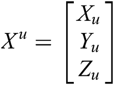
ii) (Xu, Yu, Zu): Coordinates of the unknown node
iii) h_cont: The number of hops between the sending and the receiving node
iv) tn: The total number of anchor nodes
v) average_hop_dista: Average hop distance of a particular anchor from other anchor nodes
vi) av_net_hop_dist: The average of the average hop distances of all the anchors
vii) dist_erra: The error in distance between actual coordinates using hop-based distance
viii) average_error_Anchora: An average of dist_erra
ix) total_error: The overall error from each anchor
x) distu,a: The distance between the unknown and the anchor node
In the proposed 3D-DECHop algorithm, the hop count calculation is done as in 3D DV-Hop and PSO-based 3D DV-Hop algorithms. All anchor nodes in the network broadcast the packets that contain the details of the coordinates, initially set as h_count = 0, and the ID of the node. Each node, whether it is an anchor or an unknown node, maintains the table of every anchor node. A node can receive packets from the same anchor node via different paths, because of broadcasting. Therefore, whenever a node receives the same packet, it checks the hop count. If the hop count is smaller than the previous entry in the table, the node receives the packet and updates the table hop count; otherwise it discards the packet. Eventually, every node finds the minimum hop count to every other node in the network.
3.1.2 Modified Average Hop Size Calculation
Anchor nodes use the following equation, Eq. (1), to find the average hop distance to another anchor node.
For each anchor

End
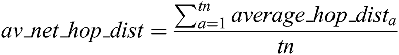
After obtaining the average hop distance, anchors broadcast the average_hop_dista. Once anchors receive and update their tables with the average_hop_dista, they calculate the average of  as
as  . While in conventional 3D DV-Hop, the average hop distance to the closest anchor node is used, in the proposed 3D-DECHop algorithm the average of the hop distance for the entire network is used, as in Eq. (2). Through the addition of the
  value, which is a modification of the traditional algorithm, the overall localization process becomes independent of the nearest anchor. The reason for this process is that the use of the average distance to the closest anchor node adds to error ambiguity in traditional DV-Hop because of variations in the actual distances between the nodes. Sometimes the average distance is greater than the absolute distance, and other times it can be smaller. To solve this issue of error ambiguity, the 3D-DECHop algorithm does not use the closest anchor average hop distance, but works in the intermediate network hop distance to find the precise hop distance, as shown in the algorithm step below.
For each anchor
End
Subsequently, the error regarding each anchor is identified as dist_erra and then calculated with Eq. (3). This defines the error value in terms of the hop distance that arises on account of the use of the average hop distance. Then the true distance is found from the multiplication of the hop distance and hop count. Afterward, the error computed in (3) is broadcast by each anchor, as defined in the algorithm step below.
For each anchor

End
Now each anchor broadcasts the error.
For each anchor,
Broadcast distance error.
End
Again, we need to estimate the average error of each anchor with other anchors through Eq. (4), as defined in the algorithm step below.
For each anchor
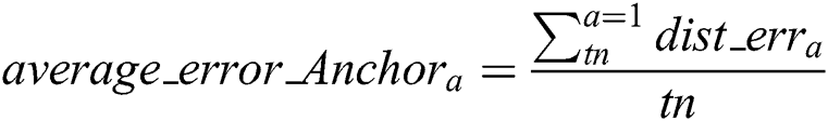
End
Now every anchor broadcasts the average error in the network. A node calculates the total error, considering all anchor nodes using (5). Now the node is able to find the intermediate error of all the anchors in the network, as mentioned in [25].
For each anchor
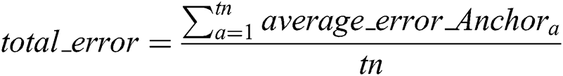
End
Finally, each unknown node finds the distance between the anchor node and other nodes through (6). Here, as in the traditional algorithms, the average network error is the cross product with the hop count, used to calculate the updated error.
Similarly, to reduce the distance error in 3D-DECHop, a product of the combined error with the hop count is subtracted from the updated distance, as per (6). The reason for multiplying the hop count with the combined error is the ambiguity in the traditional DV-Hop, where the hop count leads to error. Here, the total_error is subtracted from h_cont because it is formulated from dist_err which further contains h_cont as mentioned in Eq. (3). Hence, if the distance error is reduced, then the localization error is also noticeably reduced, and the precise result is formulated in the step below.
For every anchor
For every unknown

End
End
3.1.3 Estimation of the Coordinates
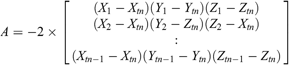
After getting the distance, the multilateration method is used to find the coordinates, as shown in Eq. (7) to (12).
For 1 to anchor -1

End
Find AX=B
For every unknown
For 1 to anchor -1

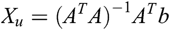
End
End
Here, AT is the value of the transpose of matrix A followed by the computation of coordinate values.
3.2 Error Analysis in 3D-DECHop
This section deals with the mathematical error analysis of the 3D-DECHop approach in comparison to traditional 3D DV-Hop by considering the scenario as shown in Fig. 1. A1, A2, A3, and A4 are anchor nodes representing the vertices of a tetrahedron, while U is unknown node. The values on the connecting lines represent the distance between the nodes, which is taken from the practical implementation of the scenario.
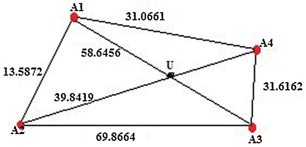
Figure 1: Node representation for error analysis in the 3D-DECHop algorithm
Step 1: Eq. (1) is used to determine the average hop distance for all the anchor nodes, as stated below. The distance is given in meters (m).
Step 2: Let us assume that U is an unknown node. The traditional DV-Hop always finds the average hop distance of the closest anchor node. In the scenario from Fig. 1, these nodes would use the average hop distance of A3, that is, 34.1747, as it is the nearest node. An unknown node then finds the distance between itself and the anchor node by following Eq. (12). A1 = (13.5872 + 31.0661 + 58.6456)/(1 + 1 + 2) = 25.8247, A2 = (13.5872 + 39.8419 + 69.8664)/(1 + 1 + 2) = 30.8239, A3 = (31.0661 + 39.8419 + 31.6162)/(1 + 1 + 1) = 34.1747, A4 = (58.6456 + 69.8664 + 31.6162)/(2 + 2 + 1) = 32.0256.

i.e., 1 × 34.1747 = 34.1747.
However, the actual distance between U and A3 is 15. In this way, the distance error causes the error in localization when the 3D DV-Hop algorithm is used.
Step 3: To reduce the distance error, we use the average of the average hop distance corresponding to every anchor of the 3D-DECHop algorithm, as in Eq. (2). Here, the unknown node relies not only on the closest anchor node, but also on the average hop distance. It has been observed that this was the main cause of the error in the basic DV-Hop approach. The average distance of the network is calculated using Eq. (13).

Every anchor then calculates the distance error, as per Eq. (3). The distance error of A1 is updated for the other anchors, as shown in Eq. (14) to Eq. (16).

Thus, dist_err(A1) = (30.7122 × 1) – 13.5872 = 17.125.

Thus, dist_err(A1) = (30.7122 × 1) – 31.0661=0.3539.

Thus,  (A1) = (30.7122 × 2) – 58 = 3.4244. Therefore, the distance error of A1 can be calculated using Eq. (4) as (17.125 + 0.3539 + 3.4244)/3 = 6.9677.
Similarly, the distance error of A2 = 0.42. The distance error of A3 = −3.1819 and the distance error of A4 = –1.6850.
Now, to calculate the total distance error, we use Eq. (5), i.e., = (6.9677 + 0.42 + (−3.1819) + (−1.6850))/4 = 0.6302.
Step 4: Calculating the distance between the unknown and the anchor node using Eq. (6), as defined in Eq. (17).

Thus,  = (1 × 30.7122) – (1 × 0.6302) = 30.01.
The actual distance between A1 and U is 32. Basic DV-Hop yields a distance of 25.8247, while the error becomes 6.176. However, with the 3D-DECHop approach, distance is 30.01 and error is 1.99. The error is smaller than with basic 3D DV-Hop.
In this section, the behavior of the proposed 3D-DECHop in algorithm is analyzed using MATLAB [26] for the Average Localization Error (ALE), Localization Mean Square Error (LMSE), Relative Position Error (RPE), Mean Localization Error (MLE), and Localization Error Ratio (LER) for the given parameters, such as the anchor node ratio, the total node amount, and the communication range. The regular model of deployment is considered for all the comparisons of 3D-DECHop with other methods.
4.1 Simulation Setup and Comparison Metrics
Localization in 3D space shows how the algorithm would perform in actual space. Fig. 2 shows the deployment of nodes in a 3D space with dimensions of 100 m × 100 m × 100 m. In this deployment scenario, there is a total of 150 nodes deployed, out of which 30 nodes are anchor nodes. The anchor nodes are shown in red. The remaining 120 nodes, shown as black diamond symbols, are the unknown nodes, whose positions are to be determined using the proposed algorithm.
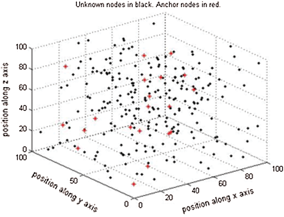
Figure 2: Node representation of the 3D-DECHop algorithm
For the comparison of the proposed 3D-DECHop algorithm with existing algorithms, some common metrics are calculated as described below.
Average Localization Error (ALE): This factor gives the variation corresponding to the actual and the estimated value of the coordinates calculated for each node in the localization process. It is defined as Eq. (18).
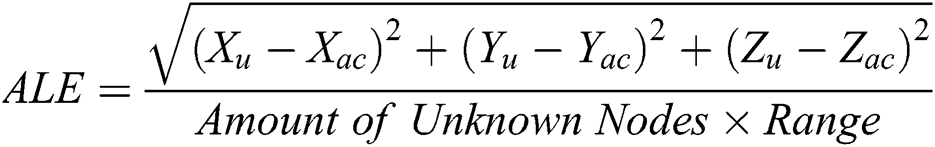
Here, Xu, Yu are the unknown node’s estimated coordinates and Xac, Yac are actual node’s coordinates. Other metrics, like RPE and LER, are computed in the same fashion as ALE. Localization error variance (LMSE): It is defined as the ratio of the average localization error to the range amount for that node. It is considered the main factor for measuring the accuracy of the localization algorithm against various parameters, such as the sensor number, the anchor node number, and the node range. It is represented as Eq. (19).
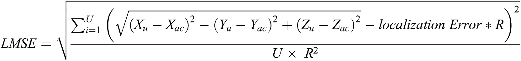
Here, U signifies the number of unknown nodes and R represents the range of each node.
Mean Localization Error (MLE): This factor gives the variation corresponding to the actual and the estimated value of the coordinates calculated for each node in the localization process. It is defined as Eq. (20).
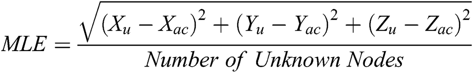
Here, Xu, Yu are the unknown node’s estimated coordinates, and Xac, Yac are the unknown node’s actual coordinates.
The analysis of the 3D-DECHop algorithm is executed through simulations in MATLAB 2013 [26]. In this section, the performance of the algorithm is assessed and compared with the existing approaches described in the literature, such as novel centroid [9], 3D DV-Hop [17], PSO-based 3D DV-Hop [17], PMDV-Hop [18], 3D-IDCP [19], 3D-OSSDL [22], DBDV-Hop [27], and ACSDV-Hop [28], using the same conditions and parameters. The results of the simulations are analyzed based on various factors, such as total number of nodes, number of anchor nodes, and node range. The simulation results are the average of 100 simulations. The selection of parameters is based on the algorithm by which our proposed approach is to be compared.
4.2.1 Comparison with Novel Centroid Localization
The 3D-DECHop algorithm is different from the basic centroid and novel centroid approaches proposed in [9]. We evaluated the algorithm in 3D space with 100 nodes deployed in a 100 m × 100 m × 100 m cube. The nodes are uniformly deployed, each within 40 m of another node. We compared the algorithms in terms of the ALE while varying the ratio of anchor nodes and the range, as shown in Figs. 3 and 4. First of all, we analyzed the amount of variation in anchor nodes in relation to the total number of nodes, as shown in Fig. 3. We can see that the error value decreases as the number of anchor nodes increases for all algorithms. This is because a higher ratio of anchor nodes to unknown nodes leads to greater availability of nodes that can assist with finding the precise position of the node of interest. It leads to more accurate localization. However, for the 3D-DECHop algorithm, the error is significantly smaller than in other algorithms. For instance, when there are 15 anchor nodes, the error for the 3D-DECHop algorithm is 0.24 m; meanwhile, centroid yields an error of 0.74 m, and novel centroid yields an error of 0.61 m. This gain in the correction metric came from the distance updating in the 3D-DECHop algorithm.
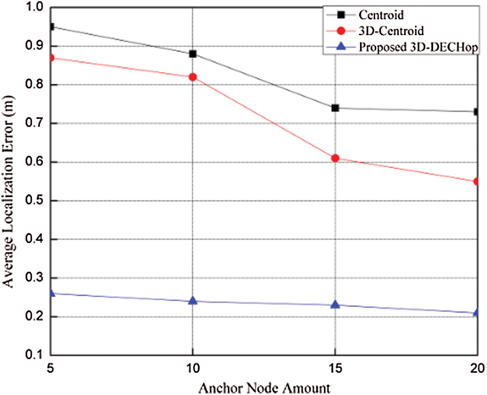
Figure 3: ALE vs. number of anchor nodes
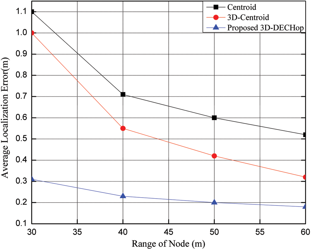
Figure 4: ALE vs. node range
Similarly, the impact of varying range on the given algorithms is shown in Fig. 4 with 100 nodes and 20 anchor nodes. It is clear that when the range of a node is increased, the error decreases for the all the algorithms considered because a greater number of nodes is available for the position assessment corresponding to the node of interest. After the range increases to 40 m, error decreases very sharply. Also, the error corresponding to a range of 40 m is 0.23 m, 0.55 m, and 0.71 m for the proposed, novel centroid, and centroid algorithms, respectively.
4.2.2 Comparison with 3D-OSSDL (Optimal Space Step Distance Localization)
The proposed algorithm is compared with the basic DV-Hop and 3D-OSSDL [29] approaches using the deployment region of 100 m × 100 m × 100 m with 250 nodes and with a range of 60 m for all nodes. The algorithms are compared based on MLE, while considering the impact of varying the anchor node number, total node number, and range, as shown in Figs. 5–7.
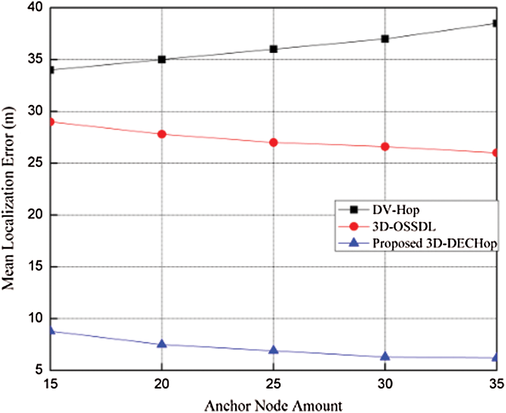
Figure 5: MLE vs. number of anchor nodes
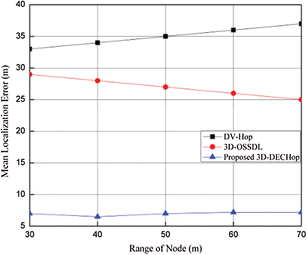
Figure 6: MLE vs. node range
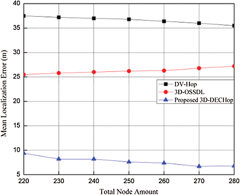
Figure 7: MLE vs. total node amount
As shown in Fig. 5, when the number of anchor nodes increases from 15 to 35, the value of the error decreases. The reason for this is similar to that discussed in Section 4.2.1. While the anchor node number is 30, the 3D-DECHop algorithm yields an error of 7 m, while the error is 27 m and 37.5 m for the DV-Hop and 3D-OSSDL algorithms, respectively. Hence, we conclude that the 3D-DECHop algorithm performs much better than the other two algorithms.
Also, when the range of the node is increased from 30 m to 70 m while keeping the total number of nodes at 250 with a 10% anchor ratio, error is eventually reduced, as shown in Fig. 6. The error corresponding to the range of 40 m is 6.8 m, 28.5 m, and 34.3 m for the proposed, DV-Hop, and 3D-OSSDL [29] algorithms, respectively. Similarly, when the number of nodes is increased, error decreases, as more nodes are available to help estimate the position of the unknown node, as shown in Fig. 7. Here, the anchor node ratio is taken as 10% of the nodes deployed, and the range is 60 m for all the nodes. The simulation results suggest that the 3D-DECHop algorithm performs much better than the other algorithms.
4.2.3 Comparison with DV-Hop-Based and Bounding Cube (DBDV-Hop) Algorithm
The 3D-DECHop algorithm is compared to the bounding cube and DBDV-Hop [29] approaches using the deployment area of 100 m × 100 m × 100 m, with 100 nodes and a range of 40 m for all nodes. The algorithms are compared based on RPEwhile considering the effect of varying the anchor node percentage and range, as shown in Figs. 8–10.
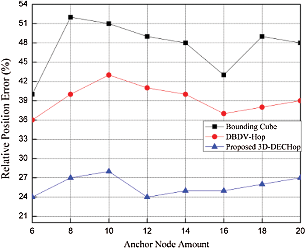
Figure 8: RPE vs. number of anchor nodes
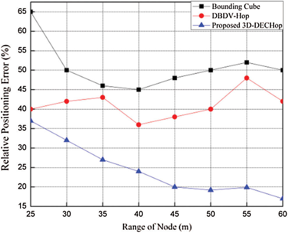
Figure 9: RPE vs. node range (anchor ratio 14%)
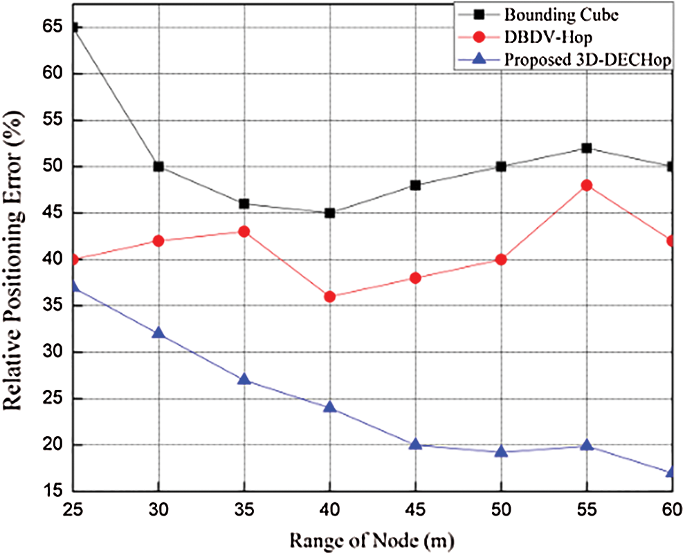
Figure 10: RPE vs. node range (anchor ratio 16%)
When the number of anchor nodes is changed from 6 to 20 with other parameters kept the same, positioning error decreases slightly at 10 anchor nodes, and then increases at 16 anchor nodes. But for the 3D-DECHop algorithm, the error variations are smaller than for the alternative algorithms; hence it is more stable and accurate. For 12 anchor nodes, the error is 0. 24 m for the proposed algorithm, as compared to 0.41 m and 0.49 m for DBDV-Hop and bounding cube, respectively. Similarly, changing the range affects the positioning error when the anchor node ratios are 14% and 16% with a total of 100 nodes, as shown in Figs. 9 and 10, respectively. As the range increases from 25 m to 60 m, in both the cases, the error value decreases. It also seems that beyond the range of 45 m, the 3D-DECHop algorithm is quite stable compared to the other algorithms.
4.2.4 Comparison with 3D DV-Hop-Based on PSO
Accuracy is one of the main factors for the assessment of various localization algorithms. It depends on the number of anchor nodes deployed. In this experiment, a total 200 nodes are implemented in the same space as in the previous comparisons. Each of these nodes has a fixed range of 30 m. To assess the performance, a LMSE value is calculated for situations where the number of anchor nodes varies from 10 to 60 nodes. Fig. 11 shows the change in the LMSE value depending on the number of anchor nodes. We conclude that the 3D-DECHop algorithm behaves better than the 3D DV-Hop and PSO-based 3D DV-Hop algorithms [17].
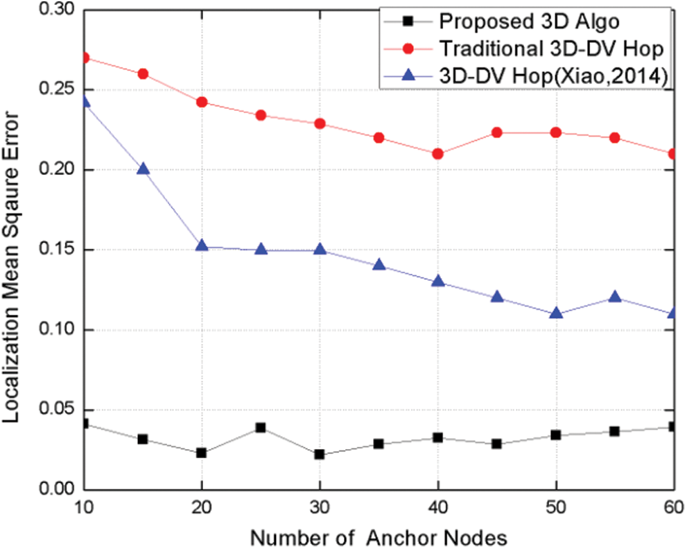
Figure 11: LMSE vs. number of anchor nodes
Fig. 11 shows that as the number of anchors raises, the LMSE value decreases for every algorithm. This is because as the number of anchor nodes rises, the count between the unknown and the anchor nodes decreases. This, in turn, further reduces the value of the hop size, which leads to the precise value of error at the end stage when error is calculated. Moreover, the average error is very limited for the 3D-DECHop algorithm in contrast to other algorithms, as per Fig. 11. This is a result of the correction factor, which is added in the 3D-DECHop approach and which further refines the dimensions of the hop size while considering the other aspects of the network.
Sensor node deployment is chosen based on the application and the environment. The number of nodes affects the accuracy of the localization algorithms. Here, the number of sensor nodes has been increased from 100 to 400 for the space measuring 100 m × 100 m × 100 m. Each node has a range of 30 m, and the number of anchor nodes is fixed at 40. To assess the performance, a LMSE value is calculated for every number for nodes between 100 and 400. Fig. 12 shows the change in the value of LMSE with the number of sensor nodes. The simulation outcomes show that with these parameters, the 3D-DECHop algorithm does better than 3D DV-Hop [17] and PSO-based 3D DV-Hop algorithms.
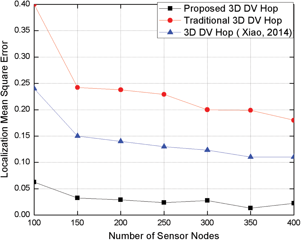
Figure 12: LMSE vs. number of deployed nodes
Fig. 12 shows that with an increase in the number of sensor nodes, the value of LMSE decreases for all the algorithms. This is because with the increase in the number of sensor nodes, connectivity value among the nodes also increases. This, in turn, provides more data on the location of nodes, and thus enhances the performance of the whole network. It is also shown that after a certain number of sensor nodes (200 nodes in Fig. 12), the variation in the localization error becomes significantly smaller; hence the algorithm is more stable and has higher precision and accuracy than the others.
The range value of the node is also one of the main factors for evaluating the accuracy of the given algorithm. Here the number of sensor nodes is fixed at 100 in the space measuring 100 m × 100 m × 100 m. The range value is allowed to vary from 22 m to 40 m for measuring the accuracy of the algorithm, while the number of anchor nodes is fixed at 30. Afterward, the LMSE value is calculated for range values from 22 m to 40 m. Fig. 13 shows the change in LMSE value in response to variation in the range value. It shows that with these parameters, 3D-DECHop algorithm behaves better than 3D DV-Hop and PSO-based 3D DV-Hop algorithms.
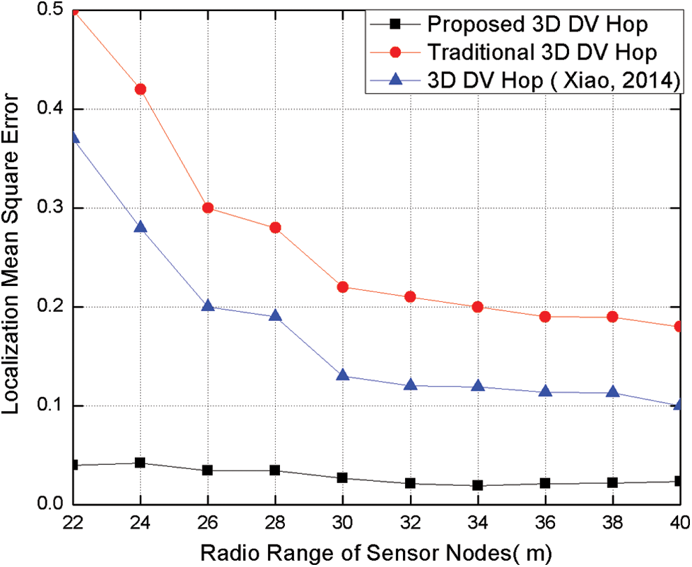
Figure 13: LMSE vs. node range
Fig. 13 clearly shows that with an increase in the range value, the LMSE value decreases for all the algorithms. The reason is that more nodes would come within range of each node and thus boost the connectivity value. This further increases the accuracy, as stated before. We can see that there is very little variation in the LMSE value with the change in the range value for the 3D-DECHop algorithm compared to the other algorithms. As in Fig. 13, the error value stabilizes after the range of 30 m, but in our case the error variation is much smaller even at the start with a range of 22 m. Hence, we conclude that range value variation has a much smaller effect on the LMSE for the proposed algorithm. This is one of the advantages of the proposed algorithm.
4.2.5 Comparison with Improved 3D Localization Algorithm
The proposed algorithm is compared with 3DV-Hop, 3DV-Distance, and 3D-IDCP [19] approaches with a deployment region of 100 m × 100 m × 100 m and with 100 nodes with a range of 40 m for all the nodes. We compared the algorithms based on the LERwhile considering the impact of varying the anchor ratio, as shown in Fig. 14. The outcomes show that the error ratio decreases for all the algorithms when the anchor node ratio increases. This is due to the extra nodes that are accessible to the unknown node for estimating its position coordinates. Still, the 3D-DECHop algorithm does better than the alternative algorithms. For example, when the anchor node ratio is 25%, the error is 0.2 m for the 3D-DECHop algorithm and 0.65 m, 0.59 m, and 0.55 m for the 3DV-Hop, 3DV-Distance, and 3D-IDCP algorithms, respectively.
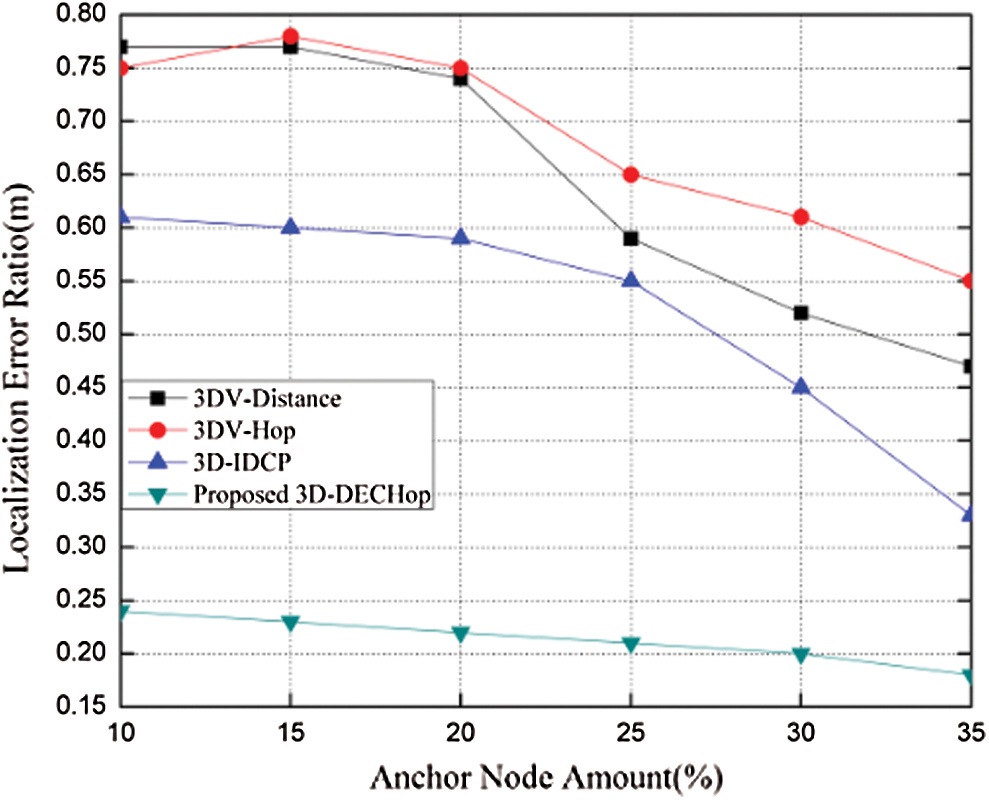
Figure 14: LER vs. number of anchor nodes
4.2.6 Comparison with Adaptive Cuckoo Search
The proposed algorithm is contrasted with traditional DV-Hop, ADV-Hop, and ACSDV-Hop [28] approaches using the deployment region of 100 m × 100 m × 100 m with 200 nodes and a range of 30 m for all the nodes. We compared the algorithms based on ALE while considering the impact of varying the anchor node ratio, the range, and the total number of nodes, as shown in Figs. 15–17. The impact of varying the number of anchor nodes on the error is shown in Fig. 15, where it is clear that when the number of anchor nodes increases, the error decreases for all the algorithms. For example, with 30 anchor nodes, the error is 1.4 m for the 3D-DECHop algorithm, and 3.4 m, 2.4 m, and 1.7 m for the traditional DV-Hop, ADV-Hop, and ACSDV-Hop algorithms, respectively.
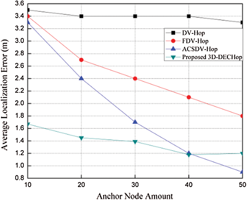
Figure 15: ALE vs. number of anchor nodes
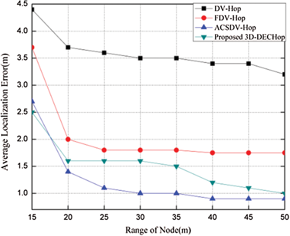
Figure 16: ALE vs. node range
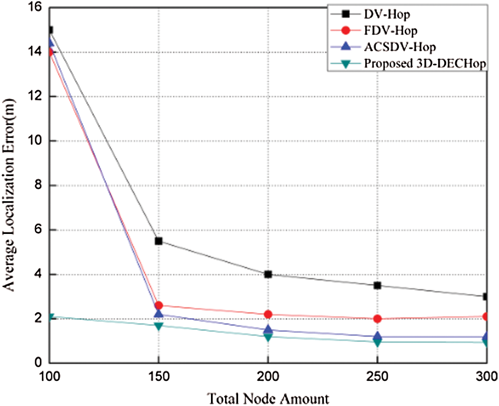
Figure 17: ALE vs. number of nodes
Similarly, when the node range is increased from 15 to 50 with 200 nodes and a 25% anchor node ratio, as shown in Fig. 16, the error decreases as the range increases. This happens because a greater number of nodes comes within range of each node as the range is increased. It is also shown that after the range reaches 20 m, the error stabilizes for all the algorithms. Nevertheless, the error for the proposed algorithm is smaller than for the other algorithms for all range values. This is also the case when the number of nodes varies from 100 to 300 with an anchor ration of 20% and a range of 30 m, as shown in Fig. 17. Once the number of nodes deployed exceeds 200, there is a marginal shift in error for all the algorithms, but 3D-DECHop still performs better than the other algorithms. Also, the deviation for the 3D-DECHop algorithm much smaller than for all the other algorithms. Moreover, in the transition from 100 to 200 nodes, error does not decline abruptly, as with the other algorithms.
4.2.7 Comparison with PSO-Based Improved DV-Hop (PMDV-Hop)
The 3D-DECHop algorithm is compared with MDV-Hop, PDV-Hop, and PMDV-Hop [18] approaches using the deployment region of 100 m × 100 m × 100 m with 200 nodes and a range of 30 m for all the nodes. We compared the algorithms based on ALE while considering the impact of varying the number of anchor nodes and the range, as shown in Fig. 18. First of all, we analyzed the effect of the anchor node ratio by varying it from 5% to 20%, as shown in Fig. 18.
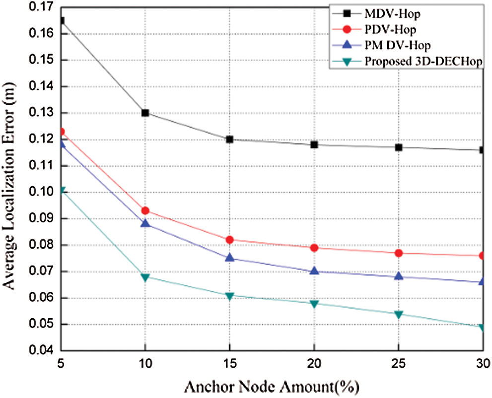
Figure 18: ALE vs. number of anchor nodes
It is clear that for all the algorithms there is a smooth decline in the error above the anchor node ratio of 20%. For the 3D-DECHop, the error reduction is greater than for the others. Also, when the range is varied from 20 m to 60 m with 200 nodes and a 15% anchor ratio, the error decreases for all the algorithms up to a range of 40 m, and then increases again as nodes communicate with each other. But in the case of the 3D-DECHop algorithm, the decline in error continues even after the range of 40 m.
Localization plays an important role in the IoT and in real-world applications of wireless sensor networks. In this work we propose a new hop-based algorithm suitable for the 3D environment, called 3D-DECHop. This algorithm is distributed and based on our previous work with the 2D environment. The accuracy of the algorithm is evaluated based on the minimum error generated during localization process. The correction factor is introduced and utilized during the various stages of the localization process, ultimately reducing the error to a large extent. In the proposed 3D-DECHop algorithm, the hop size is customized so that less error occurs. The algorithm incurs average error, unlike the separate node error in traditional DV-Hop algorithms, eventually leading to more accurate calculations. Simulation results show that the 3D-DECHop algorithm outperforms other existing algorithms, yielding lower error levels with various specifications, such as the number of nodes, the number of anchor nodes, and the range. The 3D-DECHop algorithm performs at its best when the anchor ratio is one fifth of the total number of nodes and the range is 40 m. In the future, we hope to prove the accuracy of the proposed algorithm both through an analytical approach and through experiments. Optimization can also make more preciseness in the localization error. Moreover, localization is a practical problem and it will add more essence when the experiments are conducted in the real environment. It will increase the credibility of the proposed work and we will try to execute the same in the near future.
Funding Statement: The present research has been conducted by the Research Grant of Kwangwoon University in 2020.
Conflicts of Interest: The authors declare that they have no conflicts of interest to report regarding the present study.
1. S. Y. Nam and G. P. Joshi. (2017). “Unmanned aerial vehicle localization using distributed sensors,” International Journal of Distributed Sensor Networks, vol. 13, no. 9, pp. 1–8. [Google Scholar]
2. H. Habibzadeh and T. Soyata. (2020). “Toward uniform smart healthcare ecosystems: A survey on prospects, security, and privacy considerations,” in Connected Health in Smart Cities. Berlin, Germany: Springer International Publishing, pp.75–112. [Google Scholar]
3. A. Giri, S. Dutta and S. Neogy. (2020). “Fuzzy logic-based range-free localization for wireless sensor networks in agriculture,” in Advances in Intelligent Systems and Computing. vol. 995, pp. 3–12. [Google Scholar]
4. G. P. Joshi, S. Acharya, C. S. Kim, B. S. Kim and S. W. Kim. (2014). “Smart solutions in elderly care facilities with RFID system and its integration with wireless sensor networks,” International Journal of Distributed Sensor Networks, vol. 2015, no. 8, pp. 1–11. [Google Scholar]
5. G. Han, J. Jiang, C. Zhang, T. Q. Duong, M. Guizani et al. (2016). , “A survey on mobile anchor node assisted localization in wireless sensor networks,” IEEE Communications Surveys and Tutorials, vol. 18, no. 3, pp. 2220–2243. [Google Scholar]
6. N. M. Nguyen, L. C. Tran, F. Safaei, S. L. Phung, P.Vial et al. (2019). , “Performance evaluation of non-GPS based localization techniques under shadowing effects,” Sensors, vol. 19, no. 11, pp. 1–21. [Google Scholar]
7. J. Yick, B. Mukherjee and D. Ghosal. (2008). “Wireless sensor network survey,” Computer Networks, vol. 52, no. 12, pp. 2292–2330. [Google Scholar]
8. G. Han, H. Xu, T. Q. Duong, J. Jiang and T. Hara. (2013). “Localization algorithms of wireless sensor networks: A survey,” Telecommunication Systems, vol. 52, no. 4, pp. 2419–2436. [Google Scholar]
9. H. Chen, P. Huang, M. Martins, H. C. So and K. Sezaki. (2008). “Novel centroid localization algorithm for three-dimensional wireless sensor networks,” in Proc. WiCOM, Dalian, China, pp. 1–4. [Google Scholar]
10. X. Yang, F. Yan and J. Liu. (2017). “3D localization algorithm based on Voronoi diagram and rank sequence in wireless sensor network,” Scientific Programming, vol. 2017, no. 4769710, pp. 1–8, , 2017. [Google Scholar]
11. P. Singh, A. Khosla, A. Kumar and M. Khosla. (2017). “3D localization of moving target nodes using single anchor node in anisotropic wireless sensor networks,” AEU International Journal of Electronics and Communications, vol. 82, pp. 543–552. [Google Scholar]
12. B. R. Stojkoska. (2014). “Nodes localization in 3D wireless sensor networks based on multidimensional scaling algorithm,” International Scholarly Research Notices, vol. 2014, no. 845027, pp. 1–10. [Google Scholar]
13. R. J. Wang, Z. G. Qin, J. H. Wang, Y. Zhao and W. W. Ni. (2013). “3DPHDV-Hop: A new 3D positioning algorithm using partial hop size in WSN,” in Proc. ICCCAS, Chengdu, China, pp. 91–95. [Google Scholar]
14. A. Kaur, P. Kumar and G. P. Gupta. (2019). “Sensor nodes localization for 3D wireless sensor networks using gauss-newton method,” in Proc. ICSICCS, Punjab, India, vol. 669, pp. 187–198. [Google Scholar]
15. T. Ahmad, X. J. Li and B. C. Seet. (2017). “Parametric loop division for 3D localization in wireless sensor networks,” Sensors, vol. 17, no. 7, pp. 1–32. [Google Scholar]
16. L. Yi and M. Chen. (2017). “An enhanced hybrid 3D localization algorithm based on APIT and DV-Hop,” International Journal of Online Engineering, vol. 13, no. 9, pp. 69–86. [Google Scholar]
17. X. Chen and B. Zhang. (2014). “3D DV-hop localisation scheme based on particle swarm optimisation in wireless sensor networks,” International Journal of Sensor Networks, vol. 16, no. 2, pp. 100–105. [Google Scholar]
18. W. Wang, Y. Yang, L. Wang and W. Lu. (2018). “PMDV-hop: An effective range-free 3D localization scheme based on the particle swarm optimization in wireless sensor network,” KSII Transactions on Internet and Information Systems, vol. 12, no. 1, pp. 61–80. [Google Scholar]
19. Y. Xu, Y. Zhuang and J. J. Gu. (2015). “An improved 3D localization algorithm for the wireless sensor network,” International Journal of Distributed Sensor Networks, vol. 2015, no. 315714, pp. 1–9. [Google Scholar]
20. B. Shah and K. L. Kim. (2014). “A survey on three-dimensional wireless ad hoc and sensor networks,” International Journal of Distributed Sensor Networks, vol. 2014, no. 616014, pp. 1–10. [Google Scholar]
21. Y. Xu, X. Luo, W. Wang and W. Zhao. (2017). “Efficient DV-HOP localization forwireless cyber-physical social sensing system: A correntropy-based neural network learning scheme,” Sensors, vol. 17, no. 135, pp. 1–17.
22. J. Fan, B. Zhang and G. Dai. (2015). “D3D-MDS: A distributed 3D localization scheme for an irregular wireless sensor network using multidimensional scaling,” International Journal of Distributed Sensor Networks, vol. 2015, no. 103564, pp. 1–10. [Google Scholar]
23. J. Mass-Sanchez, E. Ruiz-Ibarra, J. Cortez-González, A. Espinoza-Ruiz and L. A. Castro. (2017). “Weighted hyperbolic DV-hop positioning node localization algorithm in WSNs,” Wireless Personal Communications, vol. 96, no. 4, pp. 5011–5033.
24. G. Sharma and A. Kumar. (2018). “Improved DV-Hop localization algorithm using teaching learning-based optimization for wireless sensor networks,” Telecommunication Systems, vol. 67, no. 2, pp. 163–178. [Google Scholar]
25. D. Prashar and K. Jyoti. (2019). “Distance error correction-based hop localization algorithm for wireless sensor network,” Wireless Personal Communications, vol. 106, no. 3, pp. 1465–1488. [Google Scholar]
26. MathWorks. (2013). “MATLAB 2013,” MATLAB 7, Natick, MA, USA, . Available: https://www.mathworks.com/products/matlab.html. [Google Scholar]
27. S. Yang, Z. Bo, K. Wang and C. Hui. (2011). “DB: A developed 3D positioning algorithm in WSN based on DV-Hop and bounding cube,” in Proc. CAMAN, Wuhan, China, pp. 1–4. [Google Scholar]
28. L. Zhang, F. Peng, P. Cao and W. Ji. (2017). “An improved three-dimensional DV-hop localization algorithm optimized by adaptive cuckoo search algorithm,” International Journal of Online Engineering, vol. 13, no. 2, pp. 102–118. [Google Scholar]
29. Y. Liu, J. Xing and R. Wang. (2011). “3D-OSSDL: Three-dimensional optimum space step distance localization scheme in stereo wireless sensor networks,” in Proc. ICCE2011, Melbourne, Australia, pp. 17–25. [Google Scholar]
 | This work is licensed under a Creative Commons Attribution 4.0 International License, which permits unrestricted use, distribution, and reproduction in any medium, provided the original work is properly cited. |