DOI:10.32604/cmc.2020.013329
| Computers, Materials & Continua DOI:10.32604/cmc.2020.013329 | |
| Article |
Fused and Modified Evolutionary Optimization of Multiple Intelligent Systems Using ANN, SVM Approaches
1Jalal Sadoon Hameed Al-bayati, Istanbul Technical University, Istanbul, 34469, Turkey
2Burak Berk Üstündağ, Istanbul Technical University, Istanbul, 34469, Turkey
*Corresponding Author: Jalal Sadoon Hameed Al-bayati. Email: al-bayati@itu.edu.tr; jalal.hameed@uobaghdad.edu.iq; jalal_albayati@yahoo.com
Received: 02 August 2020; Accepted: 16 September 2020
Abstract: The Fused Modified Grasshopper Optimization Algorithm has been proposed, which selects the most specific feature sets from images of the disease of plant leaves. The Proposed algorithm ensures the detection of diseases during the early stages of the diagnosis of leaf disease by farmers and, finally, the crop needed to be controlled by farmers to ensure the survival and protection of plants. In this study, a novel approach has been suggested based on the standard optimization algorithm for grasshopper and the selection of features. Leaf conditions in plants are a major factor in reducing crop yield and quality. Any delay or errors in the diagnosis of the disease can lead to delays in the management of plant disease spreading and damage and related material losses. Comparative new heuristic optimization of swarm intelligence, Grasshopper Optimization Algorithm was inspired by grasshopper movements for their feeding strategy. It simulates the attitude and social interaction of grasshopper swarm in terms of gravity and wind advection. In the decision on features extracted by an accelerated feature selection algorithm, popular approaches such as ANN and SVM classifiers had been used. For the evaluation of the proposed model, different data sets of plant leaves were used. The proposed model was successful in the diagnosis of the diseases of leaves the plant with an accuracy of 99.41 percent (average). The proposed biologically inspired model was sufficiently satisfied, and the best or most desirable characteristics were established. Finally, the results of the research for these data sets were estimated by the proposed Fused Modified Grasshopper Optimization Algorithm (FMGOA). The results of that experiment were demonstrated to allow classification models to reduce input features and thus to increase the precision with the presented Modified Grasshopper Optimization Algorithm. Measurement and analysis were performed to prove the model validity through model parameters such as precision, recall, f-measure, and precision.
Keywords: Fusion; machine learning; plant leaves diseases; feature selection; fused modified grasshopper algorithm
Diseases in plant leaves are significant concerns in the agriculture field due to its affection on human nutrition, corps production, and economy with the massive increase in population and decrease in healthy lands. Various conventional strategies were utilized previously in this field. Artificial intelligence techniques using recent multicore processors with fast clocks are developed and suggested with scientific creation and computer, extra reliable and beneficial methods with less time consuming for better automatic identification of plant infection [1]. These kinds of technologies are used and proved to be helpful to agriculture for the identification of plant leave disease [2]. The plant leaves usually captured and uploaded to be an image. Those images are two-dimensional signals that can be seen as a number matrix between 0 and 255 depending on each pixel’s strength. In this article, the fusion of multiple classifiers is created by using a hybrid of modified optimization and classification algorithms. The system has many processing stages of input, engine, and output results, which is the leaf infection goes through. Input data is the images; the engine stages are pre-processing, segmentation, extraction, optimization, and classification. The objective is to improve an optimized and efficient model, includes: Reducing irrelevant data information by using a feature selection approach and increasing algorithm accuracy by enhancing plant leaves disease selection machine learning optimized functionality.
Evolutionary methods have focused on biological characteristics. Biological characteristics are proliferation, mutation, recombination, and selection. The evolutionary approach is based on the unbiased representation of samples. Unlike preceding optimization methods, the process of biological regeneration is utilized over and over on the specific community to find the solution. By using the fitness function, the solution fineness is emphasized. An essential evolutionary method is utilized to solve the feature selection problem. However, its computation cost is high [3]. Using the fitness function reduces this cost, and modification of optimization is used in feature selection.
Interest in evolutionary methods has increased during a recent period. The main idea of these algorithms is bio-inspired simulation models. These methods use fitness function, which decreases inappropriate feature selections and then tries to obtain the appropriate features to optimize the genetic relationship as the survival of the strongest, in our case, the fittest features [3].
Grasshoppers seek the search space by utilizing repulsive forces from other grasshoppers, then they to discover favourable areas by using attractive forces from other grasshoppers. GOA can scan for all grasshopper positions to get to the next place and helps to solve hidden space problems [4]. GOA is generally created for machine learning optimization and feature selection problems. We suggested an efficient algorithm that uses different fitness and similarity functions. FMGOA has been designed and evaluated on plant leaves datasets for diagnosis of disease. Appropriate feature selection and optimization lead to higher accuracy results and hence reduction in early detection and treatment. The model efficiently boosted the average accuracy of 99.41%. This algorithm is inspired by the grasshopper’s lifestyle inside their swarms.
In this article [5], An optimization model, Chronological-GOA genetic data refinement, and cancer classification have been demonstrated. In this article [6], Grasshopper optimization with the support vector machine algorithm in the Iraqi patient’s biomedical database from 2010 to 2012 has been evaluated. This article’s significant contributions are:
• New Fused Modified Grasshopper Optimization Algorithm (FMGOA) bio-simulation was proposed to find the optimal features.
• FMGOA is based on the traditional Grasshopper Optimization Algorithm and sigmoid similarity and is tested for the diagnosis of diseases in multiple groups of plant leaves.
• Two Machine Learning models have been examined for the classification of the mentioned datasets. These models are artificial neural networks and support vector machines.
• The classification model parameters, such as precision, recall, f-measure, error rate, and accuracy, are computed, and analysis has been done to describe the validation of the model.
The results show that using an artificial neural network examined in FMGOA overcomes the other machine learning model.
The article is structured according to the following. Section 2 explains the context of the grasshopper optimization algorithm, and the selection of features, the technique for the experiment in Section 3. The implementation of the algorithm proposed is illustrated in Section 4. Section 5 analyses the outcomes and debates. Finally, the inference is drawn, and references are the last part.
Saremi S, Mirjalili S, Lewis Andrew demonstrated a Grasshopper Optimization Algorithm. These enormous insects are the leading cause of crop damage, which reduces farm income. The nourishment behaviour of grasshoppers inspires the grasshopper optimization algorithm. The grasshopper’s lifecycle has two main phases: The larval period and adulthood phase [4–7]. The distinguishing feature in the larval period is slow movement and small step movement. At the same time, the adulthood phase is more significant, and unexpected move is the vital feature of the swarm in the adulthood phase. The food source search process has two directions: Exploration and exploitation. For prospecting, grasshoppers tend to move quickly. On the other hand, they are willing to move locally in the exploitation phase. These two operations and locating a food source, are naturally done by grasshoppers.
The swarming or grouping movements of grasshoppers are described in the following equations to model the simulation using mathematics [4–7].
In Eq. (1), represents the position of the grasshopper i,
  is the social interaction and
 is wind advection. The representation of social interaction is given as:
where  is the distance between ith and jth grasshoppers as
  .
.  is the strength of the social force, and
  is a unit vector which computed as
 . The social force is calculated as:
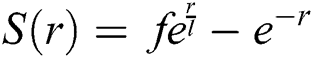
where  is the intensity of attraction, and
  indicates the attractive length scale, This S function computes the factor of attractive and repulsive forces. The distance lies between 0 to 15. The number of repulsions ranged from 0 to 2.079. The comfortable space between the grasshoppers is 2.079 units, meaning that repulsion or attraction is not found when grasshoppers are not in the range of 2.079 units (Comfortable zone). In the case of the simulated grasshoppers, It was found that the difference with the increase in l and f parameters is in social attitude, as shown by Eq. (3). Parameters l and f are evolving independently; their effect on function s is observed.
Attraction, repulsion, and comfortable spaces are changed proportionately concerning parameters I and f., attraction or repulsion spaces regularly to be tiny when using small values such as l = 1.0 or f = 1.0. l = 1.5 and f = 0.5 are selected from the range [7].  component in the next equation is computed as:
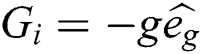
 is gravitational constant,
  is a unity vector toward the centre of the earth. The
  component in Eq. (1) is computed as:
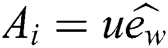
 is Constant drift,
  is a unity vector in the direction of the wind. By substituting all mathematical formulas in Eq. (1) results:
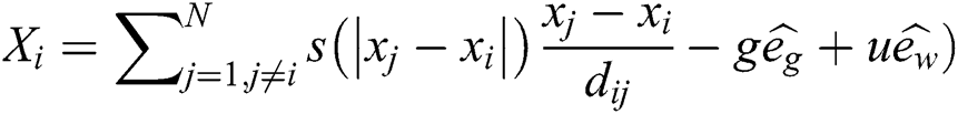
The last equation simulates grasshopper attitude and interaction inside their swarms. In the optimization algorithm, Eq. (6) is not utilized, as it averts the optimization algorithm from exploring and exploiting the search space nearby a solution. This nymph grasshopper model is designed for the grasshopper swarm which resides in the free area. Moreover, this mathematical model was not employed directly to solve optimization problems, as the grasshoppers rapidly achieve the comfort zone, and the swarm does not converge to a specified point. A modified version of Eq. (6) is employed to solve optimization problems:
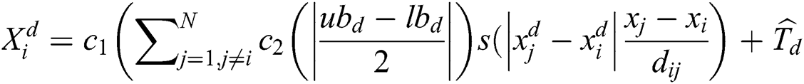
 : Represents the upper and lower bounds,
  : The target value and best solution,
  : coefficients used to shrink the rest zone, repulsion zone, and attraction zone. The gravity component is not utilized, and it’s assumed that wind direction is always toward a target
  . The goal location and current position concerning all other grasshoppers are used to determine the next position of the grasshopper. The parameter
  is used for reducing the movements of grasshoppers around the target, which means that parameter
  is used to balance the exploration and exploitation of the whole swarm around the target. The parameter
  is used to decrease the space to lead the grasshoppers to find the optimal solution in the search space. Both parameters (
 and
and ) can be considered as a single parameter, and it is modified using this equation:
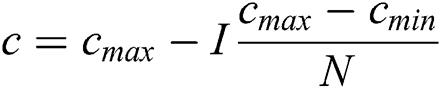
where  : number of current iterations,
  : maximum number of iterations,
  ,
, : The maximum and minimum value of
  .
.
The coefficients appeared two times in the Eq. (7) due to:
• Inactive weight (w) is symbolized by first C. This coefficient is utilized to scale exploration and exploitation of swarm closed to the target. This coefficient is responsible for decreasing the grasshopper movement near the target.
• Minimize the attraction, repulsion, and comfort zone is responsible for the coefficient in the second position.
The simulation is based on the running position of the grasshopper, the target, and the relative location of all other grasshoppers. The first component is the grasshopper location concerning other grasshoppers. Running the position of all grasshoppers, which helps to determine the location of the search agent near the target, is the primary difference between Particle Swarm Optimization (PSO) and Grasshopper Optimization algorithms. PSO is known to be one of the swarm’s attitudes systems, which requires an intelligent collective mindset of bird groups and fish schools (to remain together in communities while going in the same direction). The GOA algorithm uses a single vector as a position, while the PSO uses two vectors: velocity and place for each feature. PSO features do not contribute to the revision of the position of the feature. In a marked difference, the next location of each search agent is decided by all other search agents in GOA.
The term Td imitates grasshopper’s tendency to move in the direction of food. Coefficient c is the deceleration parameter of grasshoppers moving in the direction of food. A random value is multiplied to both parts of the equation for supplying a more random attitude. To obtain random acts in the operation of grasshoppers or their mood in the food search, each variable can be multiplied by arbitrary values.
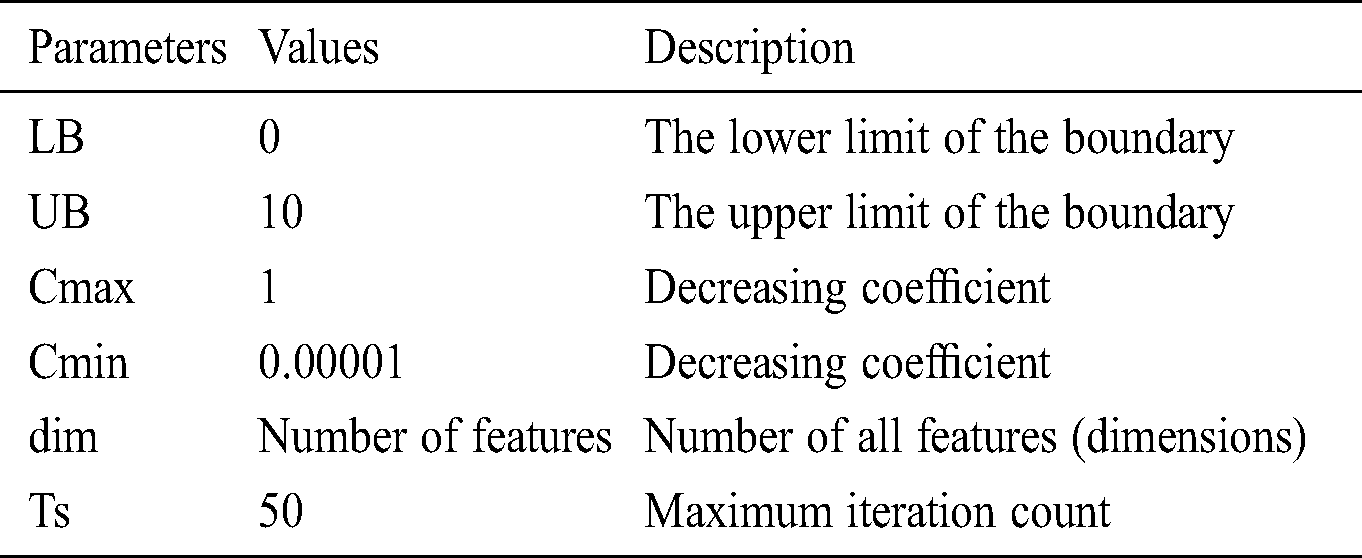
Cmax is C’s maximum value. Cmin is C’s minimum value. I component is the current iteration. The full iteration count is N. In our research, Cmax is loaded as 1, and Cmin is loaded as 0.0001.
The algorithm pseudocode used for feature optimization given below:
Initialize Objective function  no. of dimensions
Generate an initial population of n grasshoppers 
Calculate the fitness of each grasshopper.
T = the best search agent
While stopping criteria not met, do
Update c1 using 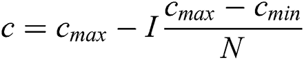
Update c2 using 
for each feature gh in the population do
Normalize the distances between grasshoppers
Update the position of the gh by Eq. (7)
If needed, update the bounds of gh
end
If there is a better solution, update T
Feature optimization is also known as attribute selection in any pattern recognition. It’s like dimensionality reduction; both schemes try to minimize the number of features. However, the main difference is dimensionality reduction creates new combinations of features. On the other hand, feature optimization excludes the features without making any changes [7]. In the next stage, after feature optimization, the optimized features are passed through the fully connected neural network.
A limited number of features are included in feature fusion [8]. By using fusion and optimization, the selected features are taken by neglecting remaining unnecessary features, based on their distinctive characteristics and irrelevance in predicting the outcomes. The fusion of features improves system efficiency by decreasing features and decreasing processing time since fewer features that are used as an input to the artificial neural network have less time to converge and, as a result, improved precision.
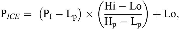
This section characterizes the methods used to distinguish the disease of plant leaves from photographs of plant leaves. The datasets can be accessed from Plant Village’s Master Datasets [9] datasets. Several forms of plant diseases, such as apple, maize, tomato, pipe and pepper, potato, and strawberries, are present in these datasets. The infection types are listed in the figure for each plant group 2. The layout and complete identification and classification model followed the methodology of the plant leaf disease [10] is shown. Improving photos is used to obtain an exact picture of a plant state, and the grey level pictures are identified. The pixel colour values usually are 0 and 255 on the lowest and highest edges. The boundaries of image contrast are specified as ‘Lo’ and ‘Hi’ with the aid of the image contrast enhancement. This normalization uses the image of the planted leaf to find these colour pixel image values, which require the increase in the contrast, namely Lp and Hp.
All pixels ( ) of the plant leaf image is enhanced using this equation:
The extracted characteristics of the fragmented image are highlighted, as shown in Fig. 1, by running the SURF system as a feature extraction method [11] for extracting only the area of the leaf affected by the disease.
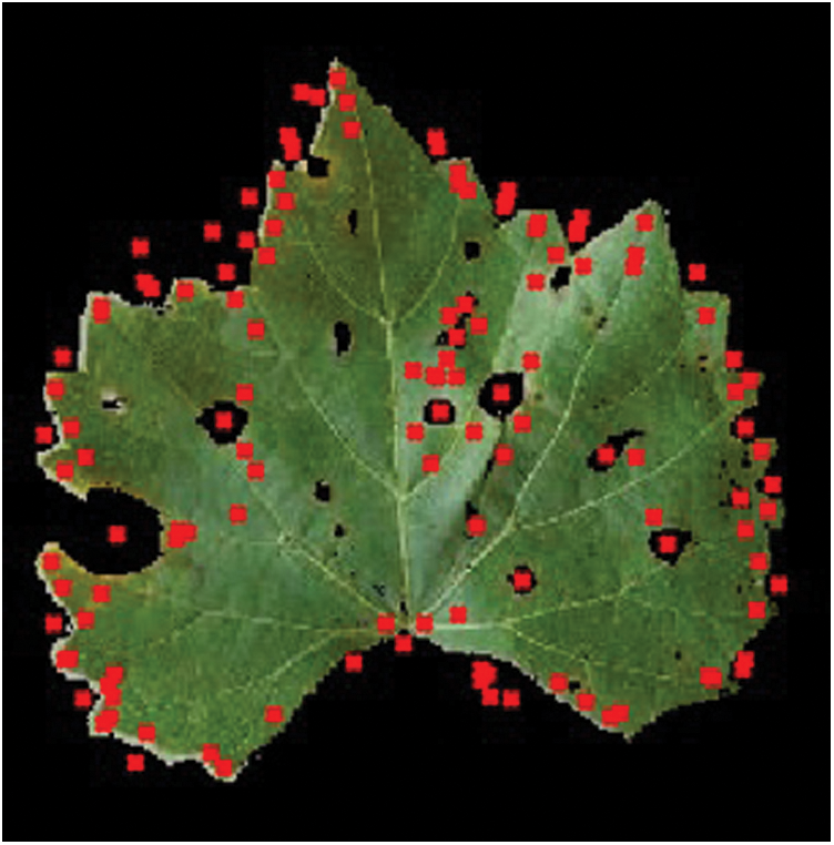
Figure 1: Extracted SURF features after segmentation
3.3 Fused-Modified Grasshopper Optimization Algorithm
It initializes the grasshopper’s position in space. Each grasshopper’s position is set to 1.
3.3.2 Fitness Function and Fusion
FMGOA is used to optimize SURF features and to remove the unwanted feature sets by using the different objective fitness function with similarity measure to choose the distinctive optimized features only.

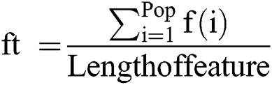
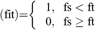
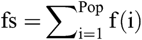
Fitness function:
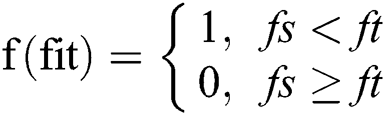

The fittest fused function after calculation of each agent’s fitness to select the most qualified and distinctive features for final optimization using the fitness and sigmoid similarity equations, any two features that have high similarity measure is utilized into one feature and applied for all f(fit) features and then returns the fitness value of each grasshopper. The mathematical properties of sigmoid similarity are presented as follows [12].
1. Boundaries: 
2. Maximum similarity:
if  , then
  , since
  and
and  and the function
  tends to 1 when
  tends to infinity.
3. Commutativity: 
4. Monotonicity:
If  and
and  , then
  .
.
If  and
and  , then
  .
.
The outputs of sigmoid similarity will belong to a range of 0 and 1, and maximum output is gained when the compared features are not distinctive, any features that have sigmoid similarity is fused to be one feature. The ultimate goal is to minimize the importance of this fitness function to find a better solution for the identification of plant diseases. Presented Fused Modified Grasshopper Optimization Algorithm (FMGOA) processes feature set as input and output as a reduced feature set that upgrades system performance. The FMGOA pseudocode is listed in the following section, and the input parameters are shown in Tab. 1. The modulated algorithm pseudocode used for feature optimization given below:
Input: SURF Key points as a feature vector
Output: Optimized feature points
Initialize GOA parameters
Iterations (I)
Number of Population (Pop)
Lower Bound (LB)
Upper Bound (UB)
Fitness function
Number of Selection (Ns)
Calculate Ts = Size (SURF Keypoints)
Define fitness function of GOA:
Fitness function:
For i = 1 → Ts

 = fitness function which defines by Eq. (14)
No. of variables = 1
Opt_value = GOA (P, Iterations, LB, UB, Ns, f(fit))
End
While Ts ~ = Maximum
Fused_features_based_on_sigmoid_similarity
If needed, update the bounds of grasshoppers.
End
Optimized data = Opt_value
Apply ANN and SVM on the positions of agents
Return the classification accuracy from the selected features
Use confusion matrix to calculate accuracy percentage, precision, recall, f-measure, and error rate.
The presented algorithm used to detect diseases of plant leaves has been modified to boost efficiency.
This section describes the necessary experiment setup, input parameters, ML algorithms, optimized parameters, and all data sets.
The Intel ® 2.7 GHz dual-core Core i5 processor (Turbo Boost up to 3.1 GHz) system configuration under macOS 10.15.4 (version) was used to test the proposed algorithm. It was implemented using Matlab R2019 9.6 (version).
a) Support Vector Machines
Support Vector machines is a linear supervised learning classifier usually utilized for classification applications, which includes interpretation of labelled features in the given training dataset and predication of unlabelled features in the test dataset [6]. In SVM, a feature pixel is viewed as an R-dimensional vector and is required to know whether such points can be separated with an R-1-dimensional hyperplane. Multiclass SVM aims to determine labels to images, where the labels are drawn from a finite set of several images. The final approach for doing so is to reduce the single multiclass classification into multiple binary classifications.
b) Artificial Neural Network
Feature optimization is also called function selection or attribute in any pattern detection or recognition software. Feature optimization differs from dimensionality reduction techniques, but both methods aim at reducing the number of features in feature sets. The dimensionality reduction approach creates new function combinations while function optimization approaches use features present in function sets and delete them without changing them. Before feature optimization, the optimized function is used as a collection of ANN [13] inputs to train the proposed methodology; the fusion and optimization of extracted features minimize the number of inputs. The ANN pseudocode is the following:
Input: Optimized feature points as a Training Data (TD),
Target as a diseases types (TR) and Neurons (Ne)
Output: Classify leaf disease
Initialize ANN with parameters
No. of Epochs/Iterations (E)
Neurons as the carrier (Ne)
Training parameters for performance evaluation: Cross-Entropy, Gradient, Mutation, and Validation
Training used the technique: Scaled Conjugate Gradient (Training)
TD Division: Random
For each set of T
If Training Data (TD)  1st Category of feature set

Else if Training Data (TD)  2nd Category of feature set

Else if Training Data (TD)  3rd Category of feature set

Else if Training Data (TD)  4th Category of feature set

End
Initialized the ANN in the system using Training data (TD) and their Target (TR)
Net = patternnet ( ) // here DNN is initialized and stored in the net as a structure
Set the training parameters according to the requirements and train the system
Net = Train (Net, TD, Group)
Classification Results = simulate (Net, Test leaf ROI optimized feature)
If Classification Results = True
Show classified results in terms of the leaf disease
Calculate the performance parameters
End
Returns: Classified Results
End
c) Fusion of classifiers
Early fusion has some advantages over late fusion strategies, given that they are conducted through the training sets properly [14]. Various feature training sets show different characteristics of the same pattern and combining those features retain active discriminant information while altogether remove the redundant data. In our approach, we have fusion that separates the training datasets into two segments; each segment is passed through training and then exceeded the classification. In contrary to early fusion, late fusion approaches train separate classifiers for each of the image channels present in our dataset. If we have  different classifiers, then it yields various learning modalities. After that, late fusion approaches merge those
  different classifier results into one classification value [15]. Late fusion approaches have several obvious obstacles compared to early fusion approaches. First of all, the late fusion approach increases the computational time required due to the higher number of classifiers to be trained. The second obstacle is those classifier models are not symbolized with information from different models, so correlations between those models are not considered in the classifier outputs [16]. Despite these apparent drawbacks, late fusion approaches are stated to acquire comparable or even better results to early fusion approaches in some applications. Yang et al. refer to this to heterogeneous and independent nature of multimedia features as hierarchical regression for multimedia analysis [16]. The late fusion function contains the function that combines the prediction outputs of both methodologies, the Fused Optimized Artificial Neural Network (FOANN) and Fused Optimized Support Vector Machine (FOSVM) which outcomes by taking the arithmetic mean of them as a fusion method [16].
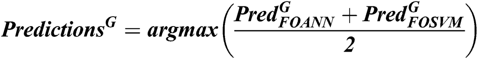
where 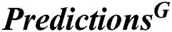 is the prediction of fusion classifiers of FOANN and FOSVM classification result, classification result
  is the prediction of classification of using fused optimized artificial neural networks classifier,
  is the prediction of classification of using a fused optimized SVM classifier.
The datasets form part of the public datasets of plant villages containing different categories of plant leaves with many types of plant diseases, and seven categories are used for the assessment of the technique, i.e., apples; corn; grapes; peaches; peppers; potatoes; and strawberries as shown in Fig. 2.
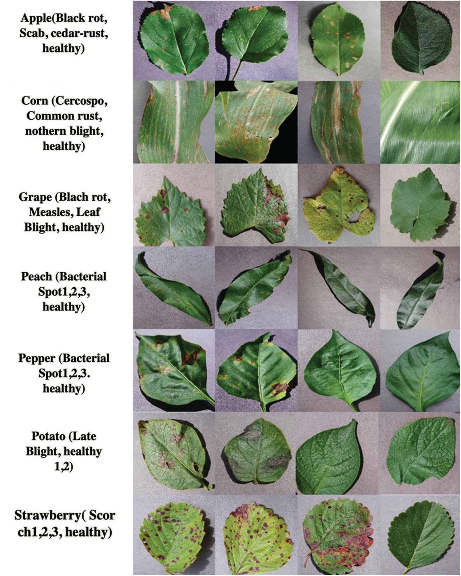
Figure 2: Categories of plant leaves
The findings and a comparative analysis are seen in this section following the review of the paper. Model parameters, such as precision, alert, f-measurement, error and precision, are determined for the evaluation [17,18]. The dataset consists of over twenty thousand images of seven types, 14 infection classes and 7 safe form classes. The initial analysis is conducted using fusion and optimization. The product of optimization and fusion of the effects of accuracy classifiers; each value is an average of 10 accuracy values, shown in Tab. 2.
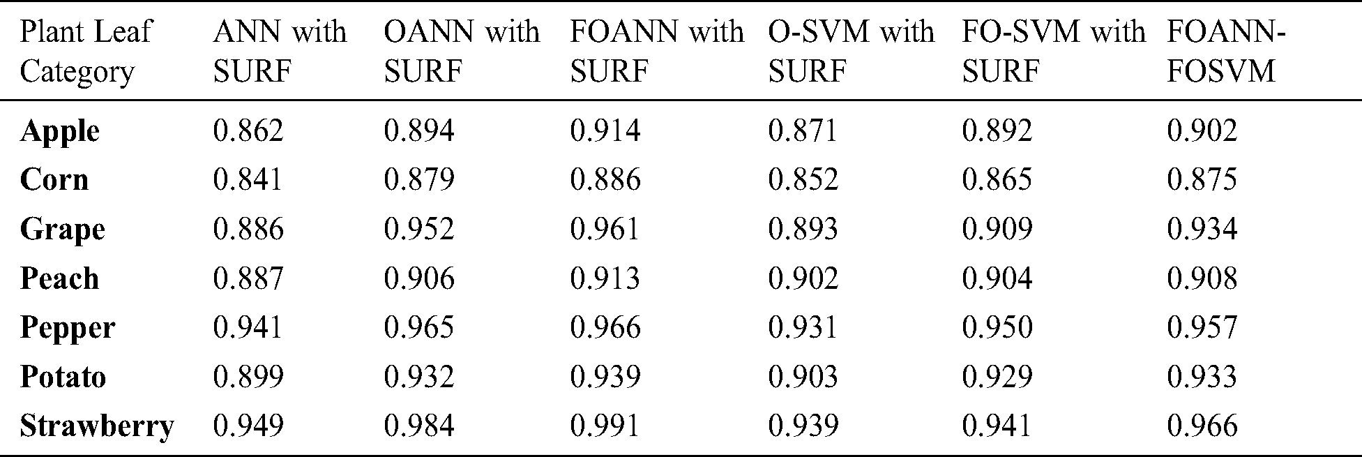
Fig. 3 and Tab. 2 demonstrates the accurate estimation of the methodologies approach. The figure reflects the contrast between the Fused optimized artificial neural network FOANN and the SVM classifier. Precision is the mean of the right values for the total data set in the assessment process. We use seven types of plants with an Optimized ANN model using SVM fusion, the best result of which is 0.991 strawberry. The best outcome for corn is FOANN-SURF with 0.886. The best result for grapes is FOANN-SURF with 0.961. It is FOANN-SURF with 0.913 for Peach. With 0.966 for Pepper. With 0.939 for Potato. Approximately 2.237 percent improvement in precision results for apple plant leaves by using FOANN compared to our previous OANN model. The use of ANN-SURF also has the lowest precision performance.
Figure 3: Precision results chart
Fig. 4 and Tab. 3 displays the methodologies approach for recall estimation. This figure shows a contrast between FOANN and SVM classifiers, the optimized fused neural network. The recall rate is the total number of actual samples that are correctly treated during the classification process. The best outcome is strawberry with 0,959 using the total number of samples from the same categories in training data using seven plant types with an optimized ANN model based on SVM fusion. FOANN-SURF with 0.834 is the best result for maize. FOANN-SURF with 0.901 is the best result for grapes. FOSVM-SURF is 0.89 for Peach. For Peach. And 0.956 for Pepper. With 0.941 for Potato. The accuracy of apple plant leaves when using FOANN has increased around 3,846 percent compared with our previous OANN model. The use of ANN-SURF also results in the lowest retrieval.
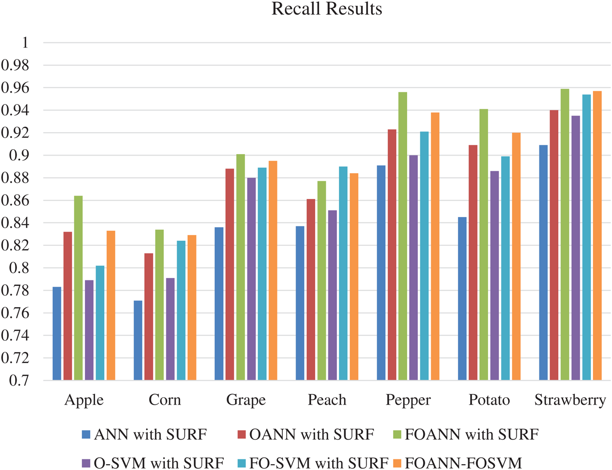
Figure 4: Recall results
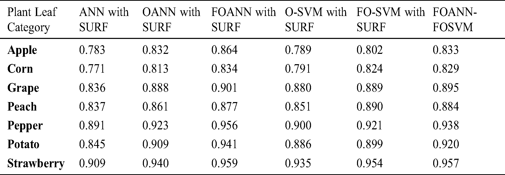
Fig. 5 and Tab. 4 demonstrates the technique approach reliable measurement. The figure shows the contrast between the FOANN and SVM classification optimized artificial neural networks. F-measure is the harmonic average accurate and reminder rate. We use seven plant forms; the best result is 0.975 strawberry with fusion-optimized ANN models and the fusion of SVM. FOANN-SURF with 0.859 is the best result for maize. The best result for grapes is 0.930 FOANN-SURF. FOANN-SURF is 0.896 for Peach. For Peach. With 0.961 for Pepper. With 0.94 for Potato. The use of ANN- SURF also results in the lowest f-measure.
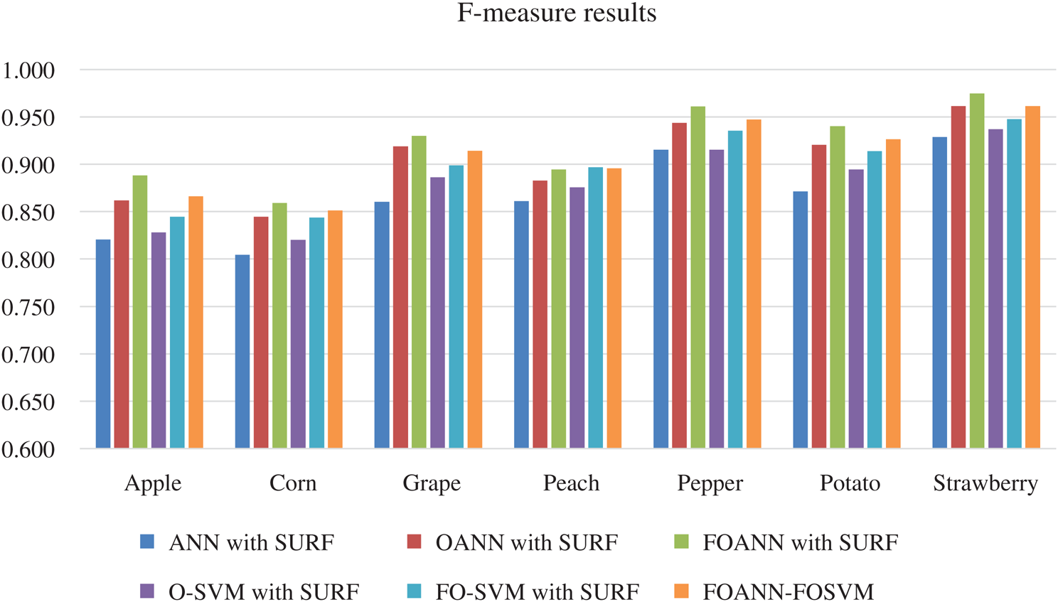
Figure 5: F-measure results
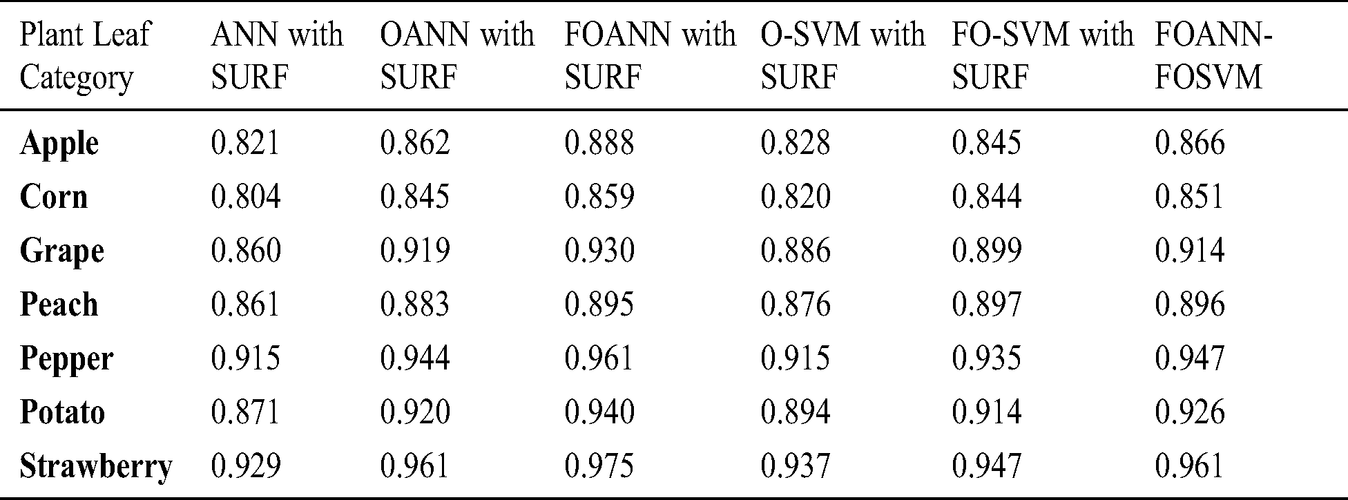
Fig. 6 and Tab. 5 illustrates the technique approach error estimation. The figure indicates a contrast between FOANN and FOSVM classifications of the Fused optimized artificial neural network, with the lowest FOANN-SURF error rate at 0.08. FOANN-SURF with 0.62 is the lowest error rate for corn.
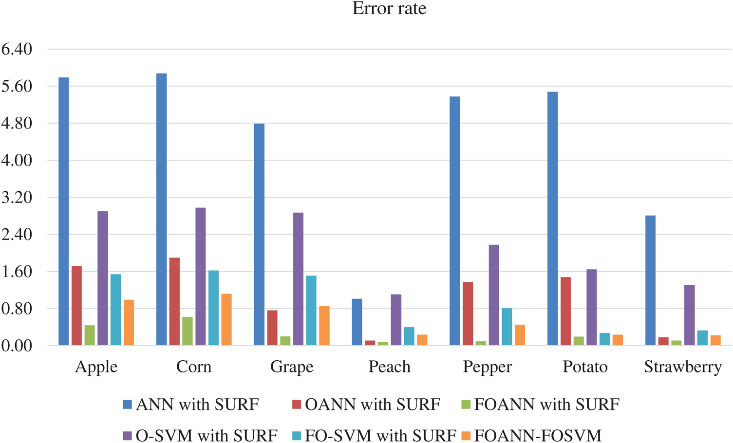
Figure 6: Error results
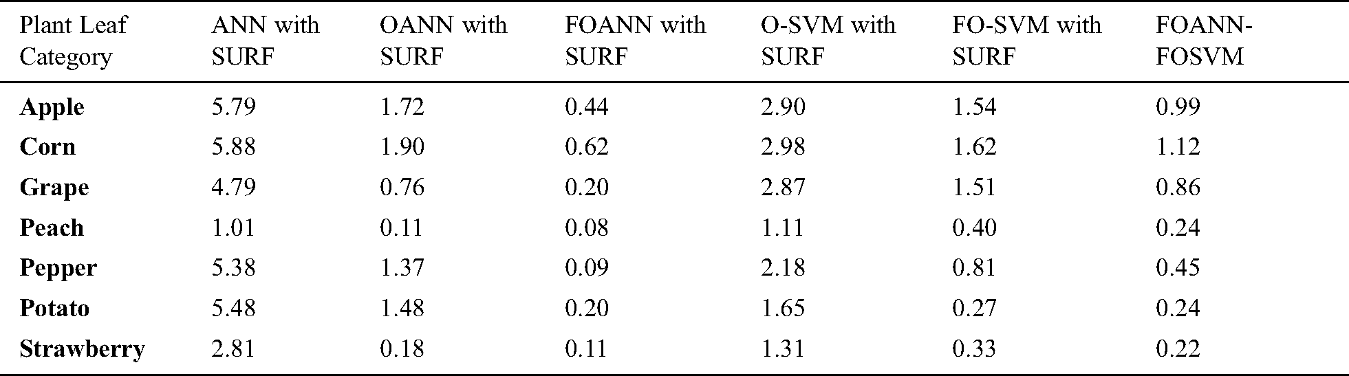
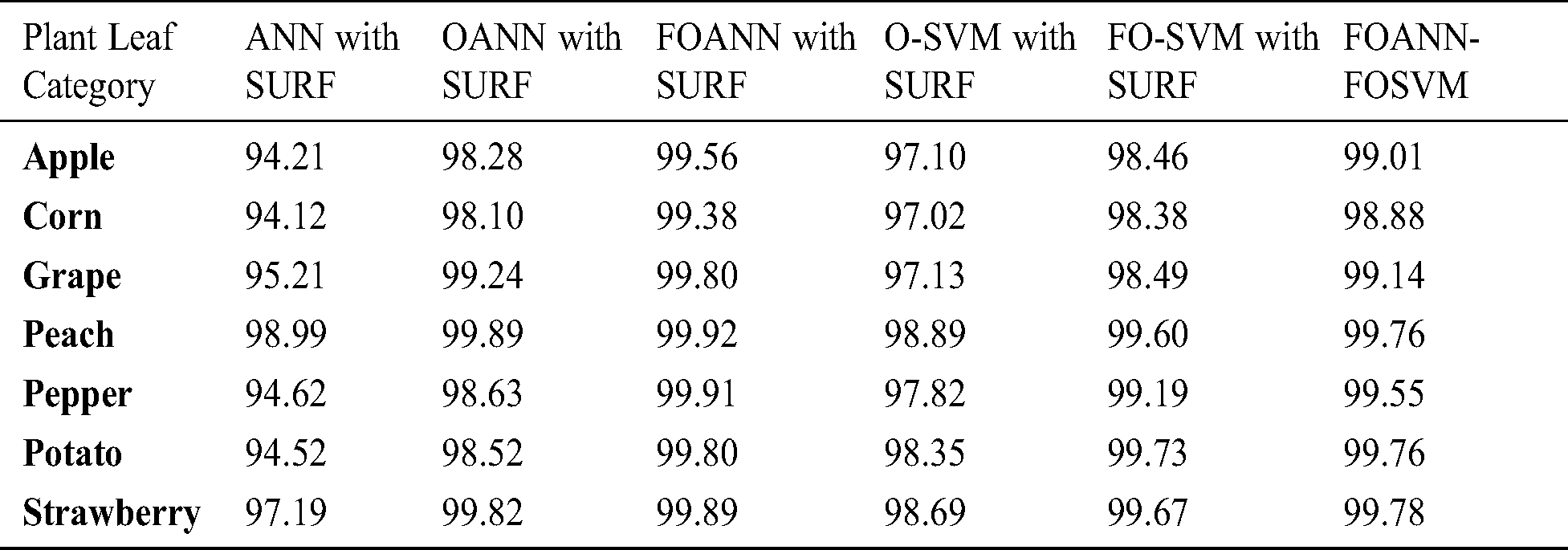
Fig. 7 and Tab. 6 show a calculation of the accuracy of the approach proposed. The designed system is primarily concerned with accuracy improvement and avoids overfitting and underfitting issues. The best result is FOANN-SURF 99.92% with peach plant leaves. In the figure, the Optimized ANN models are compared to FOSVM. The x-axis indicates the samples, while the Y-axis represents accuracy values. Approximately 2.1% improvement of the proposed model concerning our fused optimized ANN models in accuracy relative to and roughly our previously optimized ANN. 4.31% improvement from machine learning models yet available.
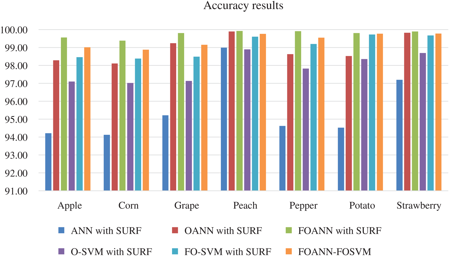
Figure 7: Accuracy results
6 Conclusion: Comparison Between FMGOA and MGOA
In this article, a novel experimental study of multiple classifiers is performed. The identification of plant disease in the early stage is mandatory for researchers because of agricultural issues to identify diseases and other epidemics. Many models are designed to use their leaf pixel properties to find the best fusion for plant identification [19]. The proposed methodology has been executed in various procedures; reducing features have improved the performance and computational time due to lower features have been used as an input to the artificial neural network and thus shorter computational time. The accuracy of the proposed work for plant identification has been improved and improved using the multiple fusion of classifiers. It is concluded from the results of the experiments that the accuracy of the proposed model (FMGOA). With FOANN as fused-optimized Artificial Neural Network increases by approximately 2.1% more than our previous modified technique, Modified Grasshoppers Optimization Algorithm (MGOA) without fusion in our last article “Evolutionary Feature Optimization for Plant Leaf Disease Detection by Deep Neural Networks,” accurate Classification and better by 5.6% than ANN with SURF, the accuracy results in ANN with SURF have the lowest accuracy results. These findings are more reliable than in recent studies [20–26]. Other methodologies could be fused and tested, and our framework will try methods in different fields and environments that aim to establish a useful automated model for identification based on the complex set of classifications.
Acknowledgement: The authors would like to thank the anonymous reviewers for their valuable comments and suggestions to improve the quality of the article.
Funding Statement: The authors received no specific funding for this study.
Conflicts of Interest: The authors declare that they have no conflicts of interest to report regarding the present study.
1. B. M. Yahya and D. Z. Seker. (2019). “Designing weather forecasting model using computational intelligence tools,” Applied Artificial Intelligence, vol. 33, no. 2, pp. 137–151. [Google Scholar]
2. Z. Chuanlei, Z. Shanwen, Y. Jucheng, S. Yancui and C. Jia. (2017). “Apple leaf disease identification using the genetic algorithm and correlation-based feature selection method,” International Journal of Agricultural and Biological Engineering, vol. 10, no. 2, pp. 74–83. [Google Scholar]
3. A. Nayyar, S. Garg, D. Gupta and A. Khanna. (2018). “Evolutionary computation theory and algorithms,” in A. Nayyar, D.- N. Le and N. G. Nguyen (eds.Advances in Swarm Intelligence for Optimizing Problems in Computer Science, 1st ed., Chapter 1Boca Raton, FL, USA: CRC Press, pp. 1–26. [Google Scholar]
4. S. Saremi, S. Mirjalili and A. Lewis. (2017). “Grasshopper optimization algorithm: Theory and application,” Advances in Engineering Software, vol. 105, pp. 30–47. [Google Scholar]
5. P. Tumuluru and B. Ravi. (2018). “Chronological grasshopper optimization algorithm-based gene selection and cancer classification,” Journal of Advanced Research in Dynamical and Control Systems, vol. 10, no. 3, pp. 80–94. [Google Scholar]
6. H. T. Ibrahim, W. J. Mazher, O. N. Ucan and O. Bayat. (2019). “A grasshopper optimizer approach for feature selection and optimizing SVM parameters utilizing real biomedical data sets,” Neural Computing and Applications, vol. 31, no. 10, pp. 5965–5974. [Google Scholar]
7. S. Shahrzad, S. Mirjalili, Se Mirjalili and J. S. Dong. (2019). “Grasshopper optimization algorithm: Theory, literature review, and application in hand posture estimation,” Nature-Inspired Optimizers, Studies in Computational Intelligence, vol. 811, pp. 107–122. [Google Scholar]
8. S. Zheng, P. Qi, S. Chen and X. Yang. (2019). “Fusion methods for CNN-based automatic modulation classification,” IEEE Access, vol. 7, pp. 66496–66504. [Google Scholar]
9. A. Camargo and J. S. Smith. (2009). “An image-processing based algorithm to automatically identify plant disease visual symptoms,” Biosystems Engineering, vol. 102, no. 1, pp. 9–21. [Google Scholar]
10. V. Pooja, R. Das and V. Kanchana. (2017). “Identification of plant leaf diseases using image processing techniques,” in IEEE Technological Innovations in ICT for Agriculture and Rural Development, Chennai, India, pp. 130–133. [Google Scholar]
11. H. Bay, T. Tuytelaars and L. V. Gool. (2006). “Surf: Speeded up robust features,” in Computer Vision–ECCV, Heidelberg, Berlin, Germany: Springer, vol. 3951, pp. 404–417. [Google Scholar]
12. S. Likavec, I. Lombardi and F. Cena. (2019). “Sigmoid similarity-A new feature-based similarity measure,” Informatics Sciences, vol. 481, pp. 203–218. [Google Scholar]
13. K. Golhani, S. K. Balasundram, G. Vadamalai and B. Pradhan. (2018). “A review of neural networks in plant disease detection using hyperspectral data,” Information Processing in Agriculture, vol. 5, no. 3, pp. 354–371. [Google Scholar]
14. A. Roitberg, T. Pollert, M. Haurilet, M. Martin and R. Stiefelhagen. (2019). “Analysis of deep fusion strategies for multi-modal gesture recognition,” in IEEE Conf. on Computer Vision and Pattern Recognition (CVPR) Workshops, Long Beach, CA, USA, pp. 198–206. [Google Scholar]
15. H. Ergun, Y. C. Akyuz, M. Sert and J. Liu. (2016). “Early and late level fusion of deep convolutional neural networks for visual concept recognition,” International Journal of Semantic Computing, vol. 10, no. 3, pp. 379–397. [Google Scholar]
16. J. M. Preez-Rua, V. Vielzeuf, S. Pateux, M. Baccouche and F. Jurie. (2019). “MFAS: Multimodal fusion architecture search,” in IEEE, California, USA. [Google Scholar]
17. J. G. A. Barbedo. (2016). “A review on the main challenges in automatic plant disease identification based on visible range images,” Biosystems Engineering, vol. 144, pp. 52–60. [Google Scholar]
18. I. F. Salazar-Reque, S. G. Huamán, G. Kemper, J. Telles and D. Diaz. (2019). “An algorithm for plant disease visual symptom detection in digital images based on superpixels,” International Journal on Advanced Science, Engineering and Information Technology, vol. 9, no. 1, pp. 194–203. [Google Scholar]
19. V. Vielzeuf, A. Lechervy, S. Pateux and F. Jurie. (2019). “CentralNet: A multilayer approach for multimodal fusion,” in European Conf. on Computer Vision Workshops: Multimodal Learning and Applications, Munich, Germany, vol. 11134, pp. 575–589. [Google Scholar]
20. L. G. Nachtigall, R. M. Araujo and G. R. Nachtigall. (2016). “Classification of apple tree disorders using convolutional neural networks,” in IEEE 28th Int. Conf. on Tools with Artificial Intelligence, San Jose, CA, USA, pp. 472–476. [Google Scholar]
21. B. Liu, Y. Zhang, D. J. He and Y. Li. (2017). “Identification of apple leaf diseases based on deep convolutional neural networks,” Symmetry, vol. 10, no. 1, pp. 11. [Google Scholar]
22. V. Singh and A. K. Misra. (2017). “Detection of plant leaf diseases using image segmentation and soft computing techniques,” Information Processing in Agriculture, vol. 4, no. 1, pp. 41–49. [Google Scholar]
23. S. Kaur, S. Pandey and S. Goel. (2019). “Plants disease identification and classification through leaf images: A survey,” Archives of Computational Methods in Engineering, vol. 26, no. 2, pp. 507–530. [Google Scholar]
24. S. Kalaivani, S. P. Shantharajah and T. Padma. (2019). “Agricultural leaf blight disease segmentation using indices based histogram intensity segmentation approach,” Multimedia Tools and Applications, vol. 79, no. 2, pp. 1–15. [Google Scholar]
25. S. S. Chouhan, U. P. Singh and S. Jain. (2020). “Applications of computer vision in plant pathology: A survey,” Archives of Computational Methods in Engineering, vol. 27, pp. 611–632. [Google Scholar]
26. S. Zhang, Z. You and X. Wu. (2019). “Plant disease leaf image segmentation based on superpixel clustering and EM algorithm,” Neural Computing and Applications, vol. 31, no. 2, pp. 1225–1232. [Google Scholar]
 | This work is licensed under a Creative Commons Attribution 4.0 International License, which permits unrestricted use, distribution, and reproduction in any medium, provided the original work is properly cited. |