Computers, Materials & Continua DOI:10.32604/cmc.2021.012301
Article

Optimal Control Model for the Transmission of Novel COVID-19

Isa Abdullahi Baba1,*, Bashir Ahmad Nasidi1 and Dumitru Baleanu2,3,4

1Department of Mathematical Sciences, Bayero University Kano, Nigeria
2Department of Mathematics, Cankaya University, Ankara, 06530, Turkey
3Institute of Space Sciences, Bucharest, Romania
4Department of Medical Research, China Medical University Hospital, Taichung, Taiwan
*Corresponding Author: Isa Abdullahi Baba. Email: iababa.mth@buk.edu.ng
Received: 24 June 2020; Accepted: 06 October 2020

Abstract: As the corona virus (COVID-19) pandemic ravages socio-economic activities in addition to devastating infectious and fatal consequences, optimal control strategy is an effective measure that neutralizes the scourge to its lowest ebb. In this paper, we present a mathematical model for the dynamics of COVID-19, and then we added an optimal control function to the model in order to effectively control the outbreak. We incorporate three main control efforts (isolation, quarantine and hospitalization) into the model aimed at controlling the spread of the pandemic. These efforts are further subdivided into five functions; u1(t) (isolation of the susceptible communities), u2(t) (contact track measure by which susceptible individuals with contact history are quarantined), u3(t) (contact track measure by which infected individualsare quarantined), u4(t) (control effort of hospitalizing the infected I1) and u5(t) (control effort of hospitalizing the infected I2). We establish the existence of the optimal control and also its characterization by applying Pontryaging maximum principle. The disease free equilibrium solution (DFE) is found to be locally asymptotically stable and subsequently we used it to obtain the key parameter; basic reproduction number. We constructed Lyapunov function to which global stability of the solutions is established. Numerical simulations show how adopting the available control measures optimally, will drastically reduce the infectious populations.

Keywords: COVID-19; optimal control; Pontryaging maximum principle; mathematical model; existence of control; stability analysis

1  Introduction

The novel coronavirus pneumonia which was officially named as Corona Virus Disease 2019 (COVID-19) by World Health Organization (WHO) was reported first in late December 2019, in Wuhan, China [1]. The source of the virus is not yet known, but genetic investigation revealed that COVID-19 virus has the same genetic characteristics with SARS-CoV2 (which was likely to be originated from bats) [2]. It is also found to be significantly less severe than the other two coronaviruses; Severe Acute Respiratory Syndrome (SARS-COV) and Middle East Respiratory Syndrome (MERS-COV) that caused an outbreak in 2002 and 2008 respectively [3]. The most important routes of human to human transmission of COVID-19 are respiratory droplets and contact transmission [4]. After the incubation period which is generally 2–14 days, the mild symptoms may persist from high degree fever, cough and shortness of breath to being severely ill and subsequently death [4].

As scientists all over the world are busy trying to develop a cure and vaccine, all hands must be put together to support and comply with the standard recommendations that can lower the transmissions of the disease. This is why, the following measures must be taken; social distancing, self-isolation, use of personal protective equipment (such as face mask, hand globes, overall gown, etc.), regular hand washing using soap or sanitizer, avoid having contact with person showing the symptoms and report any suspected case. Moreover, relevant authorities must engage in widely public orientation exercise for sensitization and enlightenment, banning of social (or religious) gathering and local (or international) trip, contact tracing and isolation of infected individuals, providing sanitizers at public domains like markets and car parks, fumigating exercise, and to the large extent imposing lockdown.

The scourge does not only cause apocalyptic proportion in terms of infection, morbidity and fatality, but also socio-economic consequences. To control the above mentioned problems, there is need to have better understanding on the transmission dynamics of the disease. This could be achieved by developing mathematical model that optimizes the possible control measures.

Optimal control is considered as an effective mathematical tool used to optimize the control problems arising in different field including epidemiology, aeronautic engineering, economics, finance, robotics, etc [5]. Mathematical model offers an insight in to the transmission and control of infectious disease [6–13]. Zhao et al. [14] developed a Susceptible, Un-quarantined infected, Quarantined infected, Confirmed infected (SUQC) model to characterize the dynamics of COVID-19 and explicitly parameterize the intervention effects of control measures. Song et al. [15] established deterministic mathematical model (SEIHR) to suit Korean outbreak, in which he estimated the reproduction number and the effect of preventive measures.

Tahir et al. [16] developed a mathematical model (for MERS) in form of nonlinear system of differential equations, in which he considered a camel to be the source of the infection. The virus is then spread to human population, then human to human transmission, then human to clinic center and then human to care center. They used Lyapunov function to investigate the global stability analyses of the equilibrium solutions and subsequently obtained the basic reproduction number or roughly, a key parameter describing transmission of the infection.

Yang et al. [17] proposed a mathematical model to investigate the current outbreak of the coronavirus disease (COVID-19) in Wuhan, China. The model described the multiple transmission pathways in the infection dynamics, and emphasized the role of environmental reservoir in the transmission and spread of the disease. However, the model employed non-constant transmission rates which change with the epidemiological status and environmental conditions and which reflect the impact of the ongoing disease control measures.

Chen et al. [18] modeled (based on SEIR) the outbreak in Wuhan with individual reaction and governmental action (holiday extension, city lockdown, hospitalization and quarantine) in which they estimated the preliminary magnitude of different effect of individual reaction and governmental action. Sunhwa et al. [19] developed a Bats-Hosts-Reservoir-People (BHRP) transmission network model for the potential transmission from the infection source (probably bats) to the human, which focuses on calculating R0. Elhia et al. [20] developed a mathematical model based on the epidemiology of COVID-19, incorporating the isolation of healthy people, confirmed cases and close contacts.

Most of these models have a general shortcoming of not taking into consideration time dependent control strategies. For the model to be more realistic, it has to be time dependent [21–26]. Here, we modified the work of Elhia et al. [20], by incorporating control functions with the aim of deriving optimal control that drastically minimizes the spread of the infection.

The paper is arranged in the following order: Chapter 1 gives the introduction, Chapter 2 gives preliminary definitions and theorems, Chapter 3 is the model formulation, Chapter 4 discusses the formulation and analysis of optimal control, Chapter 5 presents local and global stability analyses of the solutions of the model and the derivation of the reproduction number and lastly Chapter 6 gives numerical simulation results and then the discussion follows.

2  Preliminary Definitions and Theorem

Definition 1 (Optimal Control) [27]: A fairly general continuous time optimal control problem can be defined as follows:

Problem i: To find the control vector trajectory that minimizes the performance index:

Subject to:

where , and is a terminal cost function.

Problem ii: Find tf and to minimize:

Subject to:

This special type of optimal control problem is called the minimum time problem.

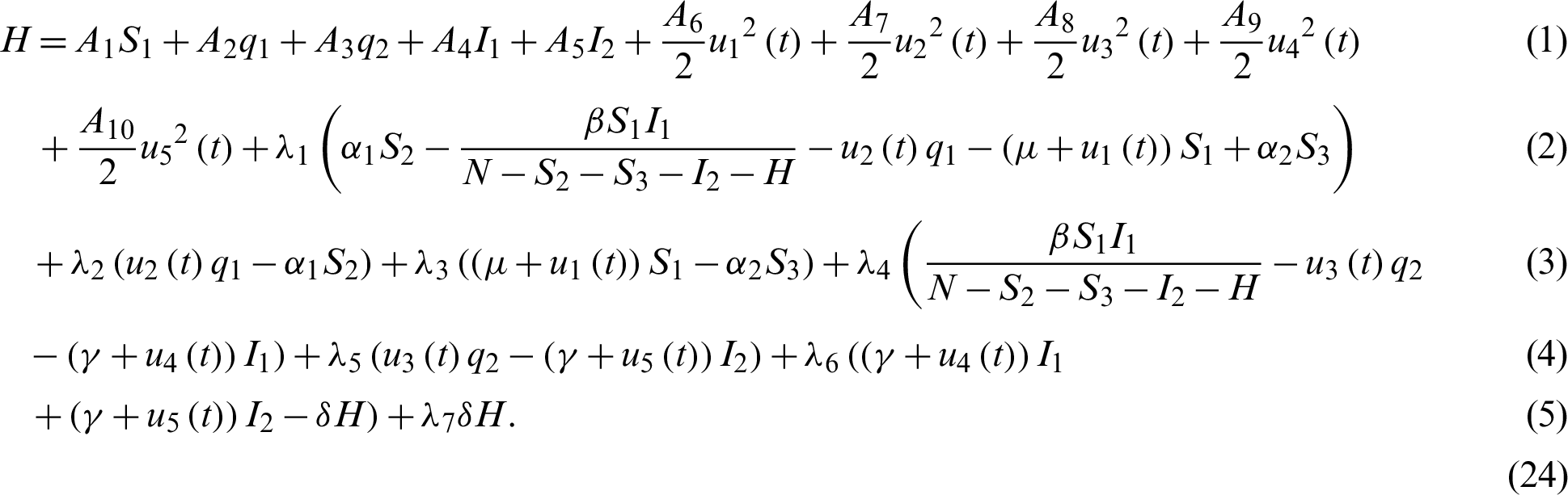
Definition 2 (Hamiltonian): A time varying Lagrange’s multiplier function , also known as the co-state define Hamiltonian function H as:

such that

Theorem 1 (Pontryagin Maximum Principle): If is a solution of the optimal control problem Eqs. (1) and (2) then there exists a non-zero absolutely continuous function such that satisfy the system

such that, for almost all the function in Eq. (3) attains its maximum:

and such that at terminal time tf the conditions

If the functions satisfy the relation Eqs. (5) and (6) (i.e., are Portryagin extremals), then the condition

Remark 1: Becerra states that for a minimum, it is necessary for the stationary (optimality) condition to give:

3  Model Formulation

We know that most people are susceptible to COVID-19 and the patients in the incubation period can infect healthy people. We denote the population of susceptible people with S, the patients in the incubation period and the patients that are yet to be diagnosed by I, patients in the hospital by H, removed people by R, respectively. Here the infectivity of the patients in the incubation period and the patients that are yet to be diagnosed are assumed to be the same.

After the outbreak of COVID-19, susceptible people are advised to lock themselves down at home, and all close contacts of infected individuals tracked are quarantined. Therefore, we divide the population of susceptible people into; susceptible people (S1), the quarantined susceptible people (by close contacts tracked measure) (S2) and general isolated susceptible people (due to community lockdown) (S3). Infected people population is divided into general infected people, including the patients in the incubation period and the infected people that are yet to be diagnosed (I1) and infected people that are quarantined (I2). Here we assume that all susceptible people isolated at home cannot be infected and all infected people isolated at home cannot infect healthy people. Thus, we establish the transmission dynamics of the disease as in Fig. 1.

Figure 1: Transmission dynamics of the disease

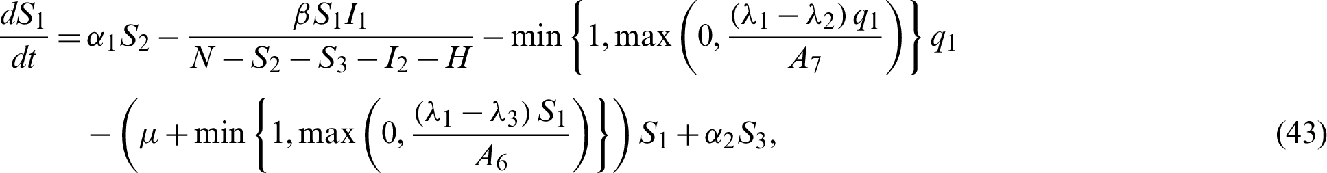
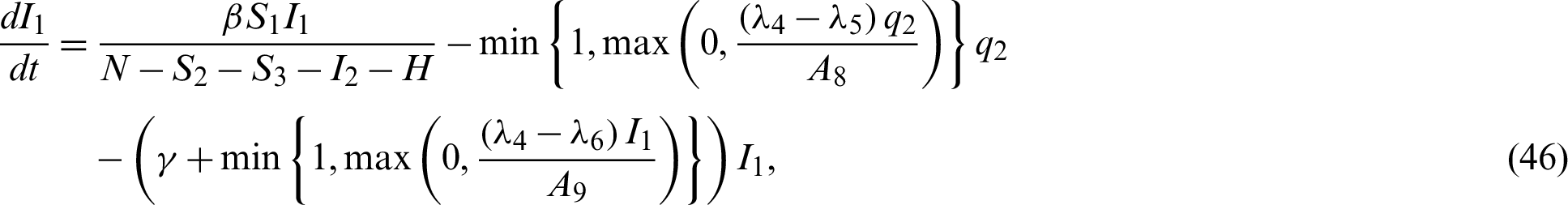
The transmission dynamics can be described by the nonlinear system of first order differential equations as follows:

where,

When patients go to hospital and are diagnosed (I1 +I2), by the close contacts tracked measure, susceptible people (q1) and infected people (q2) are quarantined by the proposition b. Here the number of quarantined susceptible people (q1) and quarantined infected people (q2) are less than the number of susceptible people (S1) and infected people (I1) respectively. Then 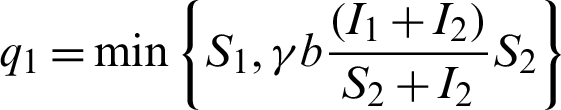and .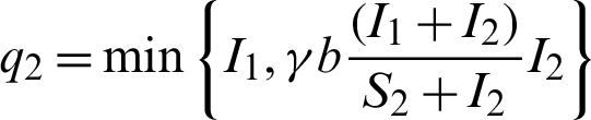

After the isolation of 14 days , the quarantined susceptible individuals become susceptible. When quarantined infected people have symptoms, they are hospitalized and diagnosed (I2). After the time of treatment , they are removed from the hospital. The communities are isolated and healthy people are also advised to isolate themselves at home unless they have something urgent to deal with. Then and denote the weak movements of population from susceptible to isolated susceptible and from isolated susceptible to susceptible, respectively.

4  Optimal Control

Here the detail formulation and analysis of the optimal control problem with respect to the model Eqs. (8)–(14) is given.

4.1 Formation of an Optimal Control

The aim of the control strategy is to prevent the susceptible population from becoming infected and reduce the infected population by increasing hospitalization which eventually reduces the number of new cases.

Let the control functions

be the rate at which susceptible communities are isolated.

be the contact track measure by which susceptible individuals with contact history are quarantined.

be the contact track measure by which infected individuals are quarantined.

be the control effort of hospitalizing the infected I1.

be the control effort of hospitalizing the infected I2.

The dynamics of control system can be described by the following system of nonlinear ODE;

For a fixed terminal time tf, the problem to minimize the objective functional associated to system Eq. (15) through Eq. (21) is

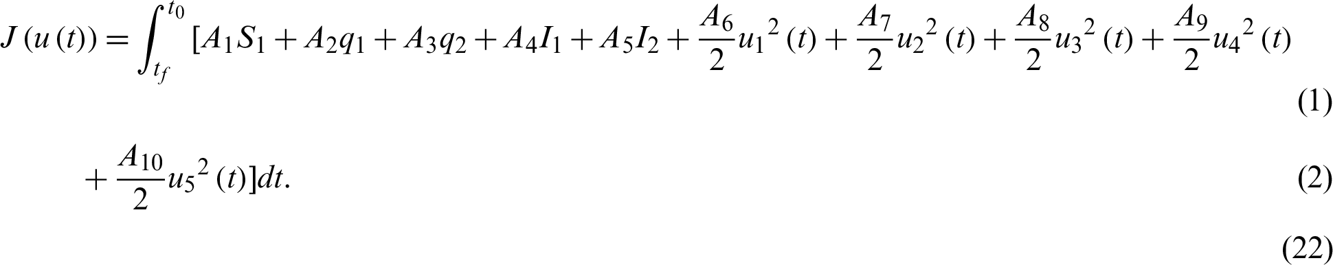
where,

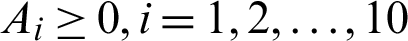denote the weights parameters that balanced the size of the terms.

We seek for optimal control u* such that

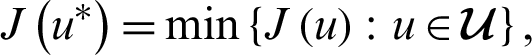
where

is the set of admissible controls defined by

4.2 Existence of Optimal Control

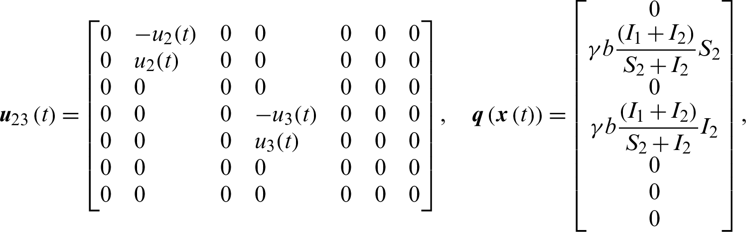
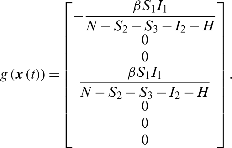
The system of nonlinear ODE Eqs. (15)–(21) can be written as,

where,

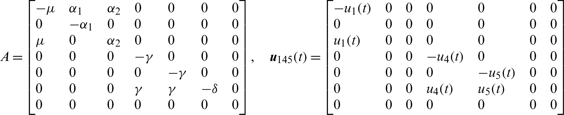
Theorem 3: The optimal control system Eq. (23) is Lipschitz continuous.

Proof

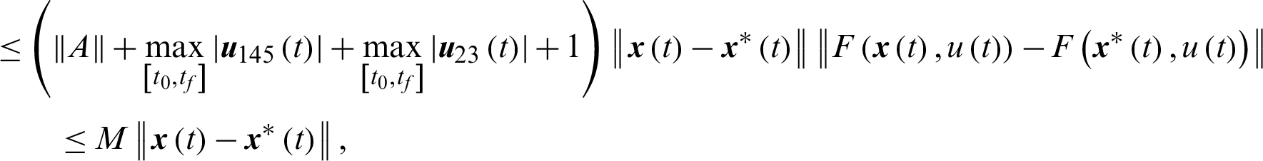
where,

4.3 Characterization of Optimal Control

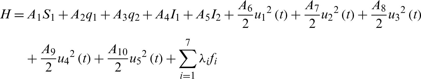
To formulate the optimal control strategy, we define the Hamiltonian as:

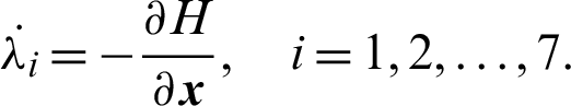
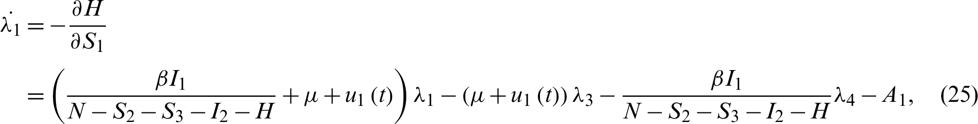
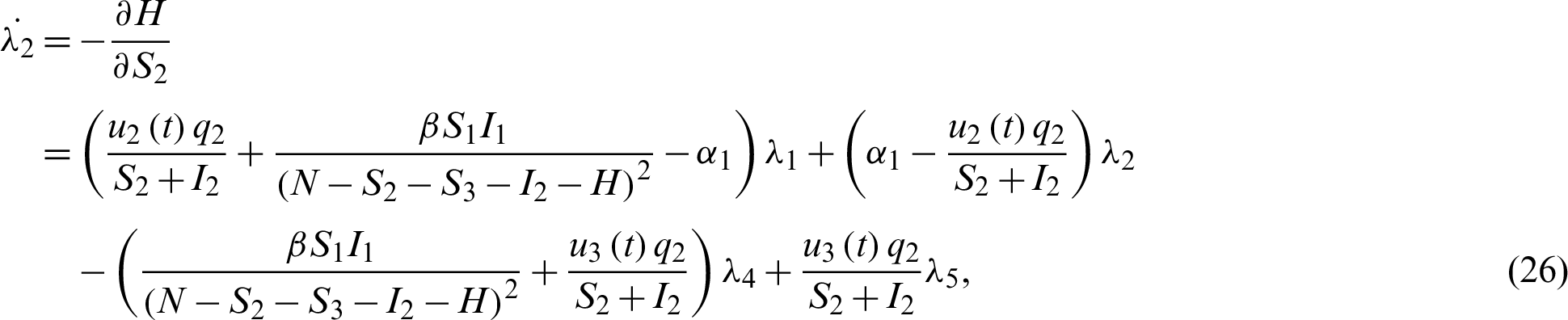
Theorem 4: Let with associated optimal control variables u1, u2, u3, u4, u5, then there exists a co-state variable satisfying:

Proof:

Applying the co-state (adjoint) condition of Eq. (5) yield

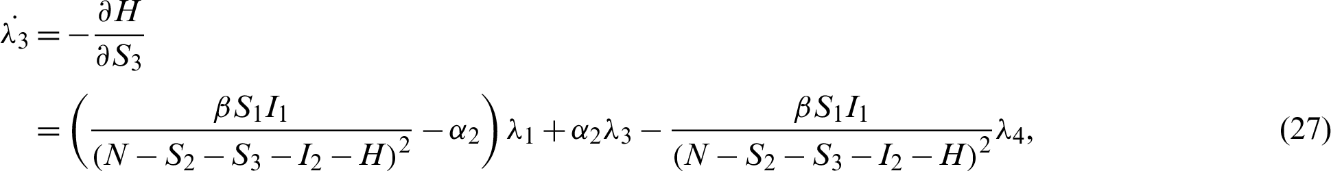
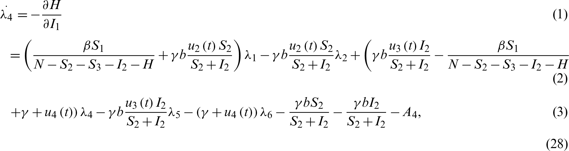
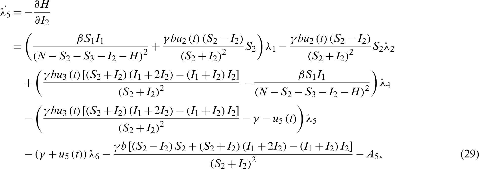
subject to the following transversality conditions;

Applying the optimality conditions, we get

Solving the optimality system requires initial and transversality conditions together with characterization obtained in Eqs. (38)–(42), in addition, from the Largrangian equation

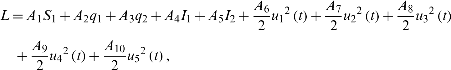
we can see that the second derivative with respect to is positive. This shows that the optimal control problem is minimum at controls respectively.

Now by substituting Eqs. (38)–(42) into the system Eqs. (15)–(21) we have;

5  Stability Analysis

In this chapter, two equilibrium points; Disease Free and Endemic Equilibria are found. Basic reproduction ratio is obtained. Global stability analyses of the equilibrium solutions are carried out.

5.1 Equilibria

Since there does not appear the state variable R in Eq. (15) through Eq. (21), it suffices to analyze the system Eq. (15) through Eq. (20).

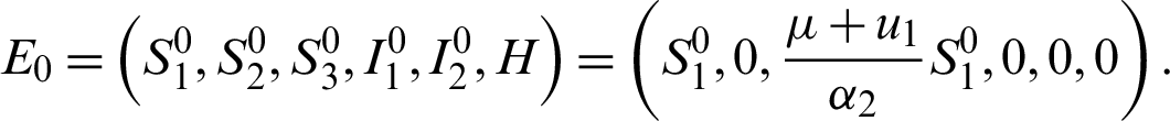
Disease free equilibrium E0 is obtained by substituting I1 = I2 = H = 0 into Eqs. (15)–(20), thus we have

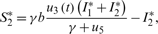
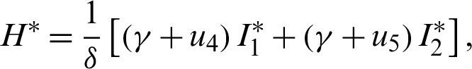
The endemic equilibrium 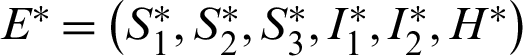is obtained when , , thus

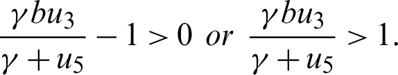
Since the endemic equilibrium is positive, then 0 i.e.,

or

Also

5.2 Local Stability of the Equilibria

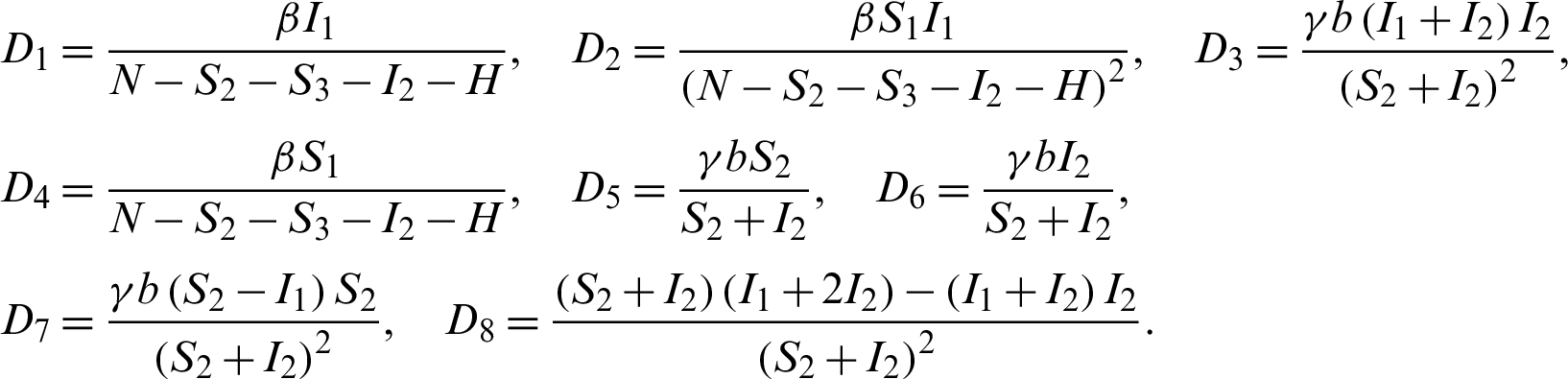
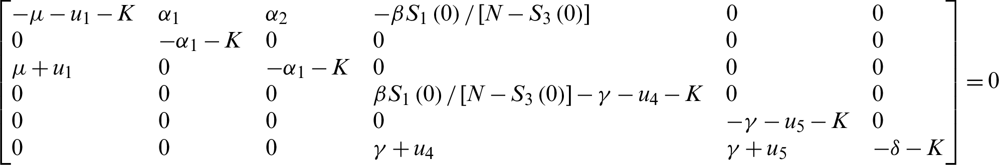
We construct the Jacobian matrix from Eqs. (15)–(20) as:

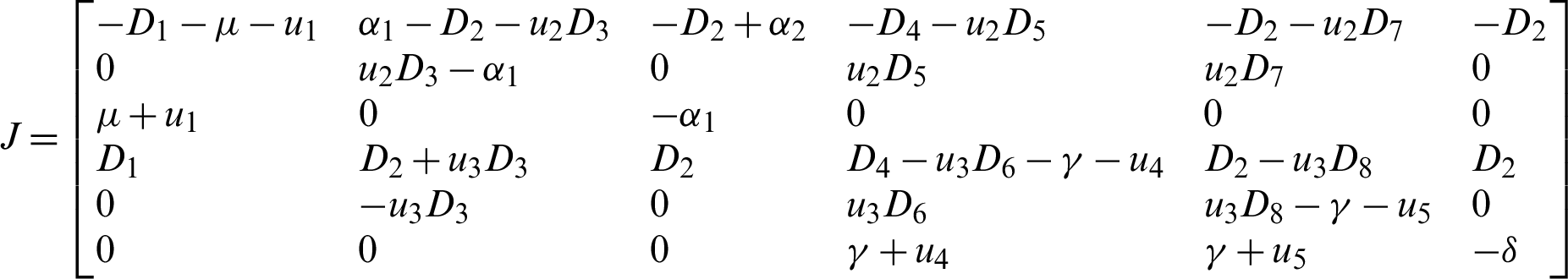
where,

Theorem 5: The disease free equilibrium E0 is locally asymptotically stable.

Proof:

The eigenvalue is obtained from;

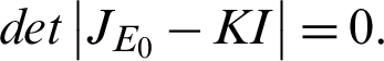
This implies;

5.3 Basic Reproduction Number

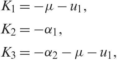
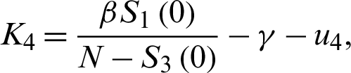
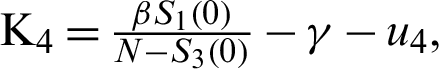
For the DFE to be locally asymptotically stable, the eigenvalue K4 must be negative. That is:

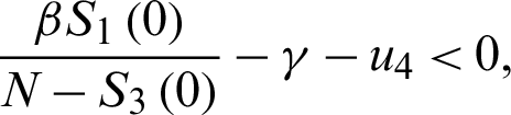
or

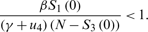
Now, define the basic reproduction ratio (R0) to be:

5.4 Global Stability Analysis

Here the global stability analyses of the two equilibrium points are carried out.

Theorem 6: The disease free equilibrium is globally asymptotically stable.

Proof:

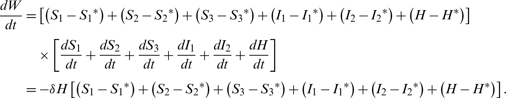
Let the Lyapunov candidate function be,

Clearly the above function .

Also , if

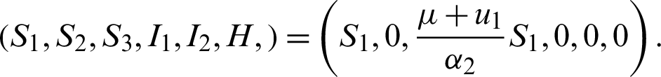
Clearly,

Theorem 7: The endemic equilibrium is globally asymptotically stable.

Proof:

Let the Lyapunov candidate function be,

Clearly, 0.

Also , if

Clearly,

6  Numerical Simulations

In this chapter numerical simulations are carried out to support the analytic results and to show the significance of the controller. Most of the data used in the simulation for the parameters and the variables is from china as in [7]. The values can be found in Tabs. 1 and 2 below.

Table 1: Model variables, descriptions and values

Table 2: Model parameters, descriptions and values

It can be seen from Fig. 2, that when no any control measure is observed and people were allowed to behave as usual the number of infected individuals will escalate. On the other hand if the control measures were observed optimally, that is; susceptible communities are isolated, susceptible individuals that have contact with infected individuals are quarantined, asymptomatic individuals are quarantined, and infected individuals are traced and hospitalized, then the number of infected individuals will drastically be reduced as shown in Fig. 3.

Figure 2: Dynamics of the infected population when there is no control

Figure 3: Dynamics of the infected population when all control measures are optimally observed

Although these control measures aren’t easy to be observed but their significance can easily be seen from the above graphs. It is clearly shown that when individuals and governments at various levels put hands together the spread of the disease will be curbed. From the above two graphs it can be seen that the number of people that will be removed from the population (either by death or by natural recovery) will be reduced from about when there is no control to less than 9000 people when control is observed optimally.

Acknowledgement: We thank the reviewers for their valuable contributions.

Funding Statement: The author(s) received no specific funding for this study.

Conflicts of Interest: The authors declare that they have no conflicts of interest to report regarding the present study.

This work is licensed under a Creative Commons Attribution 4.0 International License, which permits unrestricted use, distribution, and reproduction in any medium, provided the original work is properly cited.