DOI:10.32604/cmc.2021.012315
| Computers, Materials & Continua DOI:10.32604/cmc.2021.012315 | |
| Article |
An Optimal Deep Learning Based Computer-Aided Diagnosis System for Diabetic Retinopathy
1Department of Project Management, Ho Chi Minh City Open University, Ho Chi Minh City, 7000000, Vietnam
2Department of Learning Material, Ho Chi Minh City Open University, Ho Chi Minh City, 7000000, Vietnam
3Department of Convergence Science, Kongju National University, Gongju, 32588, South Korea
4Department of Computer Science and Engineering, Sejong University, Seoul, 05006, South Korea
*Corresponding Author: Eunmok Yang. Email: emyang@kongju.ac.kr
Received: 25 June 2020; Accepted: 29 July 2020
Abstract: Diabetic Retinopathy (DR) is a significant blinding disease that poses serious threat to human vision rapidly. Classification and severity grading of DR are difficult processes to accomplish. Traditionally, it depends on ophthalmoscopically-visible symptoms of growing severity, which is then ranked in a stepwise scale from no retinopathy to various levels of DR severity. This paper presents an ensemble of Orthogonal Learning Particle Swarm Optimization (OPSO) algorithm-based Convolutional Neural Network (CNN) Model EOPSO-CNN in order to perform DR detection and grading. The proposed EOPSO-CNN model involves three main processes such as preprocessing, feature extraction, and classification. The proposed model initially involves preprocessing stage which removes the presence of noise in the input image. Then, the watershed algorithm is applied to segment the preprocessed images. Followed by, feature extraction takes place by leveraging EOPSO-CNN model. Finally, the extracted feature vectors are provided to a Decision Tree (DT) classifier to classify the DR images. The study experiments were carried out using Messidor DR Dataset and the results showed an extraordinary performance by the proposed method over compared methods in a considerable way. The simulation outcome offered the maximum classification with accuracy, sensitivity, and specificity values being 98.47%, 96.43%, and 99.02% respectively.
Keywords: Diabetic retinopathy; convolutional neural network; classification; image processing; computer-aided diagnosis
In recent years, Diabetic Retinopathy (DR) is one of the major problems faced by many individuals that primarily affect the human vision. There are few ophthalmology-related diseases like diabetes, hypertension, and arteriosclerosis, which are considered to be the major reason behind blindness. Many professionals examined the modification of vascularmorphology by portioning the retinal vessels. Thus, the segmentation of DR images plays a crucial part in the diagnosis of relevant diseases. Some of the clinical images, in the form of 2-D color fundus images as well as 3-DOptic Coherence Tomography (OCT) images, are often applied for ophthalmic disease. The color fundus image can be retrieved conveniently using a fundus camera with the help of contrast to OCT image. This is generally used when analyzing the ophthalmologic diseases. In general, the experts partition the retinal vessels from fundus images manually. But the manual segmentation of images is a time-consuming process and non-scalable in practice. To overcome the limitations, efficient automated vessel segmentation is critically needed.
Computer-Aided Diagnosis (CAD) models have been developed to diagnose the disease in an automated manner. Such models are used to segment the images in an automated manner independent of professionals as well as it can offer flexible and powerful segmentation. But, this automation has been influenced by various aspects such as lesion region, complex vessel structure, and lower contrast of target and background, which altogether makes the segmentation process a more promising issue. Besides, the predefined segmentation models are classified as either supervised or unsupervised module which is based on manually-named ground truths. It is already known that the unsupervised models are developed based on the inherent nature of blood vessels with no manually-labeled maps [1].
Neto et al. [2] deployed an unsupervised model that segments the vascular structure based on arithmetic morphologies, spatial dependencies, curvatures, and so on. Khan et al. [3] projected an effectual contrast sensitive segmentation model by applying backdrop normalization, 2-order Gaussian filter, and region development. It mainly focused on minimum-contrast area of contrast sensitive. Zhao et al. [4] implied an indefinite perimeter active contour method which was used in case of Lebesgue estimation to predict the tiny vessels. This model helped in the integration of area information to ensure the prediction of vessels as well as vessel edges. Salazar et al. [5] processed an image pre-processing technique by adaptive histogram equalization as well as longer distance transform and portioned the vessels using graph cut.
Yin et al. [6] presented an approach to segment the images by applying Hessian matrix as well as threshold entropy. This approach made use of post-processing model to remove noise and central light reflex. Such models compute the output while predicting the retinal vessel based on vascular structure and few predefined information with no application of ground truths. Simultaneously, supervised frameworks obtain retinal blood vessels by understanding the patterns from annotation outcome. Marin et al. [7] declared the segmentation process as a pixel classification issue. Initially, the grey level is extracted while the moment invariant parameters for all the pixels are induced for Neural Networks (NN) to divide the pixels. Zhu et al. [8] produced discriminative feature vectors like local features, Hessian, and diverging vector field of all pixels which rely on prior information and Extreme Learning Machine (ELM) classifier model. In general, several techniques are developed based on prior knowledge to obtain discriminative features. Convolution Neural Network (CNN) is capable of providing automated learning of hierarchical features with the help of few convolutions as well as pooling functions when there is no prior knowledge and additional preprocessing [9,10].
CNN has been applied effectively in computer vision, clinical image processing, object tracking, and other areas. Wang et al. [11] portioned the retinal vessels by relying on the pixel classifying mode. A hierarchical segmentation model applied CNN as a training feature extracting device as well as used the ensemble Random Forests (RFs) as a training classifier model. To compute the pixel class, it obtained the features from a square sub-window that is centralized on pixel. This is essential to classify the CNN while the pixel class is detected using ensemble RFs. Such types of patch-based techniques are said to be time consuming processes since maximum amount of repeated measures are followed in it. Moreover, the available image-to-image CNN approach performs better in the prediction of wider objects. But the retinal structure is often thin yet elaborated, and is very hard to segment the vessels with exact accuracy. Also, the imbalance issue gets improved with the complexity of dividing the vessels since these 10% of these vessel images are used in the whole image.
Xie et al. [12] suggested a retinal vessel segmentation process as a boundary prediction operation. In the beginning, Holistically-nested Edge Detection (HED) was used in the study to obtain possible mapping while a Fully Connected (FC) Conditional Random Field (CRF) was applied to clarify the segmentation function. The image-to-image technique is highly effective and accurate segmentation value was obtained. By improving the network layer, the receptive field gets slowly enhanced to learn the maximum global discriminative features so as to isolate the vessels and non-vessels. Therefore, top layers are composed of maximum amount of global data whereas the bottom layers are involved with much information. This model tended to leave few vascular edges as well as thin vessels by acquiring the portion of top layers. This helps to assure the precision of entire structure that tend to be highly vascular.
A new DR classification model, to identify the different classes of DR images, has been developed in the literature [13]. The proposed method determines the severity of diseases using CNN by incorporating Pooling, Softmax, and Rectified Linear Activation Unit (ReLU) layers to obtain high level of accuracy. The simulation of this model was performed on Messidor database. Wan et al. [14] developed an automated classification model to categorize a set of fundus images using the CNN model. Coupled with transfer learning and hyper-parameter tuning, various models such as AlexNet, VggNet, GoogleNet, and ResNet models were analyzed on the classification process of DR images [15,16].
Several CNN models are available in the literature to understand the discriminative data by maximizing the network depth, where the information with shallow layers could not be rejected to detect the thin prolonged vascular structure [17]. To be specific, image pixels can be classified into two levels: simple to forecast, and complex to predict. Since a simple pixel fills more space in fundus images, it is dominated by the dimension of the parameter at the time of training the CNN. Yet, there is a constraint that it has not been predicted exactly while the loss is stabilized and the CNN technique ignores to update. Darwish et al. [18] conducted a study where the hyperparameter optimization of CNN was performed using Orthogonal Learning Particle Swarm Optimization (OLPSO) algorithm. The OLPSO algorithm performed effective hyperparameter optimization by identifying the optimum values instead of using classical models like manual trial and error method. This research work prevented the CNNs from falling into local minimum and trained the CNNs efficiently. This method also avoided the local optima problem of OLPSO algorithm and performed effective training process. Due to these positive characteristics, the OLPSO algorithm has been utilized in the current study to perform effective feature selection so as to diagnose DR.
This paper presents an ensemble of Orthogonal Learning Particle Swarm Optimization algorithm (OPSO)-based Convolutional Neural Network (CNN) model EOPSO-CNN so as to perform DR detection and grading. The proposed EOPSO-CNN model involves three main processes such as preprocessing, feature extraction, and classification. The proposed model initially involves preprocessing stage which removes the presence of noise in the input image. Then, the watershed algorithm is applied to segment the preprocessed images. Followed by, feature extraction takes place by leveraging EOPSO-CNN model. Finally, the extracted feature vectors are provided to a Decision Tree (DT) classifier to classify the DR images. The experiments were carried out using Messidor DR Dataset and the results showed an extraordinary performance by the proposed method over compared methods in a considerable way.
The remaining sections of the paper are arranged as follows. Section 2 explains the proposed EOPSO-CNN model and Section 3 provides the performance validation. At last, Section 4 draws the conclusion.
The working principle of the proposed model is shown in the Fig. 1. The proposed EOPSO-CNN model involves three main processes such as preprocessing, feature extraction, and classification. Initially, the preprocessing is applied in order to remove the noise in the input image. Followed by, watershed-based segmentation process is carried out. Then, feature extraction is performed using EOPSO-CNN model. Finally, the extracted feature vectors are provided to a DT classifier to classify the DR images.
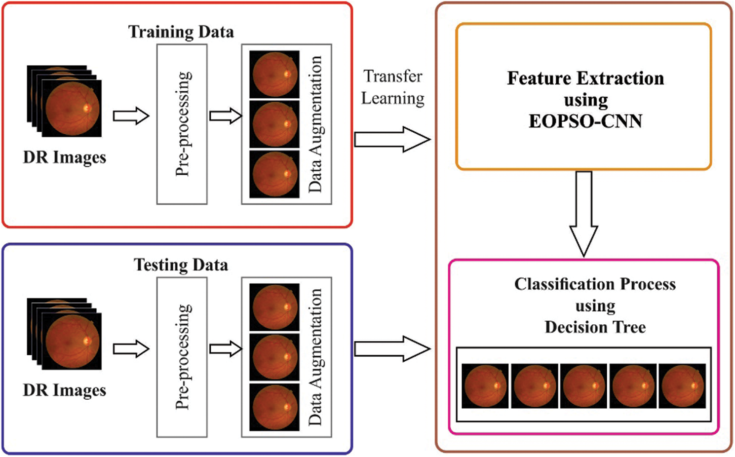
Figure 1: The overall process of the proposed work
2.1 Preprocessing and Augmentation
It is the most important stage that discards several kinds of noises. At first, the DR images are regularized. To obtain high accuracy, CNN needs large dataset since the action of CNN declines with small datasets due to over-fitting. It implies that the network executes thoroughly on trained data although it under-executes on testing data. Using the presented structure, data augmentation methods are used to increase the dataset and decrease over-fitting problems. If data augmentation technique gets heavily implemented, the number of instances gets raised with executing geometric conversions to the image data sets utilizing easy image processing methods. Based on the above, the image dataset is raised with color processing, transformation, flipping, and noise perturbation. While DR images are rotationally invariant, the pathologist simply analyzes the DR images from various angles without much differences in the analysis. The total number of images in MESSIDOR dataset is 1200 while the possible data augmentation process is performed using image DataGenerator function of Keras library to resize and rescale the sample images. The data augmentation values of different approaches are given here: Rotation: 30, Width shift: 0.2, Height shift: 0.2, Shear: 0.1, Zoom: 0.3, Horizontal flip: True and Fill mode: Nearest.
Watershed segmentation techniques depend upon the representation of images in the form of a topographic relief. In this, the value of every image component defines the height at this point. It processes both 2D and 3D images. Therefore, the term ‘element’ is utilized for combining the terms, pixel and voxel. To attain effective performance, watershed segmentation is frequently employed to the outcome of distance transform of the image, instead of the actual image. Hence, the relief comprises of low-lying valleys (minimums), high-altitude ridges (watershed lines) and slopes (catchment basins). The idea of a plateau (an area with the same height of elements) is employed herewith. The major function of segmentation is to compute the position of every catchment basin and/or watershed lines. This is because, in this case, every catchment basin is treated as an individual segment of the image.
In the past decades, CNN has been developed significantly in major applications to solve problems that are related to image classification. CNN models are the most precise tools which have been applied to forecast features obtained from input images [19–27].
CNN consists of a collection of layers applied in the discovery of image features. The most essential layers are convolutional layer, activation layer, batch normalization layer, and pooling layer. First, the convolutional layers are assumed to be a required unit in CNN structures. The layers are comprised of a set of filters to discover the existence of particular features that can be applied in image characterization like edges and textures named feature maps. Next, the activation layers are employed to process non-linear transformations to find the outcome of prior convolutional layer with the application of activation function, i.e., Rectified Linear Unit (ReLU). ReLU has commonly employed the activation functions since it provides quick processing and exhibits no problem of exploding issues. ReLU can be expressed as:

where the gradient in terms of input can be defined by:

Batch normalization layers attempt to minimize the count of training epochs that are required in network training. It also enhances the function by rescaling each scalar feature  with a limited mini-batch
  based on Eq. (3).

where  refers a small positive value to terminate the division by 0,
  is a mini-batch mean which can be determined with the help of Eq. (4), and
  implies a mini-batch variance which is measured by Eq. (5).


While executing batch normalization, two novel attributes, γ, and β, are generally included to allow scaling and shifting-generalized inputs based on Eq. (6). Such attributes are learned with network features.

The pooling layers focus on reducing the perimeter of feature maps to decide an important and viable feature so as to minimize the number of parameters as well as processing of the network.
Here, PSO models are effectively applied in different optimization domains. The major disadvantage of PSO technique is its termination from local minima with few limitations in resolving high-definition issues. Hence, a novel method named ‘OPSO’ derived by Darwish et al. [18], was employed in this study to solve the embedded demerits of PSO. Furthermore, the learning principle of PSO depends upon every particle from a swarm that attain two powerful solutions. One instance of the issues is the presence of residual particles from a global optimum. Additionally, PSO model consists of some attributes which are applied in this regard. The oscillation of particles occur from PSO as well as projected neoteric principle by employing an integrated vector in accordance to the integration of personal best as well as global best vectors. Hence, the particle of swarm in PSO is comprised of a single active group and passive group. From an active group, the particles are upgraded on the basis of Orthogonal Diagonalization (OD) process, which has the position vectors of particles in the place of orthogonally-diagonalized location [28]. OPSO is an extended model of PSO which can overcome the demerits of global PSO and enhance the function of PSO. The OPSO methods function on the basis of leveraging OD operation. The orthogonal guidance vectors could be attained from an active group. Also, OD process achieves a Diagonal Matrix, DM, by transforming a product of three matrices. Here, the DM is applied to extend the vectors of velocity as well as the position for every particle of the swarm. Hence, the extension task could be provided with the help of ith vectors of velocity and position by a single diagonal element,  of DM.
The process of OD is capable of providing an optimal solution and boosts the converging outcome in search space. DM is attained by transforming the square matrix  , which contains
  size, as a diagonal matrix termed as DM with size of
  as given below:

where  denotes a matrix with eigenvector of
  and size of
  . The matrix
  is an invertible matrix which can be presented as follows:

The columns are orthogonal for one another in matrix  . Hence, the equation is expressed as.

where  refers the orthogonal matrix; hence, the equation is modified as:

However, the equation expresses the OD function.
The OPSO technique is applied with CNN in order to resolve the optimization of hyper-parameters in CNN [18], where OPSO model offers a novel method in swarm population. The swarm population is comprised of  particles. All the particles consist of dimensions. According to OD,
  particles are classified into two sets namely active and passive groups. The OPSO method is explained as follows. Assume
  refers to a function which must undergo optimization as well as iteration at the time of conducting a search process as defined by
  . The OPSO steps are defined in a step-by-step process as follows:
i. Initiate the position of the vector  and velocity
  for all the particles randomly
ii. Apply the position vector  to measure the objective function
  .
.
iii. Initiate a personal position vector of a particle  in PSO model using a function:

where  is the personal experience. Employ the function to compute personal position vectors.
iv. Arrange the m personal position vectors in an increasing manner, according to the fitness value of hx.
v. Develop matrix  that has size
  . This matrix consists of every row, which has
  personal position vectors in a similar ordered sequence similar to step 4.
vi. Employ PSO pseudo-code to transform matrix  to symmetric matrix
  that has the size of
  .
.
vii. Use OD on matrix  to attain a diagonal matrix
  along with size
viii. Upgrade the vectors of position as well as velocity of  particles in an active group using the given functions:


where  is the
  raw of matrix
  represents a coefficient of acceleration and is selected by applying trial and error in the interval of [2,2.5].
ix. By applying the following Eq. (14), compute the  from
from  particles as given:

Then calculate 
x. Compute the optimal position. Choose  with respect to lower
Then estimate  to evaluate the best position,
  , where

xi. End the iterations, 
The  is determined in step 10 to offer the best solution.
2.4 Decision Tree (DT) Classifier
For classification purposes, DT classifier is applied over other classifiers due to the following merits. It is simple to implement and generate understandable rules. It requires less computation to carry out the classification process. It does not need data normalization and data scaling whereas the missing values in the data do not have any impact in building a DT to a certain extent. The DTs are developed models to divide the group of items into a number of classes [29]. A DT is capable of classifying data items in a definite number of predetermined classes. The tree nodes are modeled with attributes and arcs are labeled with viable measures of the attribute whereas the leaves are named with diverse classes. ID3 system is previously a Data Mining (DM) model. An item undergoes classification using a path and tree, developed by the arcs in terms of values, to corresponding attributes. Predecessors of ID3 applied in the development of DTs are C4.5. The provided set  of items, i.e., C4.5 initially develops a DT with the help of divide-and-conquer technique as given below:
• When every item in C comes under a similar class or C is less, the tree is named as a leaf with common frequent class in C.
• Else, select a sample based on one-parameter with maximum number of results. In the test of root with a single branch for all outcomes of a test, partition the C into a set of subsets  based on the result of every item. It uses a similar pattern recursively for all the subsets.
Various tests can be applied in the last step. C4.5 utilizes two heuristic criteria for ranking feasible tests: information gain reduces the complete entropy of subsets , and basic gain ratio helps in the division of data gained by information given by sample results.
The parameters which compute the test results might be arithmetic or nominal. For a mathematical attribute  where the threshold
  that sorts
  on
on  , a split is selected from successive measures as it improves the performance. An attribute
  , with discrete rates, is composed of a fundamental resultant value that enables the values to be collected as the maximum count of subsets with single simulation outcome for all the subsets.
Initially, the first tree undergoes pruning to eliminate the problem of over-fitting. The pruning model depends upon a negative estimation of error value correlated with a group of N cases whereas Z does not come under the frequent category. By replacing  , C4.5 computes an upper limit of binomial probability at the time of observing the Z actions in N trials, on the basis of user-specified confidence with basic values. Pruning is carried out from leaf to root. The calculated error from a leaf along with N items as well as Z errors is N times of pessimistic error value. In a sub-tree, C4.5 includes measured errors of branches and determines the error, when a sub-tree is interchanged by a leaf. When an alternate tree is maximum than the first one, a sub-tree has to be pruned. Likewise, C4.5 validates the estimated error, while a sub-tree is substituted by a single branch that provides the merits of the tree accordingly. The pruning process can be completed in a single pass by a tree.
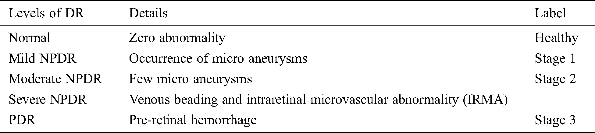
For assessing the outcome of the projected method, a standard MESSIDOR dataset [30] was used consisting of 1,200 color fundus images along with proper annotation. The proposed model is implemented by the use of Python 3.6.5 tool along with few packages. These images exist in the dataset classified as a group of four levels as depicted in the Tab. 1. Some images are constrained with few micro aneurysms that come under stage 1. The images with micro aneurysms as well as hemorrhages belong to stage 2 and images present with the maximum number of micro aneurysms and hemorrhages come under stage 3. For experimentation, 10-fold cross validation process is employed.
A collection of four evaluation features such as sensitivity, specificity, accuracy as well as precision factor was applied to consume the function of the presented method. The functions applied to compute the value has been offered in Eqs. (1)–(3):

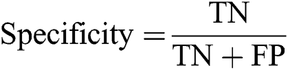

Fig. 2 displays the visualization produced as a result of the proposed method. As illustrated in the Fig. 2a. it reveals the sample input color fundus images that are segmented efficiently and classified effectively. Fig. 2b demonstrates the divided outcome of the used sample images and the classified image is shown in the Fig. 2c.
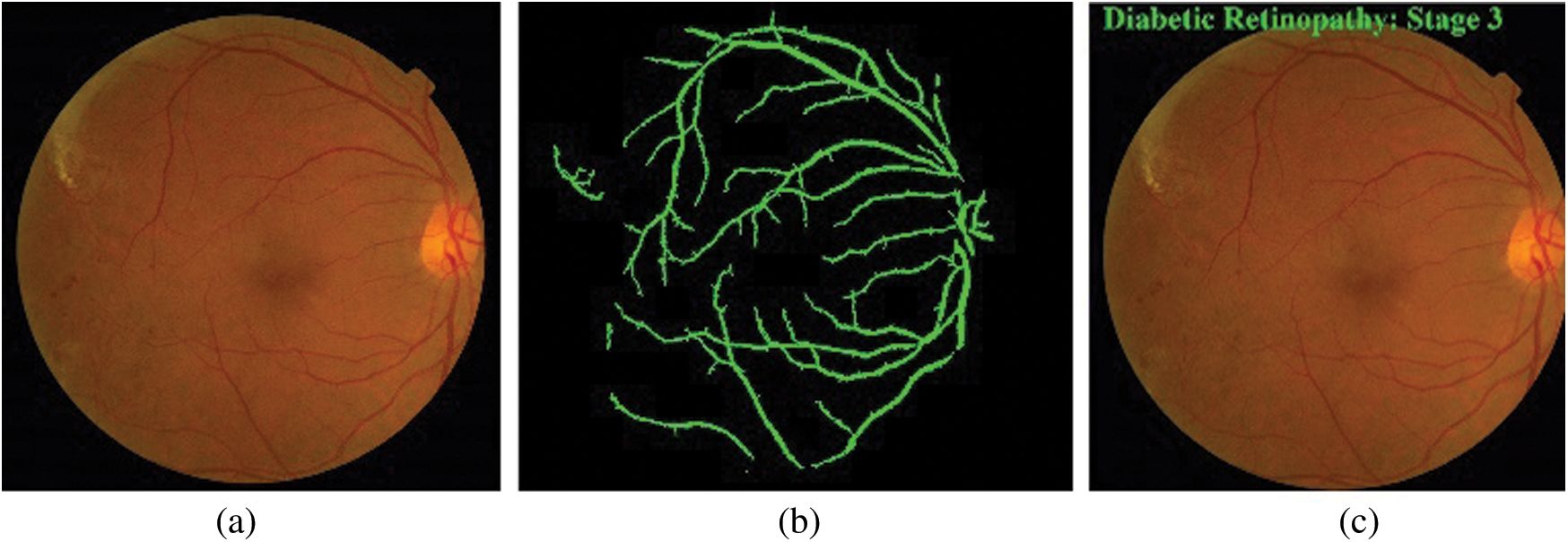
Figure 2: a) Original image, b) Segmented image, c) Classified image
Tab. 2 shows a sample set of visualization of the results achieved by the proposed model. It is established that the proposed model effectively segmented and clarified different stages of DR images. Tab. 3 shows the confusion matrix that was generated at the time of execution by EOPSO-CNN model. The values present in the table are transformed into values such as True Positive (TP), True Negative (TN), False Positive (FP) and False Negative (FN), as shown in the Tab. 4 as well as in Figs. 3 and 4. These values were considered to determine the classification performance of the proposed model.
Table 2: The sample visualization of classified results
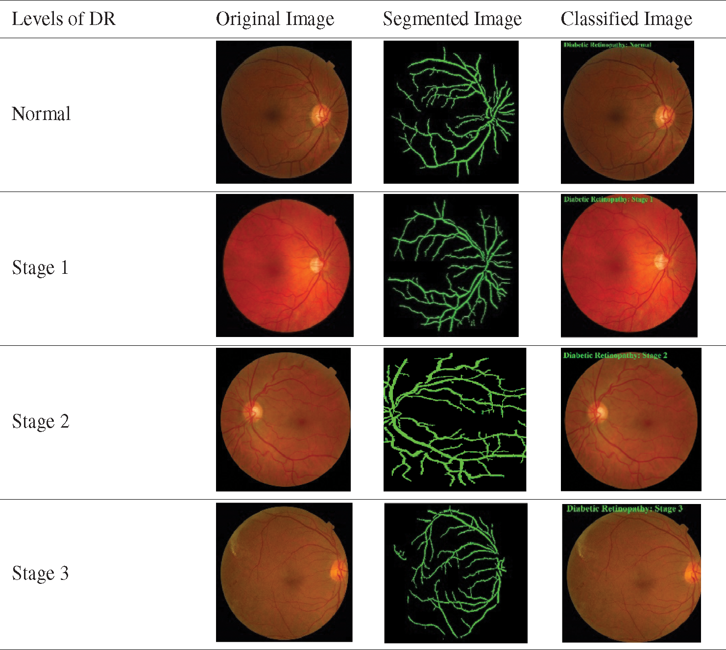
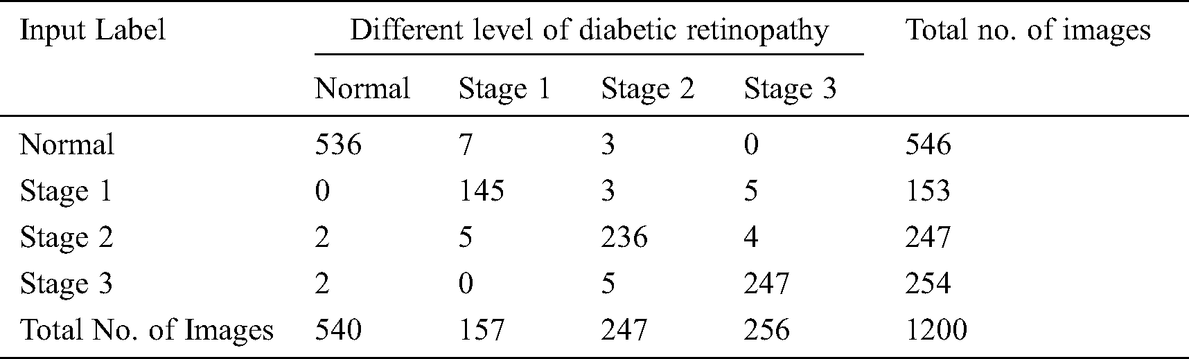
Table 4: Manipulations from confusion matrix
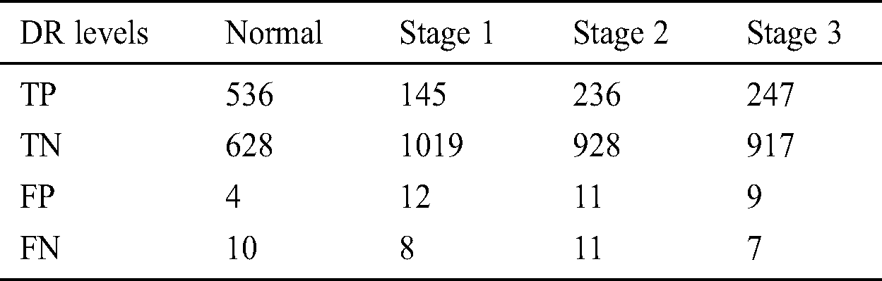
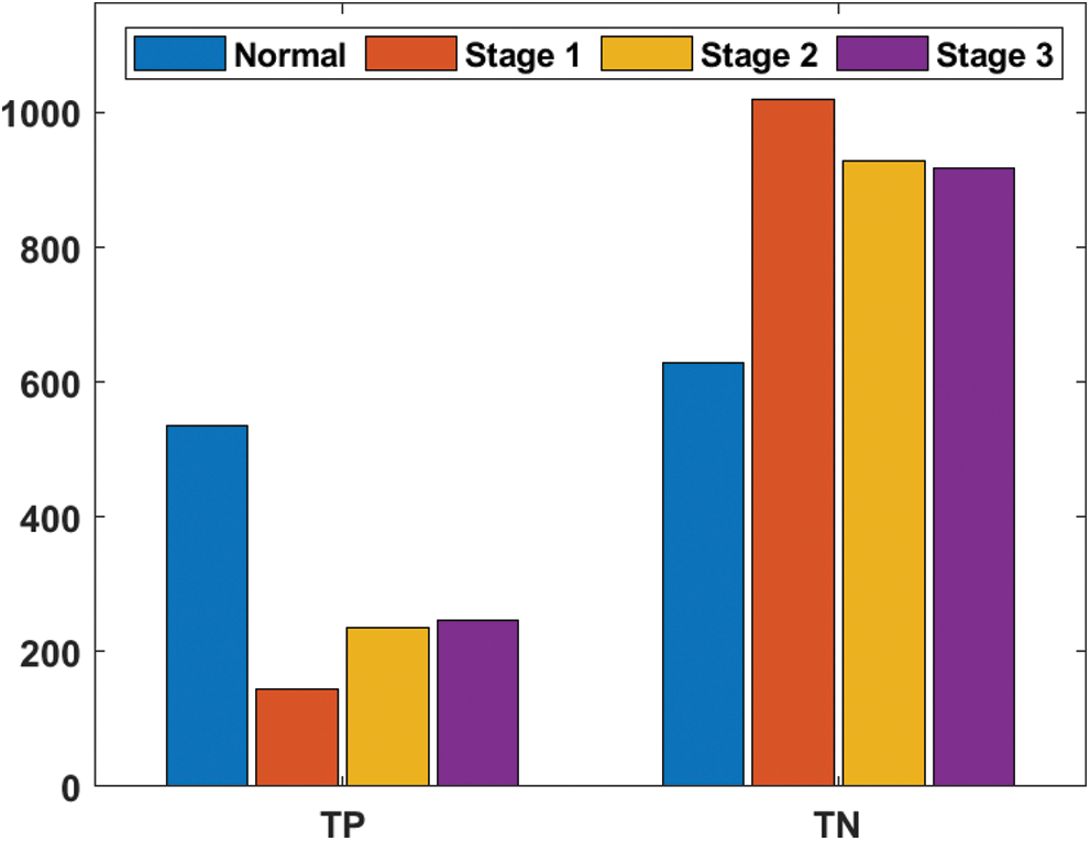
Figure 3: TP and TN analysis of EOPSO-CNN model
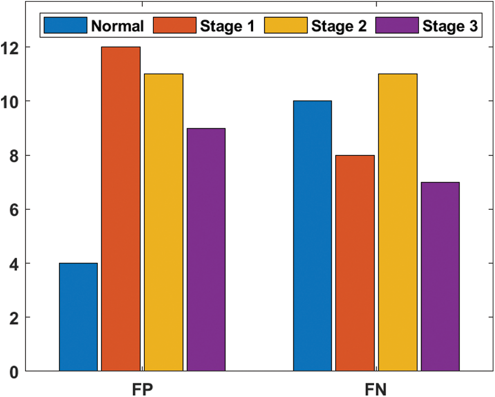
Figure 4: FP and FN analyses of the EOPSO-CNN model
Tab. 5 and Figs. 5–6 demonstrate the results offered by EOPSO-CNN model when classifying the DR images. During the classification of normal images, the normal images were classified with the maximum sensitivity of 98.17%, specificity of 99.37%, accuracy of 98.81% and precision of 99.26%. At the same time, during the classification of stage 1 images, the test images were classified with the maximum sensitivity of 94.77%, specificity of 98.84%, accuracy of 98.31% and precision of 92.36%. In the same way, during the classification of stage 2 images, the applied images were classified with the maximum sensitivity of 95.55%, specificity of 98.83%, accuracy of 98.15% and precision of 95.55%. Finally, during the classification of stage 3 images, the normal images were classified with the maximum sensitivity of 97.24%, specificity of 99.03%, accuracy of 98.64% and precision of 96.48%.
Table 5: Performance measures of test images with different DR levels
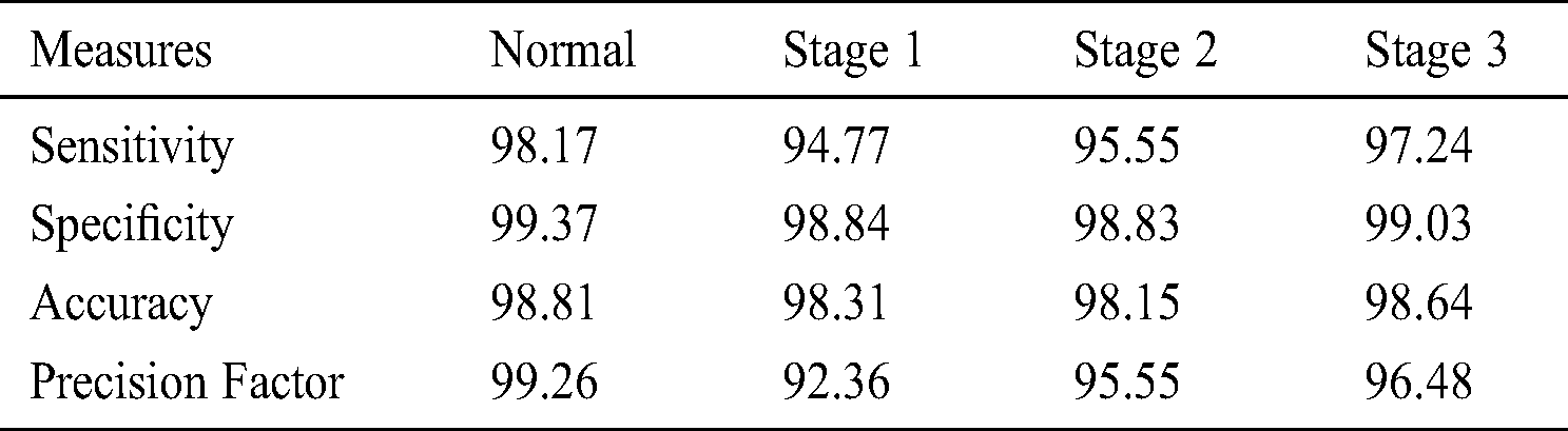
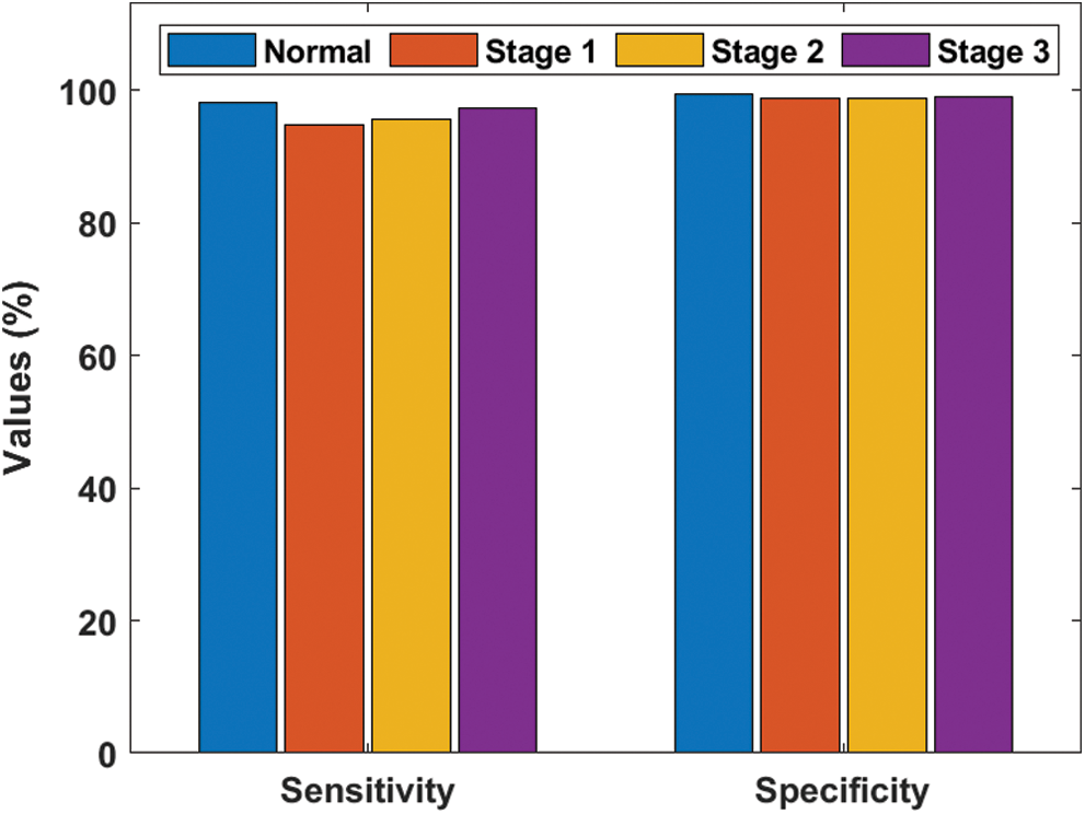
Figure 5: Sensitivity and specificity analyses of EOPSO-CNN model
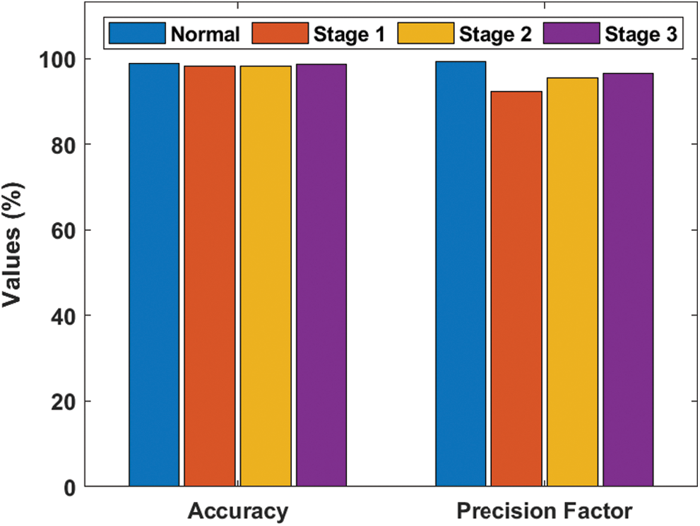
Figure 6: Accuracy and precision analyses of EOPSO-CNN model
Tab. 6 and Figs. 7–9 offers a detailed comparative analyses of different models [13,14] in terms of accuracy, sensitivity and specificity. As shown in the Fig. 7 by calculating the classification result with respect to accuracy, it can be inferred that the AlexNet method attained poor classification by obtaining lower accuracy of 89.75%. Simultaneously, the ResNet approach yielded a slightly better classification by achieving gradual accuracy of 90.40%.
Table 6: Performance measures of test images with different DR levels
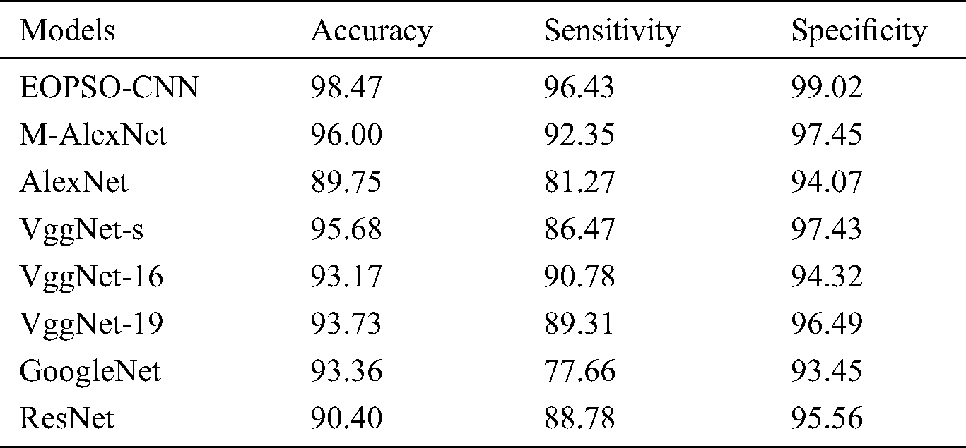
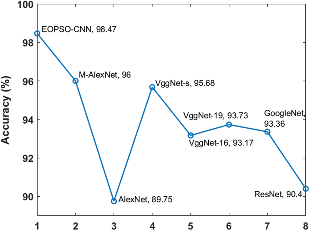
Figure 7: Comparative analysis of different models in terms of accuracy
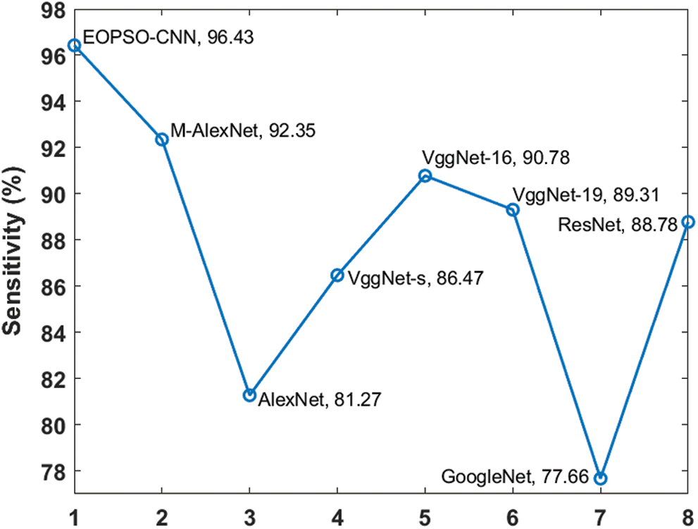
Figure 8: Comparative analysis of different models in terms of sensitivity
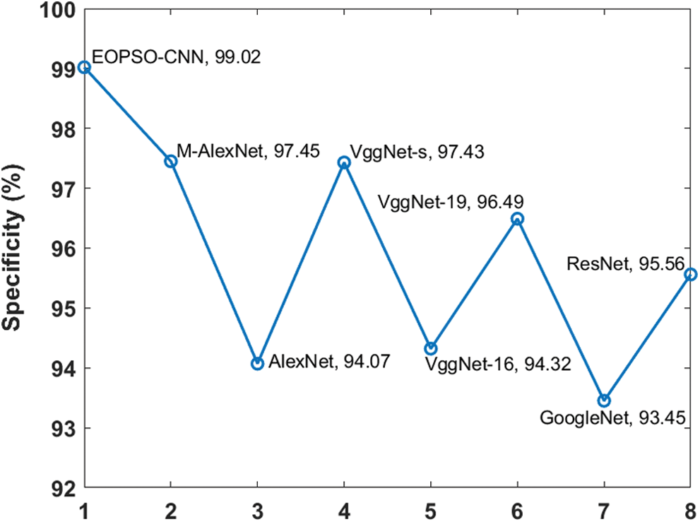
Figure 9: Comparative analysis of different models in terms of specificity
Followed by, VggNet-16, VggNet-19 and GoogleNet methods exhibited reasonable as well as adjacent outcomes by attaining accuracies of 93.17%, 93.73% and 93.36% respectively. Afterward, the VggNet-s technology depicted good results than the previous techniques by achieving an accuracy of 95.68%. Next, the M-AlexNet methodology illustrated comparative results by achieving the maximum accuracy of 96.00%. But, the proposed EOPSO-CNN method exhibited an outstanding classification process by attained the highest accuracy of 98.47%.
Fig. 8 shows a comparison of the sensitivity results of different models. When measuring the classification outcome in terms of sensitivity, it is reported that the GoogleNet model achieved worst sensitivity of 77.66%. Alternatively, the AlexNet technique offered a slightly better classification by accomplishing a lower sensitivity of 81.27%. Simultaneously, VggNet-s, ResNet and VggNet-19 techniques resulted in a considerable and nearby result by achieving the sensitivities of 86.47%, 88.78% and 89.31% respectively. Then, VggNet-16 exhibited a better outcome when compared with other models by producing the sensitivity of 90.78%. Subsequently, the M-AlexNet approach showcased appreciable results by obtaining good sensitivity of 92.35%. Again, the proposed EOPSO-CNN technique resulted in optimized classification task by attaining maximum sensitivity of 96.43%.
Fig. 9 displays a comparative examination of distinct models in terms of specificity. By estimating the classification outcome corresponding to specificity, it is understood that the GoogleNet technology achieved the least classification by getting minimum specificity of 93.45%. At the same time, the AlexNet scheme offered a gradual classification with specificity value being 94.07%. Next, VggNet-16, ResNet and VggNet-19 frameworks achieved manageable result by attained the specificity values such as 94.32%, 95.56% and 96.49% respectively. Followed by, the VggNet-s method demonstrated the best outcome in comparison with other models by attaining the specificity of 97.43%. Afterward, the M-AlexNet scheme accomplished a relative result by producing a reputed specificity of 97.45%.
However, the proposed EOPSO-CNN technique implied a standard classification operation by accomplishing the optimized specificity of 99.02%. The simulation outcome offered maximum classification with accuracy, sensitivity, and specificity values being 97.13%, 93.86%, and 99.02% respectively. Hence, the proposed EOPSO-CNN technique could be applied as an automatic diagnostic tool to classify the DR images.
An Optimal Deep Learning based Computer-aided Diagnosis System for Diabetic Retinopathy in this study. The project method consists of preprocessing stage which removes the noise in input image. Subsequently, watershed-based segmentation and feature extraction occur using the EOPSO-CNN model. Finally, the extracted feature vectors are provided to a DT classifier to classify DR images. The experiments of the study were carried out using Messidor DR Dataset and the results stated the presented model exhibited extraordinary performance over other compared methods in a considerable way. The simulation outcome offered the maximum classification with accuracy, sensitivity, and specificity values being 98.47%, 96.43%, and 99.02% respectively. In future, the outcome of the projected approach can be further improved by possibly using recently updated segmentation models.
Funding Statement: This work was supported by Sejong University new faculty research funds.
Conflicts of Interest: The authors declare that they have no conflicts of interest to report regarding the present study.
1 P. He, Z. L. Deng, C. Z. Gao, X. N. Wang and J. Li. (2017). “Model approach to grammatical evolution: Deep-structured analyzing of model and representation,” Soft Computing, vol. 21, no. 18, pp. 5413–5423. [Google Scholar]
2 L. C. Neto, G. L. B. Ramalho, J. F. S. Rocha Neto, R. M. S. Veras, F. N. S. Medeiros et al. (2017). , “An unsupervised coarse-to fine algorithm for blood vessel segmentation in fundus images,” Expert Systems with Applications An International Journal, vol. 78, no. C, pp. 182–192. [Google Scholar]
3 M. A. U. Khan, T. A. Soomro, T. M. Khan, D. G. Bailey and J. Gao. (2016). , “Automatic retinal vessel extraction algorithm based on contrast-sensitive schemes,” in 2016 Int. Conf. on Image and Vision Computing, New Zealand, pp. 1–5. [Google Scholar]
4 Y. Zhao, L. Rada, K. Chen, S. P. Harding and Y. Zheng. (2015). “Automated vessel segmentation using infinite perimeter active contour model with hybrid region information with application to retinal images,” IEEE Transactions on Medical Imaging, vol. 34, no. 9, pp. 1797–1807. [Google Scholar]
5 A. S. Gonzalez, D. Kaba, Y. Li and X. Liu. (2014). “Segmentation of the blood vessels and optic disk in retinal images,” IEEE Journal of Biomedical and Health Informatics, vol. 18, no. 6, pp. 1874–1886. [Google Scholar]
6 X. Yin, B. W. H. Ng, J. He, Y. Zhang and D. Abbott. (2014). “Accurate image analysis of the retina using hessian matrix and binarisation of thresholded entropy with application of texture mapping,” PLoS One, vol. 9, no. 4, pp. 1–17. [Google Scholar]
7 D. Marín, A. Aquino, M. E. G. Arias and J. M. Bravo. (2011). “A new supervised method for blood vessel segmentation in retinal images by using gray-level and moment invariants-based features,” IEEE Transactions on Medical Imaging, vol. 30, no. 1, pp. 146–158. [Google Scholar]
8 C. Zhu, B. Zou, R. Zhao, J. Cui, X. Duan et al. (2017). , “Retinal vessel segmentation in colour fundus images using extreme learning machine,” Computerized Medical Imaging and Graphics, vol. 55, pp. 68–77. [Google Scholar]
9 I. V. Pustokhina, D. A. Pustokhin, D. Gupta, A. Khanna, K. Shankar et al. (2020). , “An effective training scheme for deep neural network in edge computing enabled internet of medical things (IoMT) systems,” IEEE Access, vol. 8, no. 1, pp. 107112–107123. [Google Scholar]
10 J. S. Raj, S. J. Shobana, I. V. Pustokhina, D. A. Pustokhin and D. Gupta. (2020). “Optimal feature selection based medical image classification using deep learning model in internet of medical things,” IEEE Access, vol. 8, no. 1, pp. 58006–58017. [Google Scholar]
11 S. Wang, Y. Yin, G. Cao, B. Wei, Y. Zheng et al. (2015). , “Hierarchical retinal blood vessel segmentation based on feature and ensemble learning,” Neurocomputing, vol. 149, pp. 708–717. [Google Scholar]
12 S. Xie and Z. Tu. (2017). “Holistically-nested edge detection,” International Journal of Computer Vision, vol. 125, no. 1–3, pp. 3–18. [Google Scholar]
13 T. Shanthi and R. S. Sabeenian. (2019). “Modified alexnet architecture for classification of diabetic retinopathy images,” Computers & Electrical Engineering, vol. 76, pp. 56–64. [Google Scholar]
14 S. Wan, Y. Liang and Y. Zhangab. (2018). “Deep convolutional neural networks for diabetic retinopathy detection by image classification,” Computers & Electrical Engineering, vol. 72, pp. 274–282. [Google Scholar]
15 K. Shankar, A. R. WahabSait, D. Gupta, S. K. Lakshmanaprabu and A. Khanna. (2020). “Automated detection and classification of fundus diabetic retinopathy images using synergic deep learning model,” Pattern Recognition Letters, vol. 133, pp. 210–216. [Google Scholar]
16 K. Shankar, E. Perumal and R. M. Vidhyavathi. (2020). “Deep neural network with moth search optimization algorithm based detection and classification of diabetic retinopathy images,” SN Applied Sciences, vol. 2, no. 4, pp. 84. [Google Scholar]
17 Q. Li, W. Cai, X. Wang, Y. Zhou, D. D.Feng et al. (2014). , “Medical image classification with convolutional neural network,” in 13th IEEE Int. Conf. on Control Automation Robotics & Vision, Singapore, pp. 844–848. [Google Scholar]
18 A. Darwish, D. Ezzat and A. E. Hassanien. (2020). “An optimized model based on convolutional neural networks and orthogonal learning particle swarm optimization algorithm for plant diseases diagnosis,” Swarm and Evolutionary Computation, vol. 52, pp. 1–12. [Google Scholar]
19 S. R. Zhou, W. L. Liang, J. G. Li and J. U. Kim. (2018). “Improved VGG model for road traffic sign recognition,” Computers, Materials & Continua, vol. 57, no. 1, pp. 11–24. [Google Scholar]
20 Z. Tang, L. G. Jiang, L. Yang, K. L. Li and K. Q. Li. (2015). “CRFs based parallel biomedical named entity recognition algorithm employing MapReduce framework,” Cluster Computing, vol. 18, no. 2, pp. 493–505.
21 C. F. Feng, S. Arshad, S. W. Zhou, D. Cao and Y. G. Liu. (2019). “Wi-Multi: A three-phase system for multiple human activity recognition with commercial WIFI devices,” IEEE Internet of Things Journal, vol. 6, no. 4, pp. 7293–7304.
22 X. F. Wang, L. Wang, S. J. Li and J. Wang. (2018). “An event-driven plan recognition algorithm based on intuitionistic fuzzy theory,” Journal of Supercomputing, vol. 74, no. 12, pp. 6923–6938.
23 S. R. Zhou and B. Tan. (2020). “Electrocardiogram soft computing using hybrid deep learning CNN-ELM,” Applied Soft Computing, vol. 86, pp. 1–12.
24 W. J. Li, Y. X. Cao, J. Chen and J. X. Wang. (2017). “Deeper local search for parameterized and approximation algorithms for maximum internal spanning tree,” Information and Computation, vol. 252, pp. 187–200.
25 J. M. Zhang, W. Wang, C. Q. Lu, J. Wang and A. K. Sangaiah. (2019). “Lightweight deep network for traffic sign classification,” Annals of Telecommunications, vol. 75, no. 7–8, pp. 369–379.
26 R. X. Sun, L. f. Shi, C. Y. Yin and J. Wang. (2019). “An improved method in deep packet inspection based on regular expression,” Journal of Supercomputing, vol. 75, no. 6, pp. 3317–3333.
27 C. Y. Yin, H. Y. Wang, X. Yin, R. X. Sun and J. Wang. (2019). “Improved deep packet inspection in data stream detection,” Journal of Supercomputing, vol. 75, no. 8, pp. 4295–4308. [Google Scholar]
28 L. T. A. Bahrani and J. C. Patra. (2018). “A novel orthogonal PSO algorithm based on orthogonal diagonalization,” Swarm and Evolutionary Computation, vol. 40, pp. 1–23. [Google Scholar]
29 S. R. Safavian and D. Landgrebe. (1991). “A survey of decision tree classifier methodology,” IEEE Transactions on Systems, Man, and Cybernetics, vol. 21, no. 3, pp. 660–674. [Google Scholar]
30 Messidor Dataset, [online]. Available: http://www.adcis.net/en/third-party/messidor/. [Google Scholar]
 | This work is licensed under a Creative Commons Attribution 4.0 International License, which permits unrestricted use, distribution, and reproduction in any medium, provided the original work is properly cited. |