DOI:10.32604/cmc.2021.014224
| Computers, Materials & Continua DOI:10.32604/cmc.2021.014224 | |
| Article |
Ordering Cost Depletion in Inventory Policy with Imperfect Products and Backorder Rebate
1Department of Mathematics, Graphic Era Hill University, Dehradun, 248002, India
2Department of Mathematics, Graphic Era Deemed University, Dehradun, 248002, India
3Department of Mathematics and General Sciences, Prince Sultan University, Riyadh, 11586, Saudi Arabia
4China Medical University Hospital, China Medical University, Taichung, 40402, Taiwan
5Department of Mathematics, Hashemite University, Zarqa, 13133, Jordan
*Corresponding Author: Wasfi Shatanawi. Email: wshatanawi@psu.edu.sa
Received: 07 September 2020; Accepted: 09 October 2020
Abstract: This study presents an inventory model for imperfect products with depletion in ordering costs and constant lead time where the price discount in the backorder is permitted. The imperfect products are refused or modified or if they reached to the customer, returned and thus some extra costs are experienced. Lately some of the researchers explicitly present on the significant association between size of lot and quality imperfection. In practical situations, the unsatisfied demands increase the period of lead time and decrease the backorders. To control customers' problems and losses, the supplier provides a price discount in backorders during shortages. Also, an order’s policies may result in including some imperfect products in arrival lots. A discount on price may be offered by the supplier on the out-of-stock products to manage the backorder problems. The study aims to develop a model with imperfect products by permitting the price discount in backorders, and the cost of ordering is considered a decision variable. First, it is assumed that the demand for lead time is followed by a normal distribution and then stops it and assumed that the first two moments of demand for lead time are known. Further, the minimax distribution method is used to solve this model, and a separate algorithm is designed. In this study, two models are discussed with and without a normally distributed rate of demand. The current study verified with the help of some numerical examples over various model parameters.
Keywords: Inventory; ordering cost; imperfect product; lead time; backorder
1 Introduction and Literature Review
The occurrence of shortages is an essential factor in the study of inventory control. In markets, several products of profitable brands such as branded shoes and garments may result in a condition in which the customer may like to wait for backorders even during shortages. Asides the branded product, the image of the supplier and showroom attract the customers for backorder. To enhance customer loyalty, the showroom owners upgrade their customer services, provide some gifts to the customers, and maintain the quality of products. But these activities are not free; naturally, some extra costs are there. There should be a policy to lower the cost of shortages of the annual total required cost and lost sales. A vendor must manage an optimal lead time length to find a required rate of back-ordering so that the related inventory cost is minimized. In recent years, researchers have used these characteristics and modified conventional inventory models to include the execution of lead time concepts.
The conventional inventory theory does not consider the time-importance of money for defective products during production. Generally, during production, the maximum products will be imperfect, and due to the cost of opportunity, the time value of money will be there. With this thought, an inventory model for imperfect products must be elaborated to consider into account the value of time of money. Buzacott [1] presented an EOQ model in the case of inflation. Many researchers [2–4] followed the model of Buzacott [1] and introduced models by including the different rates of inflations for all costa, time-value of money, shortages, finite replenishment, etc. Goyal [5] studied complete literature for previous perishable inventory models. These surveys let out that decaying inventory models have attention. Park [6] investigates an economic order quantity as purchasing credit. Vrat et al. [7] presented that the consumption rate of goods is dependent on the size of stock at the initial cycle time. To study the impact of inflation and time value money and inflation for a finite time horizon, Pal [8] added a model with shortages and a linear rate of time-dependent demand. Lio et al. [9] studied a non-deterministic inventory model where the order’s quantity is known where the decision variable is lead time. The study of Lio et al. [9] explored by Ben-Daya et al. [10]. Ouyang et al. [11] have taken a systematic survey of where both the review period and lead time are taken as decision variables. Ouyang et al. [12] elaborated on an integrated policy where the lead time is controllable. Several studies have been carried to present few guidelines in different situations with lead time, such as Hoque et al. [13] and Lee [14]. Gallego et al. [15] presented a newsboy problem, which is distributed free.
It can be observed that due to the unsatisfied demands, some customers may opt for the option of the backorder, and some may refuse it. The customers can be attracted for backorders by offering the discount on backorder price. In general, instead of providing a discount on backorder price on stock-out products, it is better to make the customers more prepared to wait for the wanted products. Pan et al. [16] analyzed a desegregated policy with a discount on the backorder price. Lee et al. [17] elaborated on a joint inventory policy with the cost of ordering cost and varying lead time. Salameh et al. [18] analyzed an inspection and joint policy of lot size. Jaber et al. [19] extended the study of Salameh et al. [18] and provided a straightforward approach to find the lot size quantity. Chang et al. [20] also generalized the analysis of Salameh et al. [18]. They supposed that the non-conforming products could be sold at low cost, rejected, or reworked immediately. Hayek et al. [21] presented a model for imperfect products where the production rate is finite, and shortages are allowed. In the recent study of Annadurai et al. [22] considered the product of imperfect quality and presented a policy with set-up cost and varying lead time. Schwaller [23] developed a policy that expands a model by including the hypothesis that a given percentage of imperfect products in an arrived lot and a cost of inspection are needed to find and destroy the imperfect products. Salameh et al. [24] developed a policy for an EOQ model by including the hypothesis that a known percentage of imperfect products is random. It is also included that after the 100% inspection, the imperfect products could be sold at a lower price in a single batch. Chang [25] analyzed an EOQ fuzzy model with an imperfect rate of demand.
In the modern era, all production firms try to make perfect quality products, but it is not possible to make all products of excellent quality for various reasons. Generally, it is considered that all products are of the best quality, but practically it can be observed that imperfect products being manufactured due to lousy manufacturing methods. The imperfect products must be destroyed, reworked, or refunded by the customers. Paknejad et al. [26] elaborated on a value-compromised stock inventory policy with non-deterministic demand. Sarkar et al. [27] studied an imperfect manufacturing system for imperfect products in an inventory model with a decreased selling price. Chung et al. [28] analyzed that retailers may pay some amount for other stores for business requirements. Many researchers presented inventory models with perfect and imperfect quality separately. Papachristos et al. [29] analyzed EOQ models for imperfect quality products. Eroglu et al. [30] elaborated on an EOQ model for imperfect products and shortages. Wee et al. [31] presented an optimal policy for the products with bad quality and back-ordering. Chang et al. [20] proposed the solutions for an optimal inventory model for imperfect quality products and shortages. Chang [25] analyzed a fuzzy EOQ model for lousy quality items. Khan et al. [32] provided a review of the extended EOQ model for lousy quality items. Hayek et al. [21] presented a lot of size production policy to repair awful quality products. Goyal et al. [33] and Chan et al. [34] also showed their studies for imperfect products. Sarkar et al. [27] analyzed a policy for imperfect products with non-deterministic demand. Lee et al. [35] presented a policy of a model for imperfect products where the quantity of order and lead time are taken as decision variables. Skouri et al. [36] discussed the supply quality effects on costs. In this study, they provided an alternative approach where whole supplied batches may be of low standard and so refused.
In present work, an inventory policy for imperfect products where the discount in backorder price to the customer is allowed and considered as a decision variable. Here two models are discussed first with demand (normally distributed) and second with demand (generally distributed). We proposed a computational algorithm to find the required optimal results. This paper’s blueprint is as follows: In Section 2, notations and assumptions are described, which are used throughout the study. In Section 3, an integrated inventory policy is presented for imperfect products with depletion in ordering cost and constant lead time where the price discount in the backorder is permitted. In Section 3, both the normally distributed model and the non-distributed model are discussed. In Section 4, the numerical verification of the study is provided. Finally, conclusions, suggestions, and future scope of the study are presented in Section 5.
The following notations are used in the present study.
B: Demand (annual)
W: Quantity of ordering
 : Actual ordering cost without any investment
C: Per order ordering cost, 0 < C < 
M: Quantity of ordering
 : Length of lead time
 : Per unit discount in backorder price
 : Per unit insignificant profit
 : Per unit cost of inspection
H: Per year per unit non imperfect cost of holding.
 : Per year per unit imperfect cost of holding.
 : Backordered fraction of demand in stock-out period duration,
 : Upper bound (for the ratio of backorder
 : Imperfect rate (per order lot), a random variable,
 : PDF (probability density function) for s
 : Opportunity capital cost (fractional annual)
E(.): Mathematics expectation
 :
: 
Z: The lead time demand, has PDF  with mean B
 and S.D
 : The class of the CDF (cumulative density function)
  with mean
  and S.D
The following assumptions are used in the present study.
1. Replenishment is allowed when inventory level goes to the point of re-order.
2. If discount in price is larger than the minor gain i.e.,  then the provider may not be ready to offer the discount in backorder price.
3. Inspection is without error.
4. An arrival lot may have some imperfect products. Suppose that the counting of imperfect products in an arrival lot of size W is considered as a binomial random variables of parameters s ( ) and W. All products of an arrival are checked, and imperfect products are returned back.
5. The lead time ( ) contains n components which are not mutually dependent. Assume that
  ,
,  and
and  are minimum duration, normal duration and per unit time crashing cost for
  component respectively. Where
  .
.
6. The point of re-order (R) is given as
R = awaited demand during lead time + stock of safety
i.e.,  , here j is the factor of safety.
7. Assume that  is the lead time length for component
  . Then
  can be presented as follows

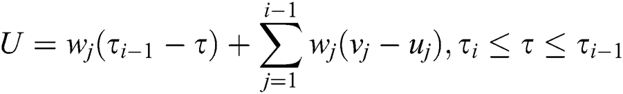
Here the per cycle cost of lead time crashing (U) is as follows
8. During the period of stock-out,  (ratio of backordering) is a variable and directly proportional to
  (per unit discount in backorder price, provided by supplier). So
  , where
  and
and  .
.
9. If the size of arrival lot is W with an imperfect rate s, then all products are identified and separated the imperfect products from the arrival lot W. So, the actual ordered quantity W is decreased by a quantity W(1 – s).
3 Mathematical Formulation of the Model
It is assumed that the lead time demand, i.e., Z has the probability distribution function  with mean
  and S.D
  . The per cycle expected counting of backorders is
  where
where  is the shortage against the expected demand after the cycle completion and
  is the annual cost of stock-out. The level of net inventory (expected) before the arrival of lot of order is
  . The total expected cost (annual) will consist of imperfect holding, non-imperfect holding cost, ordering cost, and inspection cost, the cost of lead time crashing and cost of stock-out. The combined inventory function of cost (TIC) is given as below

Here  is the number of expected orders annually.
In this study the ordering cost C is considered as a decision variable. The sum of capital investment cost and all inventory costs can be minimized by optimizing over W, C, R,  and
and  with the constraint
  , where
  is the actual cost of ordering. Now, the capital investment of supplier is
  , where
  is the per year opportunity capital cost (fractional annual) and obeys the logarithmic investment function defined as
  ,
,  , where 1/m is the fraction of decrement in C against the increment in investment (per dollar). Thus from Eq. (1)

Furthermore during the period of stock-out, the ratio of backorder ( ) is a variable and directly varies to the price discount in backorder (
 ) provided by the supplier (per unit). Thus
  , where
  and
and  . So the per unit price discount of backorder (
 ) is considered as a decision inconstant in place of ratio of backorder (
 ). So Eq. (2) will become

It is assumed that the demand of lead time Z abides normal distribution with p.d.f  , mean DL and S.D
  . We have
  , here j is safety factor and the shortage quantity (expected) at the completion of cycle is given as
  , where
  . Here
  is standard normal p.d.f and
  is cumulative distribution function. Hence Eq. (3) can be expressed as

For the solution of Eq. (4) we differentiae  partially with respect to W, C, j,
  and
and  respectively. We have


where  , x is standard normal variable.


By checking the sufficient conditions, for fixed  ,
,  is concave for
  as
as

So, for fixed  , the total expected minimum cost (annual) will exist at the last of the interval
  . Now, by putting Eq. (6) equal to zero and then solving for C, we have

Now, putting Eq. (6) equal to zero and then solving for  , we have

Putting the value of  from Eq. (12) in Eq. (5) and then putting it equal to zero, have

where 
Now, again putting the value of  from Eq. (12) in Eq. (7) and then setting it equal to zero, we have

To find the values of  , we solve the Eqs. (11) to (14) for the interval
  and denote these values by
  respectively. The following postulation claims that, for fixed interval
  the point
  is the optimal solution for the minimum expected annual cost.
Postulation 1. The Hessian matrix for  in interval
  is positive define at the point
  .
.
The effects of C on the total annual cost (expected) can be examined by finding the partial derivative of second order of  with respect to C and obtaining
  . Thus
  is convex in C for fixed
  and
and  . Since it is not easy to find the solution for
 , so the following algorithm is used to find the solution
Algorithm 1
Step 1. For every  (i = 0,1, 2, 3…n) perform the following sub steps
(i) Start with  and
and 
(ii) Evaluate  by substituting
  and
and 
(iii) With this value of  find
find  by Eq. (11),
  by Eq. (12) and
  by Eq. (14)
(iv) Determine  and then
(v) Repeat sub steps (ii) to (iv) until the values of  and
and  are unchanged.
Step 2. Compare  with
with  and
and  with
with  , there will be two cases
(i) If  and
and  then
then  and
and  are feasible. Go to Step 3.
(ii) If  and
and  then
then  and
and  are infeasible. For a particular
  , let
, let  and
and  and find the values of
  by iterative methods with the help of Eqs. (12), (13) and (14). Go to Step 3.
Step 3. For every  determine the corresponding total expected cost (annual) by
  using Eq. (4).
Step 4.  and put
  = M. Then
  is the final solution and the optimal reordering point
  can be determined.
3.2 Model without Distribution
In real situations the distribution of probability for the demand of lead time is restricted. A good manager can predict the variance and mean value of the demand of lead time. The actual distribution of probability may not be known. Due to the absence of required things the anticipated shortage  is not known and so
  cannot be determined. To defeat this situation, assumption of normal distribution is moderated and assumed that the demand of lead time Z considered with first two moments. For instance the p.d.f
  of Z comes from the class
  with mean DL and S.D
  . Thus the procedure of minmax distribution-free is used to resolve this problem i.e., to determine the best p.d.f
  in
in  for every
  and the total expected cost can be minimized.
To find Min-Max  , the following preposition is required which was presented by Gallego et al. [6]

Substituting 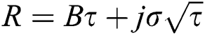 in (15), we have

Now using Eq. (3) and inequality (16) and taking the factor of safety j as a decision v factor in place of R, the function of can be presented as
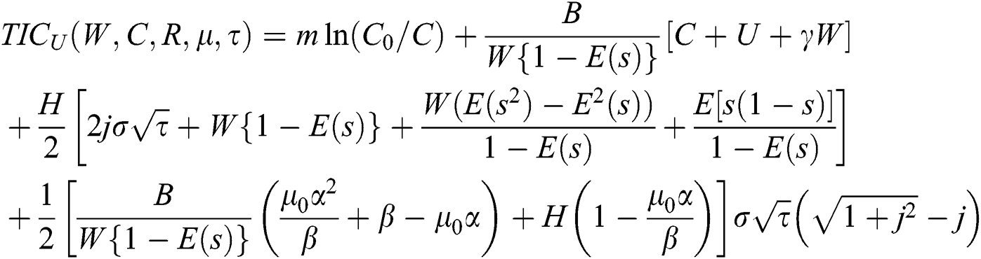
Here  is the t final expected cost for distribution-free and it is the supremum of
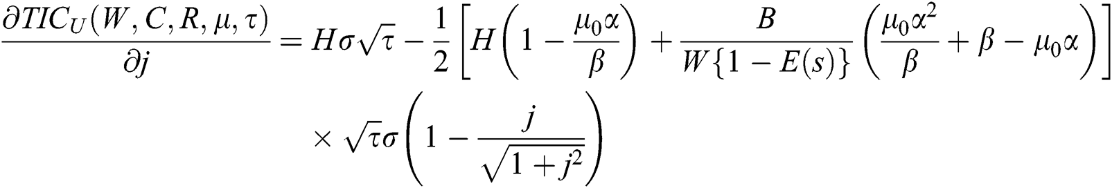
  . Now we differentiate Eq. (17) with respect to W, C, R,
  and
and  respectively in the interval
  , we have


By checking the second order partial derivative, the sufficient conditions, for fixed  ,
,  is concave in the interval
  as
as

So, for fixed  , the total expected minimum cost (annual) will exist at the last of the interval
  . Now, by putting Eq. (19) equal to zero and then solving for C, we have

Similarly solving for  by putting Eq. (21) to zero, we have

Again putting Eq. (25) into Eq. (18) and then putting it to zero, we have

where 
Now, putting Eq. (25) into Eq. (20) and then putting it to zero, we have

To find the values of  , we solve the Eqs. (24) to (27) for the interval
  and denote these values by respectively (we represent these terms by
  ). The following postulation claims that, for fixed interval
  , the point
  is the optimal solution for the minimum expected annual cost.
Postulation 3. The Hessian matrix for  in interval
  is positive define at the point
  .
.
The effects of C on the total annual cost (expected) can be examined by finding the partial derivative of second order of  with respect to C and obtaining
  .
.
Thus  is convex in C for fixed
  and
and  . Since it is not easy to find the solution for
  , so the Algorithm 2 is executed to determine the solution of
  represented by
  .
.
Algorithm 2
Step 1. For every  (i = 0,1, 2, 3, …, n) perform the following sub steps
(i) Start with  and
and 
(ii) Evaluate  by substituting
  in Eq. (26)
(iii) With this value of  find
find  by Eq. (24),
  by Eq. (25) and
  by Eq. (27)
(v) Repeat sub steps (ii) to (iii) until the values of  and
and  are unchanged.
Step 2. Compare  with
with  and
and  with
with  , there will be two cases
(i) If  and
and  then
then  and
and  are feasible. Go to Step 3.
(ii) If  and
and  then
then  and
and  are infeasible. For a particular
  , let
, let  and
and  and find the values of
  by iterative methods with the help of Eqs. (26), (27) and (25). Go to Step 3.
Step 3. For every  determine the corresponding total expected cost (annual) by
  using Eq. (17).
Step 4.  and put
  = M. Then
  is the solution and the reorder point
  can be obtained.
4 Numerical Verification of the Study
To verify the present study and illustrate the effects of reduction in ordering cost, an inventory product is considered with the same parameter values as in Pan et al. [16]. B = 600 units (every year), H = 20$/unit/year,  = 200$/order,
  = 12$/unit/year,
  = 7 units/week,
  = 150$/unit lost,
  = 1.6$/unit. For the reduction in ordering cost, we consider
  = 0.1 and m = 5800. There are three components of lead time
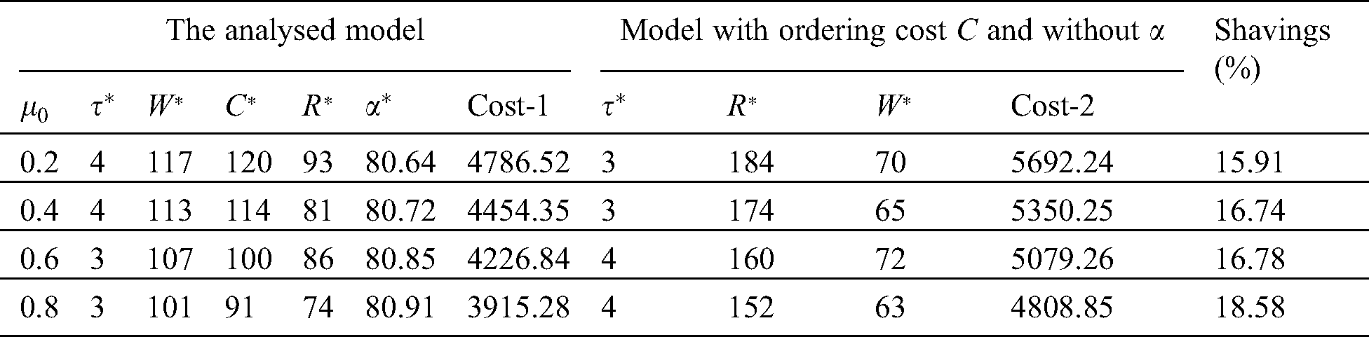
Example 1. Suppose a normal distribution follows the demand for lead time. The results are presented in Tab. 1 and Tab. 2 for = 0.2, 0.4, 0.6, 0.8 by using the Algorithm 1. Next, an analysis of optimal solutions is presented in Tab. 3 and to observe the impacts of reduction in the cost of ordering and discount in backorder price. The same Tab. 3 includes the results with the fixed cost of ordering and with no discount on the backorder price. The shavings can be observed by comparing both the cases, which range between 18.52% to 21.45%.
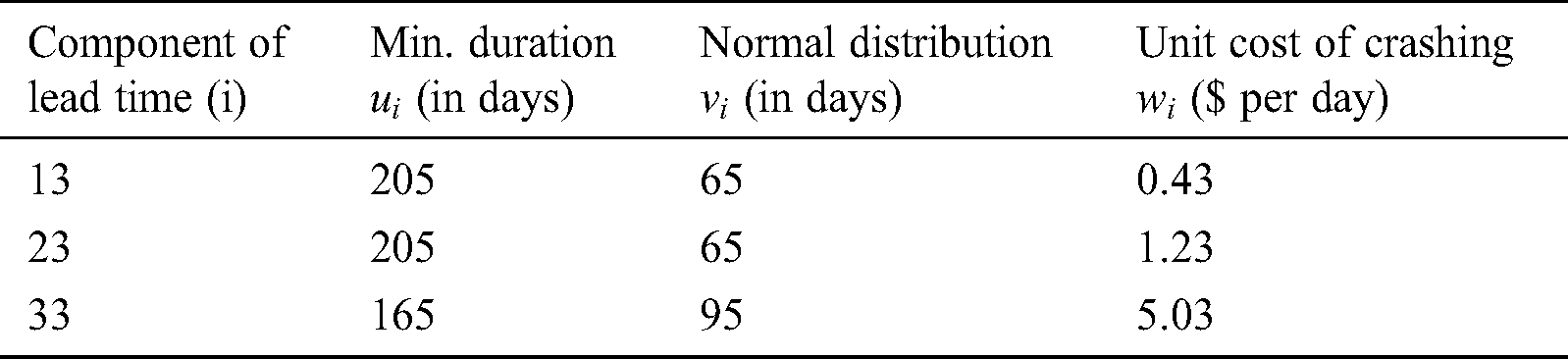
Table 2: Solution process for Example 1 ( in weeks)
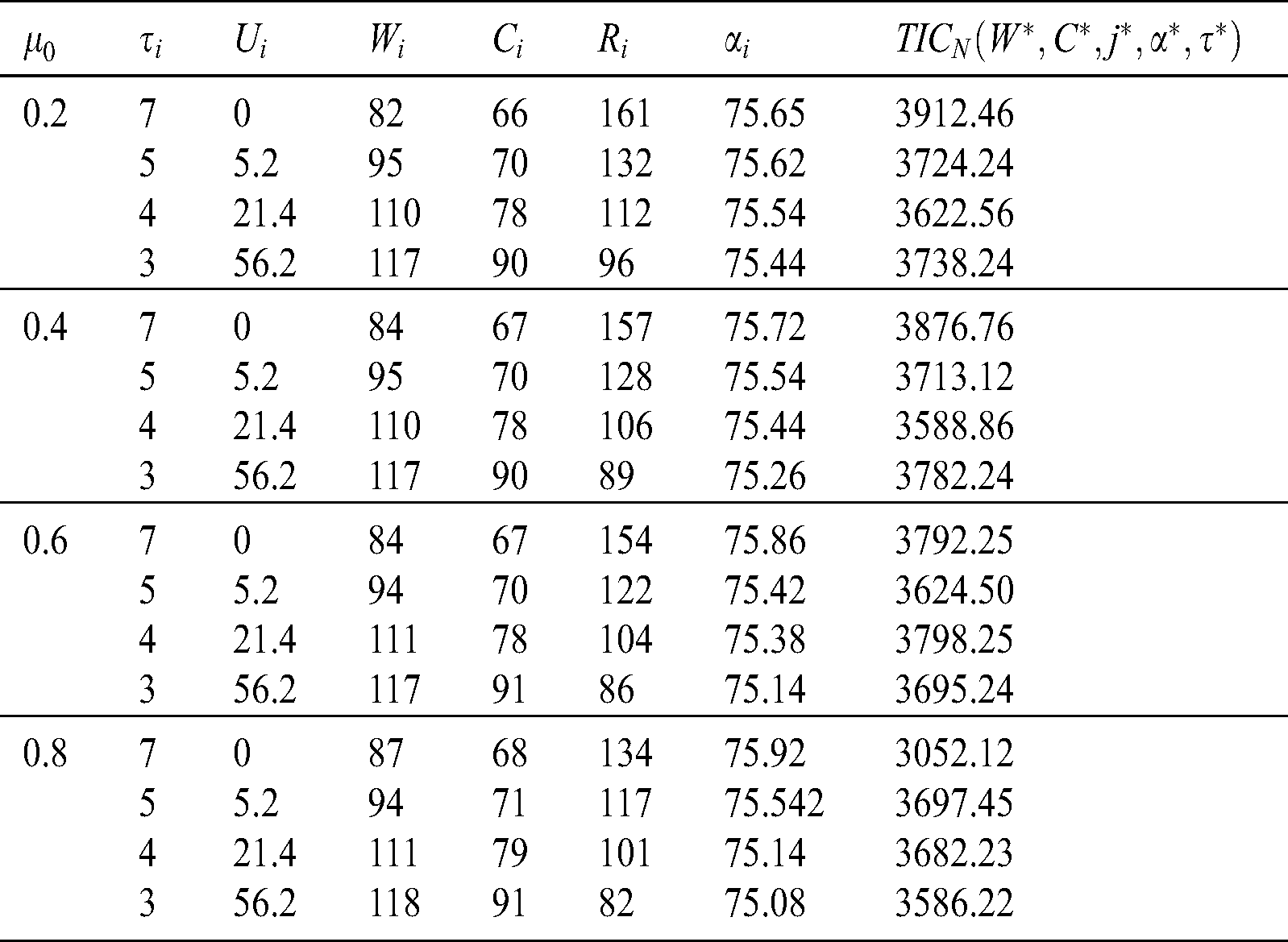
Table 3: Summarized optimal solution for Example 1 ( in weeks)
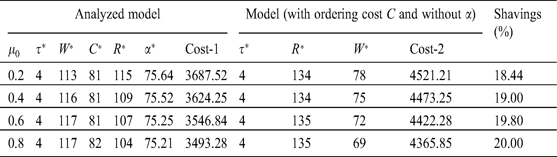
Example 2. In this example the data of Example 1 is considered except the condition that distribution of probability of the demand of lead time is not known. Using the Algorithm 2, find the results presented in Tab. 4 and Tab. 5 includes the analyzed optimal values. The comparative results of Tab. 5 reflect that in case of bad distribution of demand of lead time, it is preferable to invest in reduction of ordering cost and permit discount in price of backorder to resolve the problem of ordering during the period of shortages. The shavings can be observed by comparing both the cases, which range between 18.44% to 20%.
Table 4: Solution process for Example 2 ( in weeks)
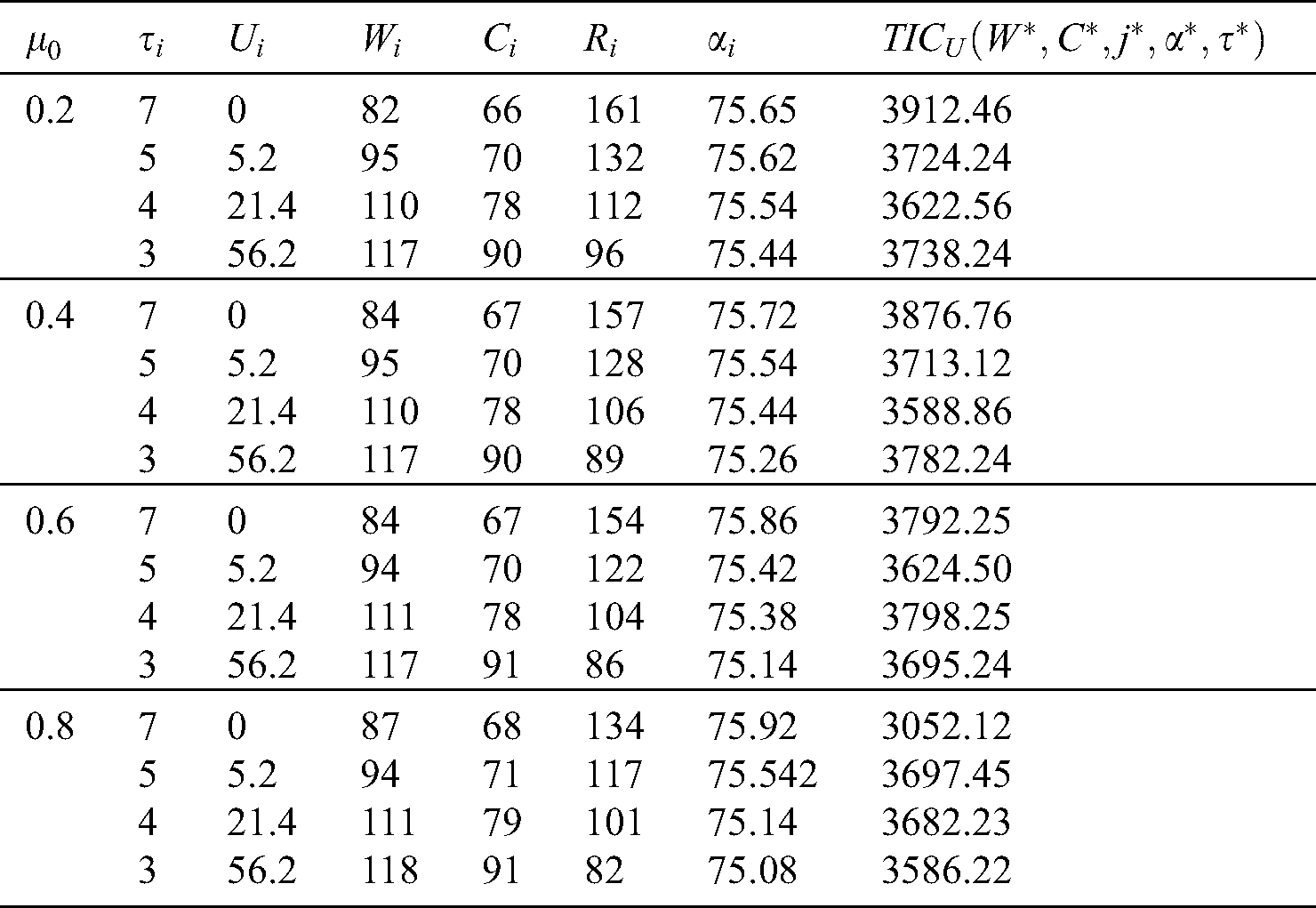
Table 5: Summarized optimal solution for Example 2 ( in weeks)
With the help of these two examples, it can be observed that the shavings of total expected cost (annual) are examined by the reduction in ordering cost and discount in price of backorder’. Next, we test the importance of distribution-free concept in comparison of normal distribution. If we use the solution in place of  , then
  will be the added cost.
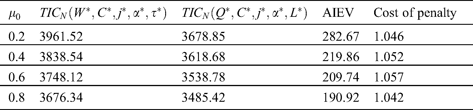
This is hugest quantity for the information p.d.f  and the amount is assumed as the additional information of expected value (AIEV) and its précis is shown in Tab. 6. In practice, the model (Reduction in ordering cost) with the discount in backorder price is more like the supply chain of real life.
Table 6: Determination of additional information of expected value (AIEV)
The occurrence of unsatisfied demands increases the period of lead time and decreases the backorders in the same ratio. In the case of probabilistic needs, the shortages cannot be ignored. To solve this type of problem and to cover the losses of customers, a discount in backorders may be offered by the supplier. Also, our inventory policies may not be good for the arriving lots, which include some imperfect products. This study aims to check the impact of imperfect products on a unified policy by permitting the discount in the price of backorders and considering the cost of ordering as decision factors. First, it is assumed that the demand for lead time is followed by a normal distribution and then stops it and assumed that the first two moments of demand for lead time are known. Further, the minimax distribution method is used to solve this model, and a separate algorithm is designed. Since the situations of markets are regularly changing, so the policies of corporate should be managed suitably. If it is possible to decrease the cost of ordering correctly and the orders fixed well, the per unit time total concern cost will be upgraded. On the other side, if the seller provides a better discount in the backorder to the purchaser, then the service level will be improved, and the total expected cost (annual) will be reduced. This study covers the above literature gaps and is supported by numerical verification.
By the examples, it is observed that a notable quantity of shavings can be attained. It also reflects the suggestions to invest only when there is a chance of improvement. Computed results tell us the significant effects of weak quality of supply on the related cost and parameter sensitivity. This study provides an application in inventory models involving inspections, ordering quantity, and imperfect products. The presented research further is suitable for more general inventory characteristics in various real-life problems.
Funding Statement: The author(s) received no specific funding for this study. The Graphic Era Hill University Dehradun supported the research of the Sandeep Kumar and Teekam Singh. The corresponding and the third authors thank Prince Sultan University for the financial support.
Conflicts of Interest: The authors declare that they have no conflicts of interest to report regarding the present study.
1. J. A. Buzacott. (1975). “Economic order quantity with inflation,” Operational Research Quarterly, vol. 26, no. 3, pp. 553–558. [Google Scholar]
2. R. B. Misra. (1979). “A note on optimal inventory management under inflation,” Naval Research Logistics Quarterly, vol. 26, no. 1, pp. 161–165. [Google Scholar]
3. J. K. Dey, S. K. Mondal and M. Matti. (2008). “Two shortage inventory problem with dynamic demand and interval valued lead time over finite time horizon under inflation and time-value of money,” European Journal of Operational Research, vol. 185, no. 1, pp. 170–194.
4. F. Jolai, R. T. Moghaddam, M. Rabbani and M. R. Sadoughian. (2006). “An economic production lot size model with deteriorating items, stock-dependent demand, inflation, and partial backlogging,” Applied Mathematics and Computation, vol. 181, no. 1, pp. 380–389. [Google Scholar]
5. S. K. Goyal. (1984). “Economic ordering policy for a product with periodic price changes,” in Proc. of Third Int. Symp. on Inventories, Budapest, Hungry. [Google Scholar]
6. K. S. Park. (1986). “Inflationary effect on EOQ under trade-credit financing,” International Journal on Policy and Information, vol. 10, no. 2, pp. 65–69. [Google Scholar]
7. P. Vrat and G. Padamanabban. (1990). “An inventory model under inflation for stock dependent consumption rate items,” Engineering Costs and Production Economics, vol. 19, no. 1–3, pp. 379–383. [Google Scholar]
8. T. K. Datta and A. K. Pal. (1991). “Effects of inflation and time value of money on an inventory model with linear time-dependent demand rate and shortages,” European Journal of Operational Research, vol. 52, no. 3, pp. 326–333. [Google Scholar]
9. C. J. Liao and C. H. Shyu. (1991). “An analytical determination of lead time with normal demand,” International Journal of Operations and Production Management, vol. 11, no. 9, pp. 72–78. [Google Scholar]
10. M. Ben-Daya and A. Raouf. (1994). “Inventory models involving lead time as a decision variable,” Journal of the Operational Research Society, vol. 45, no. 5, pp. 579–582. [Google Scholar]
11. L. Y. Ouyang and B. R. Chuang. (2000). “A periodic review inventory model involving variable lead time with a service level constraint,” International Journal of System Science, vol. 31, no. 10, pp. 1209–1215. [Google Scholar]
12. L. Y. Ouyang, K. S. Wu and C. H. Ho. (2007). “An integrated vendor-buyer inventory model with quality improvement and lead time reduction,” International Journal of Production Economics, vol. 108, no. 1–2, pp. 349–358. [Google Scholar]
13. M. A. Hoque and S. K. Goyal. (2009). “An alternative simple solution algorithm of an inventory model with fixed and variable lead time crash costs under unknown demand distribution,” International Journal of Systems Science, vol. 40, no. 8, pp. 821–827. [Google Scholar]
14. W. C. Lee. (2005). “Inventory model involving controllable backorder rate and variable lead time demand with the mixtures of distribution,” Applied Mathematics and Computation, vol. 160, no. 3, pp. 701–717. [Google Scholar]
15. G. Gallego and I. Moon. (1993). “The distribution free newsboy problem: Review and extensions,” Journal of Operational Research Society, vol. 44, no. 8, pp. 825–834. [Google Scholar]
16. J. C. H. Pan and Y. C. Hsiao. (2005). “Integrated inventory models with controllable lead time and backorder discount considerations,” International Journal of Production Economics, vol. 94, no. 4, pp. 387–397. [Google Scholar]
17. W. C. Lee, J. W. Wu and C. L. Lei. (2007). “Computational algorithm procedure for optimal inventory policy involving ordering cost reduction and back-order discounts when lead time demand is controllable,” Applied Mathematics and Computation, vol. 189, no. 1, pp. 186–200. [Google Scholar]
18. M. K. Salameh and M. Y. Jaber. (2000). “Economic production quantity model for items with imperfect quality,” International Journal of Production Economics, vol. 64, no. 1–3, pp. 59–64. [Google Scholar]
19. M. Y. Jaber, S. K. Goyal and M. Imran. (2008). “Economic production quantity model for items with imperfect quality subject to learning effects,” International Journal of Production Economics, vol. 115, no. 1, pp. 143–150. [Google Scholar]
20. H. C. Chang and C. H. Ho. (2010). “Exact closed form solutions for optimal inventory model for items with imperfect quality and shortage backordering,” Omega, vol. 38, no. 3–4, pp. 233–237. [Google Scholar]
21. P. A. Hayek and M. K. Salameh. (2001). “Production lot sizing with the reworking of imperfect quality items produced,” Production Planning & Control, vol. 12, no. 1, pp. 584–590. [Google Scholar]
22. K. Annadurai and R. Uyhayakumar. (2010). “Controlling set-up cost in (Q, r, L) inventory models with defective items,” Applied Mathematical Modeling, vol. 34, no. 6, pp. 1418–1427. [Google Scholar]
23. R. L. Schwaller. (1988). “EOQ under inspection costs,” Production and Inventory Management Journal, vol. 29, no. 3, pp. 22–29. [Google Scholar]
24. M. K. Salmeh and M. Y. Jaber. (2000). “Economic production quantity model for items with imperfect quality,” International Journal of Production Economics, vol. 64, no. 1–3, pp. 59–64. [Google Scholar]
25. H. C. Chang. (2004). “An application of fuzzy sets theory to the EOQ model with imperfect quality items,” Computer & Operation Research, vol. 31, no. 12, pp. 2079–2092. [Google Scholar]
26. M. J. Paknejad, F. Nasri and J. F. Affiso. (1995). “Defective units in a continuous review system,” International Journal of Production Research, vol. 33, no. 10, pp. 2767–2777. [Google Scholar]
27. B. Sarkar, S. S. Sana and K. Chaudhuri. (2011). “An economic production quantity model with stochastic demand in an imperfect production system,” International Journal of Services and Operations Management, vol. 9, no. 3, pp. 259–283. [Google Scholar]
28. K. J. Chung, C. C. Her and S. D. Lin. (2009). “A two-warehouse inventory model with imperfect quality production processes,” Computers & Industrial Engineering, vol. 56, no. 1, pp. 193–197. [Google Scholar]
29. S. Papachristos and I. Konstantaras. (2006). “Economic ordering quantity models for items with imperfect quality,” International Journal of Production Economics, vol. 100, no. 1, pp. 148–154. [Google Scholar]
30. A. Eroglu and G. Ozdemir. (2007). “An economic order quantity model with defective items and shortages,” International Journal of Production Economics, vol. 106, no. 2, pp. 544–549. [Google Scholar]
31. H. Wee, J. Yu and M. Chen. (2007). “Optimal inventory model for items with imperfect quality and shortage backordering,” Omega, vol. 35, no. 1, pp. 7–11. [Google Scholar]
32. M. Khan, M. Y. Jaber, A. L. Guiffrida and S. Zolfaghari. (2011). “A review of the extensions of a modified EOQ model for imperfect quality iteming,” International Journal of Production Economics, vol. 132, no. 1, pp. 1–12. [Google Scholar]
33. S. K. Goyal and L. E. Cardenas-Barron. (2002). “Note on economic production quantity model for items with imperfect quality—A practical approach,” International Journal of Production Economics, vol. 77, no. 1, pp. 85–87. [Google Scholar]
34. W. M. Chan, R. N. Ibrahim and P. B. Lochert. (2003). “A new EPQ model: Integrating lower pricing, rework and reject situations,” Production Planning & Control, vol. 14, no. 7, pp. 588–595. [Google Scholar]
35. W. C. Lee, J. W. Wu, H. H. Tsou and C. L. Lei. (2012). “Computational procedure of optimal inventory model involving controllable backorder rate and variable lead time with defective units,” International Journal of Systems Science, vol. 43, no. 10, pp. 1927–1942. [Google Scholar]
36. K. Skouri, I. Konstantaras, A. G. Lagodimos and S. Papachristos. (2014). “An EOQ model with backorders and rejection of defective supply batches,” International Journal of Production Economics, vol. 155, no. 1, pp. 148–154. [Google Scholar]
 | This work is licensed under a Creative Commons Attribution 4.0 International License, which permits unrestricted use, distribution, and reproduction in any medium, provided the original work is properly cited. |