DOI:10.32604/cmc.2021.014509
| Computers, Materials & Continua DOI:10.32604/cmc.2021.014509 | |
| Article |
Estimating Loss Given Default Based on Beta Regression
1Department of Risk Management and Insurance, The University of Jordan, Aqaba, 77111, Jordan
2Universiti Kebangsaan Malaysia, Department of Mathematical Sciences, Malaysia
3Department of Basic Sciences, College of Science and Theoretical Studies, Saudi Electronic University, Riyadh, 11673, Saudi Arabia
*Corresponding Author: Nawaf N. Hamadneh. Email: nwwaf977@gmail.com
Received: 24 September 2020; Accepted: 19 October 2020
Abstract: Loss given default (LGD) is a key parameter in credit risk management to calculate the required regulatory minimum capital. The internal ratings-based (IRB) approach under the Basel II allows institutions to determine the loss given default (LGD) on their own. In this study, we have estimated LGD for a credit portfolio data by using beta regression with precision parameter ( ) and mean parameter
  . The credit portfolio data was obtained from a banking institution in Jordan; for the period of January 2010 until December 2014. In the first stage, we have used the “outstanding amount” and “amount of borrowing” to find LGD of each default borrower (494 out of 4393 borrower). In the second stage, we fit univariate parametric distributions to the LGD data to obtain the beta distribution. After that, we have estimated the values of
  based on microeconomic variables (SPP, OE and LR). Moreover, we have estimated the values of
  based on macroeconomic variables (GDP and Inflation rate). Finally, we have compared between six different link functions (Logit, loglog, probit, cloglog, cauchit, and log), which have used with
  and
and  . The results show that Beta regression with probit link function has the highest R-squared with accepted measurements for logL, AIC and BIC.
Keywords: Credit risk; loss given default; parametric distribution; regression model
The Basel Committee gives three approaches to estimate the required regulatory capital in banking institutions; standardized, internal ratings-based (IRB) and progressing IRB. The IRB approach is generally favored compared to the standard approach because it produces higher accuracy estimates and lower capital charges. The IRB approach under the Basel II allows institutions to determine probabilities of default (PD) and loss given default (LGD) on their own, as opposed to the standardized approach under the Basel I which uses estimates of PD and LGD from the Central Bank to calculate the required capital based on a percentage of risk-weighted-assets. Thus, the Basel II leads to a better differentiation of risks and considers diversification of a bank’s portfolio [1,2].
In Jordan, the banking sector obtains the estimate of LGD from the Central Bank of Jordan under the Basel I. Therefore, the LGD estimate is fixed, and does not varies according to banks. The contributions of this chapter are to estimate the LGD under the Basel II for corporate credit portfolio in the Jordanian banking sector, to fit the LGD data to parametric distributions, and to incorporate internal and external financial variables into the data so that the LGD data can be fitted to regression models. The main advantage of fitting the LGD data with financial variables as covariates is that we can determine which financial variables significantly affect the LGD. Since the LGD is influenced by some key transaction characteristics, several categories of variables such as macroeconomic and industry-specific variables can be used to build a predictive regression model.
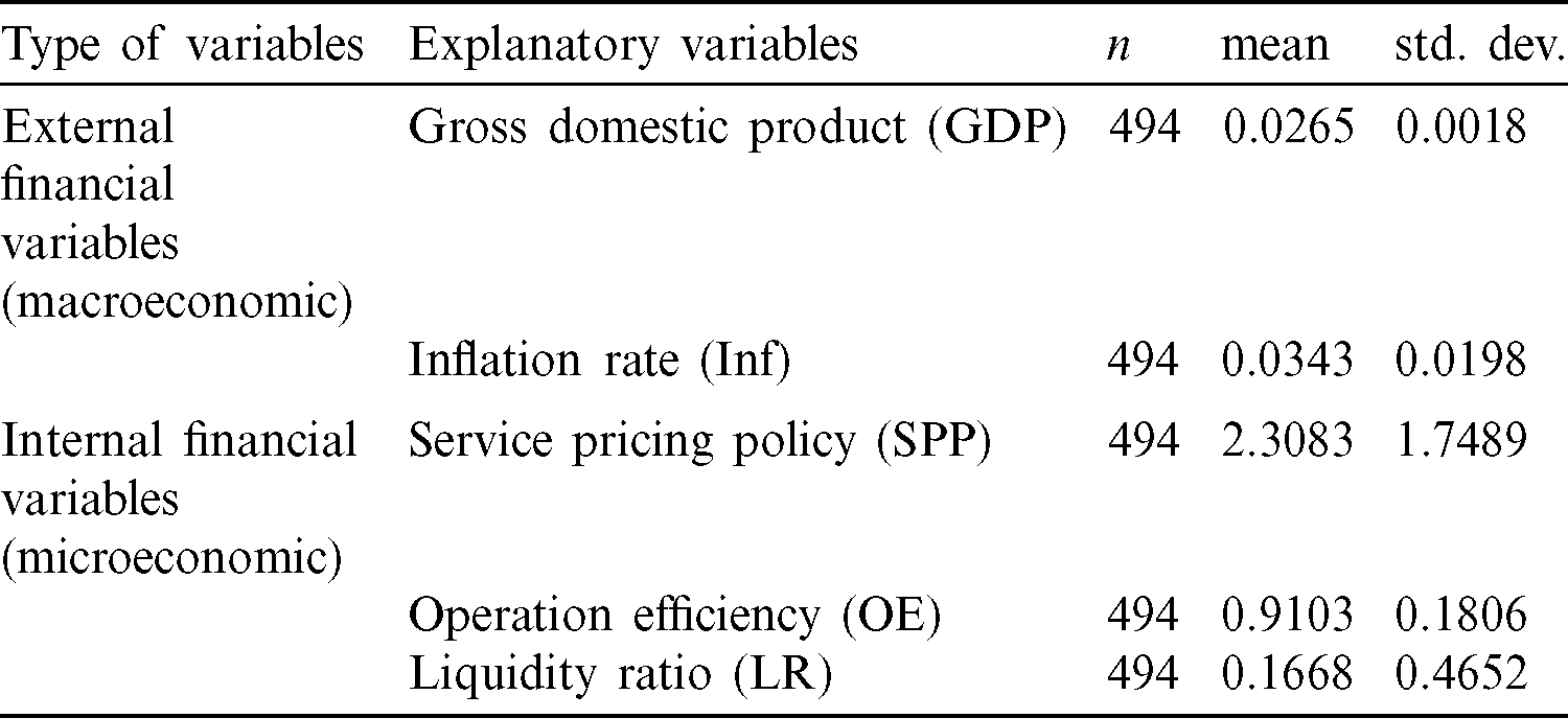
The objective of this chapter is to use several parametric models (beta, Cauchy, gamma, Gompertz, logistic, log-normal, gamma, normal, and Weibull) to estimate LGD. The models are fitted to a sample data obtained from the corporate credit portfolio of a bank in Jordan for the period of January 2010 until December 2014. The LGD data lies between interval [0,1] because it is the proportion of outstanding amount from the borrowing amount. We also consider five financial variables for the regression model to determine the financial variables, which significantly affect the LGD. The financial variables are gross domestic product (GDP), inflation rate (Inf), service pricing policy (SPP), operating efficiency (OE), and liquidity ratio (LR).
The rest of this paper proceeds as follows. In the next section, we discuss the literature review for important work for LGD, and Section 3 describes the parametric distributions for fitting the LGD data and the regression models for determining the financial variables which significantly affect the LGD. We present the sample data and the empirical results in Section 4, and the final section concludes.
Most empirical studies on credit risk depended heavily on corporate bond markets to gauge losses in the case of default. The reason behind this is that bank loans are private instruments, and thus, little information on loan losses are freely accessible. Several studies on credit risks and LGD on bond markets have been carried out in the last several decades. An earlier study can be found in [3] who utilized actuarial analysis to investigate mortality rates of U.S. corporate bonds. This was followed by various empirical studies on credit risk in bond markets (see, for example [4,5]). The mortality approach was also used by [6] to measure the percentage of bad and doubtful loans of corporate bond recovered several months after the default date. Recent studies on LGD can be found in [7] who proposed a new model for LGD of bank loans by leveraging time to recovery, and reference [8] who forecasted LGD of bank loans using multi-stage model. In another study, [9] constructed a survival model to predict risks of cardholders and applied the model to a case study in Capital Card Services.
LGD data from banking industry tends to be skewed and heavy-tailed, and thus, can be fitted by parametric models such as beta, lognormal, gamma, and Pareto. Besides parametric models, non-parametric models were also proposed and used, such as regression tree, neural networks, multivariate adaptive regression spline, and least squares support vector machine [10–17].
For the case of LGD with covariates, regression models can be utilized and several examples can be found from past studies. Examples of regression models for LGD data are ordinary least squares regression (OLS), ridge regression (RiR), and fractional response regression. In 2005 Moody’s introduced the renowned LossCals Model using a multivariate linear regression model consisting of industry and macroeconomic factors, and reference [18] applied logistic regression with time consideration using transformed LGD as dependent variable and macroeconomic variables as independent variables. Recently, reference [19] used quintiles regression to estimate downturn and unexpected credit losses known as downturn LGD. Finally, reference [9] constructed a model to predict the risk of a cardholder for the lifetime of account and applied survival analysis methodologies to a case study in capital card services.
Under the Basel II, banking institutions are suggested to consider macroeconomic downturn conditions when estimating recovery rates [20–22]. In particular, reference [22] assumes that banking institutions should use gross domestic product (GDP) growth rate and unemployment rate as determinants of recovery rate prediction. It should be noted that recovery rate is equal to one minus LGD rate. Studies from [23,24] showed that GDP growth rate was significantly relevant to the recovery rate of the U.S. bonds. On the other hand, references [12,25] found that GDP growth rate was not significantly relevant.
Other macroeconomic covariates were also suggested in the literature to predict recovery rate, such as inflation rate [24], interest rate [14,24], growth rate of investment [12,26] and rate of return on stock market [24,25]. Studies from [6,27] showed that recovery rate decreases when loan size increases. In another study, reference [8] used Japanese credit portfolio to analyze impacting factors of LGD and to improve multi-stage model for predicting LGD. The variables considered are creditworthiness score, collateral quota (commercial bills), collateral quota (real estate), collateral quota (marketable securities), collateral quota (deposits), credit guarantee quota, and exposure (in hundred million yen). Their results showed that collateral, guarantees, and loan size significantly affect the LGD.
In this study, we consider macro- and micro-economics factors as explanatory variables, and the factors are obtained from available reports. We use macro-economic factors (GDP and inflation rate) for the mean parameter and micro-economic factors (service pricing policy, operating efficiency, and liquidity ratio) for the dispersion parameter in beta regression model.
3 Methodology for Estimating LGD
This section gives a background of the main concepts used in our study. Our model consists of three stages. In the first stage, we use the outstanding amount and amount of borrowing to find LGD of each default borrower. In the second stage, we will use the LGD to find the suitable parametric model. In the third stage, we will use beta regression with different link functions for fitting the LGD data with covariates for two parameters for beta regression.
A variety of models in which LGD is subject to systematic risk can be found in the literature. Reference [28] proposed a model in which the LGD is normally distributed and influenced by the same systematic factor that drives the probability of default (PD). Reference [10] employs a lognormal distribution for the LGD. Other extensions include [29], choosing a probit transformation. References [30,31] employ a logit transformation. However, reference [6] used mortality approach to measure the percentage of bad and doubtful loan of corporate bonds that are recovered n months after the default date. The actuarial-based mortality approach is appropriate because the population sample is changing over time. The dataset of this study is obtained from micro-data on defaulted bank loans of a private bank in Portugal, Banco Commercial Portugues (BCP). It consists of 10000 short-term loans granted to small and medium-sized companies from June 1995–December 2000 (66 months). They identified the LGD by the following:  ,
,  , and
, and  where
where  is a sample (weighted) percentage of unpaid loan balance at period
  ,
,  is a sample (weighted) marginal recovery rate at time
  ,
,  refers to each of the
  loan balances outstanding in the sample, and
  is the periods after default. They found that the cumulative average recovery is almost completed after 48 months. Moreover, the distribution of cumulative recovery rates is a bi-model distribution. Reference [32] used unsecured consumer loans or credit cards for one UK lender to compare linear regression and survival analysis models to predict LGD. The datasets were collected on 27000 personal loans from 1989–2004. There are two reasons to use survival analysis. Firstly, debts which are still being repaid cannot be included in the standard linear regression approach. Survival analysis models can treat such repayments as censored and easily include them in the model. Secondly, the recovery rate is not normally distributed and therefore modeling it using a linear regression violates the assumptions of linear regression models. The recovery rate is defined as:
  , where RR is a recovery rate and
  . The study compared linear regression with survival analysis models (proportional hazard models and accelerated failure time models for Weibull, log–logistic, gamma, and Cox model). The linear regression is better than survival models in single distribution models based on higher R-square, higher Spearman rank, and lower MSE. Reference [6] used LGD ratio as shown before to estimate the percentage of LGD after n-months of corporate bond default. However, reference [32] considered equation as shown before to estimate LGD ratio for personal loans. Our study constructs LGD ratio from previous equations to estimate LGD as shown in Eq. (1).

The Basel II risk parameters are PD, LGD and exposure at default (EAD). The rate of expected credit loss (ECL) which is also known as the risk-weighted-asset of credit portfolio can be expressed as the product of PD and LGD. Therefore, LGD is one of the two determining factors of credit losses [33]. The ECL of credit portfolio can generally be represented as:

where  is the probability of default of the ith borrower,
  is the loss given default,
  is the exposure at default, and m is the total number of borrowers in the portfolio.
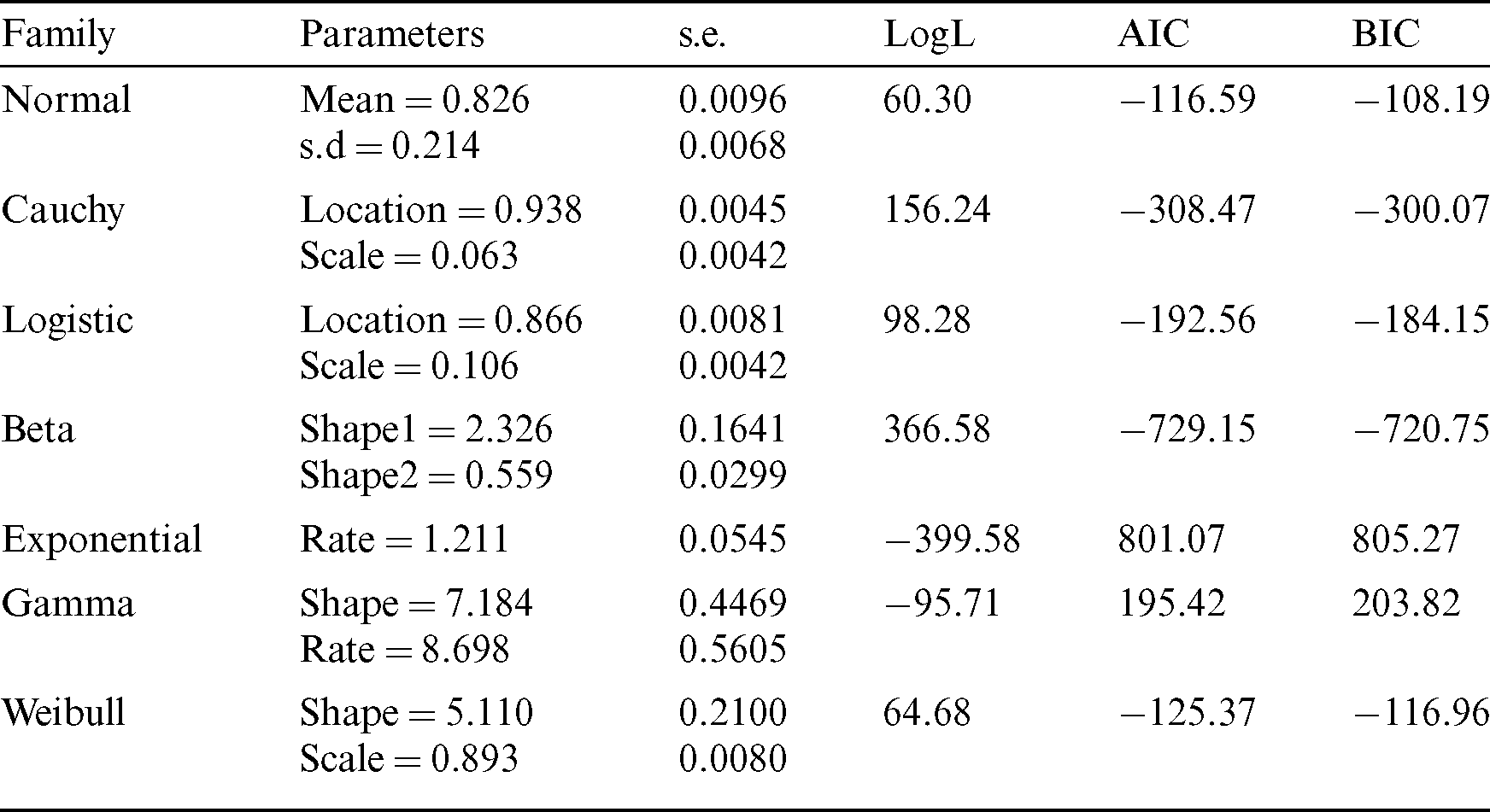
Common parametric distributions for modeling the LGD data are considered. Tab. 1 provides the density function and survival function for the distributions considered in this study, which are Beta, Cauchy, Gamma, Gompertz, Logistic, Log-normal, Normal, and Weibull. These distributions are suitable for modeling skewed and heavy-tailed data, which are commonly displayed in LGD data. The empirical pdf for the LGD data in our study can be seen in Fig. 1 (pdf). The curve of empirical pdf indicates that the LGD data is skewed and heavy-tailed.
Table 1: Parametric models for LGD

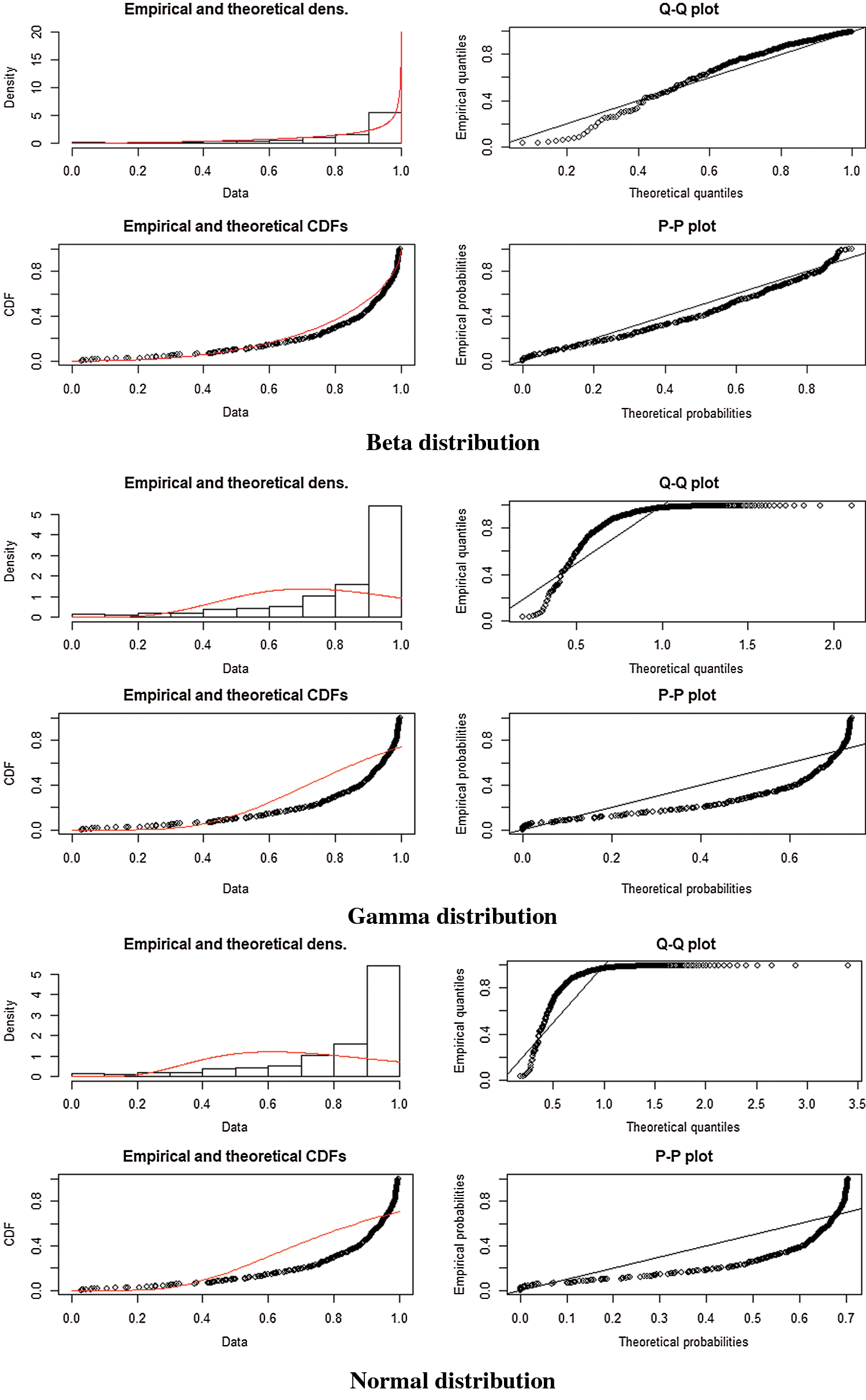
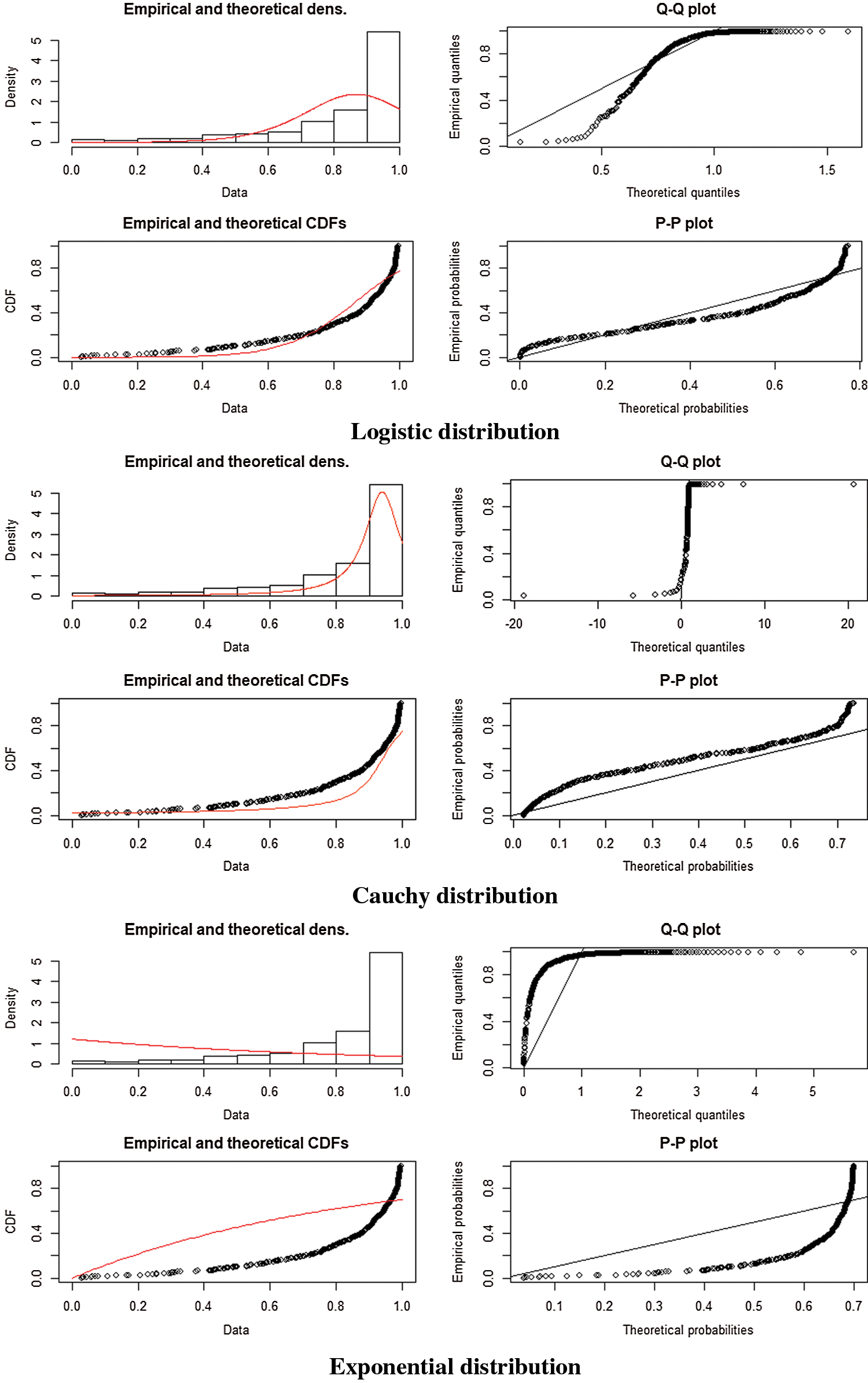
Figure 1: q–q plot, p–p plot, PDF and CDF. Beta distribution, gamma distribution, normal distribution, logistic distribution, Cauchy distribution, exponential distribution
Three types of accuracy criteria are used to choose the best model; Akaike information criterion (AIC), Bayesian information criterion (BIC), and Log-likelihood (LogL). BIC is depend on maximum likelihood estimates of the model parameters [34], which penalizes a sample data with larger size and number of parameters. The formula is defined as  where
where  refers to the log likelihood of the estimated model, p refers to the number of parameters, and
  . AIC is also depend on maximum likelihood estimates of model parameters [35], but penalizes a sample data with larger size. The formula is defined as
  where
where  refers to the log likelihood of the estimated model, p refers to the number of parameters, and k * = 2 .
In our study we use beta regression for fitting the LGD data with covariates. The reason for fitting beta regression is that the distribution is well common to be adequate for modeling quantities bounded in the interval [0,1]. Based on the selection of parameters, the probability density function can be unimodal, J-shaped, U-shaped or uniform. It can be shown in the later section that beta distribution is the best model compared to other parametric distributions for fitting the sample data without covariates for our case study. Therefore, we consider several beta regressions, by using different link functions, for fitting the LGD data with covariates.
Let random variable  follows to Beta distribution,
  , where the parameters are
  . The mean and variance of
  are defined as
  and
and  respectively. Reference [36] defined a regression structure of beta distribution as the followings. Let
  and
and  so that
  and
and  . The new parameterizations of Beta regression are
  and
and  , where
  for
for  with
with  and
and  since
since  . Parameter
  is known as precision parameter. Since a larger
  indicates as smaller variance for a fixed
  ,
,  can also be regarded as the dispersion parameter.
In our study, the precision parameter is modeled in a similar way as the mean parameter. Instead of having a fixed dispersion (fixed variance) we have a varying dispersion (varying variance). Therefore, a varying variance indicate a varying risks and it would be beneficial if significant risk factors (significant covariates) can be determined. It should be noted that variance is commonly used as one of the risk measures in finance area. The risk of loss in finance can be measured using confidence interval, for instance, the 95% confidence interval for loss can be measured as  , where
  is the standard deviation.
Let  be a random samplewhere
  ,
,  . The parameters,
  and
and  , are assumed to satisfy the following functional relations:
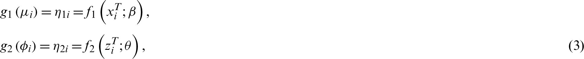
where  and
and  are defined as vectors of unknown regression parameters that are assumed to be functionally independent,
  and
and  ,
,  are predictors, and
  ,
,  are observations on q1 and q2 known covariates which need not be exclusive.
A number of several link functions can be used for g(.), such as logit specification which defined as  , probit function
  where
where  refer to the standard normal distribution function, log function
  , complementary log–log function
  , and Cauchy function
  . A rich discussion on the link functions can be explained in [37,38], or by referring to Chapter 7 in [39].
The log-likelihood function of Beta regression models defined as:

where  , and
, and  and
and  are functions of
  as defined in Eq. (3), respectively. The estimated parameters can be derived by maximizing the likelihood in (4). Further details on Beta regression can be found in [40].
In this study, we consider Beta regression with different link functions for fitting LGD data with covariates. We use R-squared to select the best regression model.
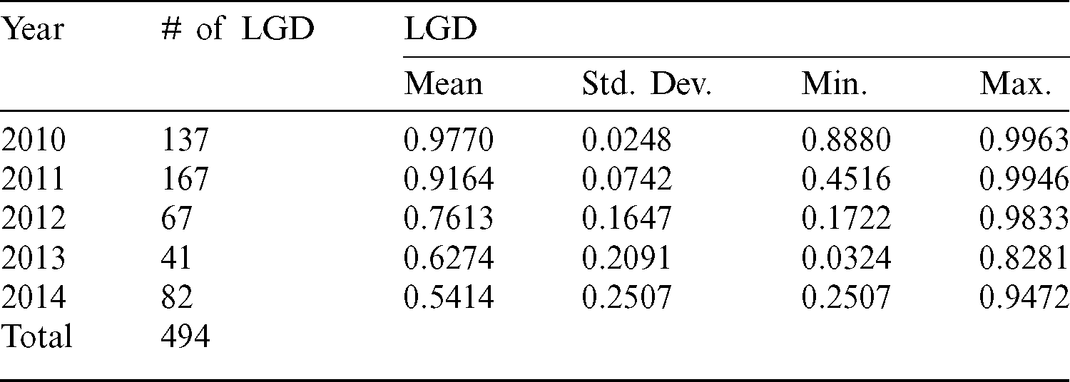
A sample data based on the credit portfolio of a banking institution in Jordan is used in our study. The credit bank portfolio was obtained from January 2010–December 2014. The portfolio capacity is 4393, and the overall number of defaults during the 5-year period is 494. The sample size is the same as the number of default, which is 494, and the LGD data lies between interval [0,1]. For the case study, a borrower is declared as default if he is unable to pay cash installment in a period of 3 months.
The number of defaults per annum and the summary statistics for the LGD data are presented in Tab. 2. The maximum number of LGD is recorded in years 2010 and 2011. It can be observed that the highest mean of LGD is 97.7% with 0.025 standard deviation in 2010. The high frequency of LGD in 2010 and 2011 in as results of Jordanian economy had late response to financial crisis, which occurred in 2008. The Amman stock exchange (ASE) after 2009 starts decreasing steadily until 2012 [41,42]. Indicated that performance of Jordanian Banks sector had negative effect after global financial crisis such as, share prices decreasing and non-performing assets increasing. Therefore, for this reason we see the number of default increased as result of financial crisis that effect of ability of borrowers to pay their borrowing money. However, the lowest mean of LGD is 54.1% with 0.251 standard deviation in year 2014. Furthermore, the minimum LGD is 3.2% in year 2013 and the maximum LGD is 99.6% in year 2010. The R-package is used for fitting the sample data to the parametric models [43].
Table 2: Summary statistics for LGD
Tab. 3 provides the results of the fitted parametric distributions. Beta distribution is the preferable model because it has the highest LogL and the lowest AIC and BIC. Further comparison can be obtained from the q–q plot, p–p plot, empirical and theoretical PDF, and empirical and theoretical CDF shown in Fig. 1. It can be found that beta distribution shows a better fit compared to other parametric distributions. Therefore the mean of Beta distribution can be used as the estimate of LGD for the credit portfolio [44].
The results from Tab. 3 show that beta distribution is the best model for fitting the sample data. Therefore, we consider beta regression with different link functions in order to explore the internal and external financial variables which significantly affect the LGD.
The descriptive statistics of the explanatory variables are shown in Tab. 4.
Table 4: Summary statistics for explanatory variables
Tab. 5 provides the parameter estimates and standard errors for Beta regressions, which are fitted using different link functions. All regression parameters are significant, at least at 0.10 level, except for beta regression with Cauchy link function where the estimate of LR is insignificant.
Table 5: Beta regression with different link functions
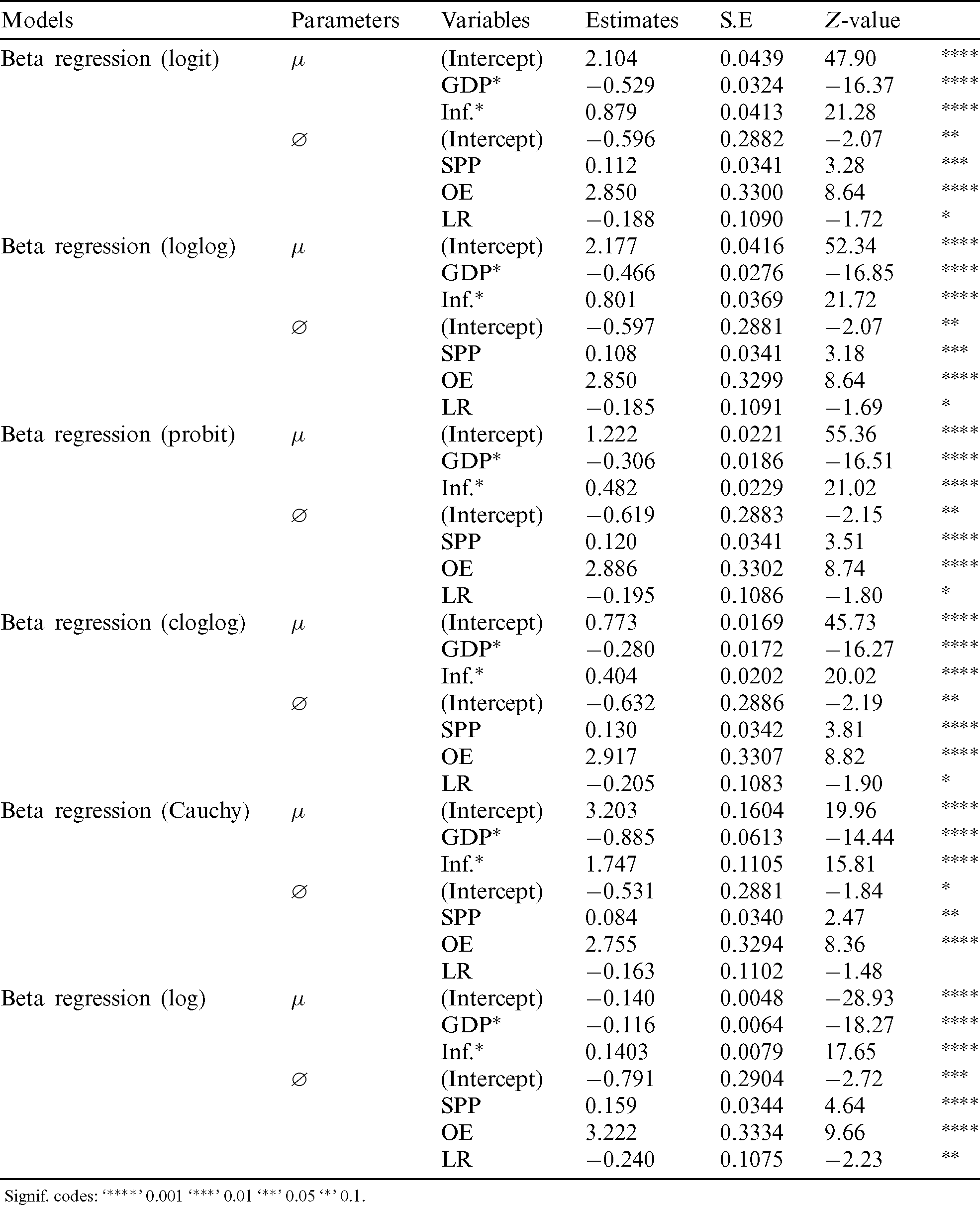
Signif. codes: ‘****’ 0.001 ‘***’ 0.01 ‘**’ 0.05 ‘*’ 0.1.
The estimates of GDP and Inf are highly significant for the mean  . GDP refer to a monetary measure of the market value of all final goods and services produced within the country’s border in a specific period of time (typically 1 year). An increasing GDP means that the economy is expanding, and firms are producing and selling more products or services. When GDP declines, the economy is depicted as being in a downturn. During downturn, fewer goods and services are being sold, business profits turn down, unemployment rises and government tax collections fall.
An increasing inflation rate (Inf) indicates a sustained increment in the prices of goods and services over a specific period of time. Inflation referred to a reduction in the purchasing power per unit of money. In other word, when inflation rate rises, each unit of currency buys fewer goods and services.
Our results show that a decreasing GDP growth rate resulted in an increasing LGD, while an increasing inflation rate resulted in an increasing LGD. The results are expected in an adverse economic conditions, where GDP diminishes and inflation rate increases as the default frequencies increase and the asset prices decrease [44], and consequently, the recovery rates decrease. When an economic prosperity resumes, the situation reverses, indicating that the capital requirements under these conditions would swing wildly. In general, a lower LGD is favored for calculating the expected loss (EL) of a banking institution. The results show that lower LGD is obtained when the GDP is higher and the inflation rate is lower.
Service pricing policy (SPP) ratio is measured as operating expenses divided by total liability. This ratio measures the funding for operating expenses by the total liability. Higher SPP is resulted when the relative decrease in total liability is more than the decrease in operating expenses. For our case, higher SPP decreases the variance of LGD. It is implied here that larger decreases in total liability resulted in less variations of LGD among the default borrowers.
Operating efficiency ratio (OE) is measured as total operating expenses divided by total operating revenues. The increase in OE is caused by the larger decrease in total operating revenue relative to the decrease in total operating expenses. Our case shows that higher OE decreases the LGD variance. It can be indicated here that larger reduction in total operating revenue leads to less variations of LGD among the default borrowers.
Cash ratio (cash and cash equivalents divided by current liability) is generally a more conservative liquidity ratio measure of a company’s ability to repay its short-term obligations, using only the most liquid of assets, such as cash on hand, cash equivalents (sometimes referred to as marketable securities) and demand deposits. This measure tells creditors the company’s ability to pay all current liabilities immediately without having to sell or liquidate other assets. Higher LR is resulted when current liability has larger decrease than the decrease in cash and cash equivalents. Our results show that higher liquidity ratio (LR) indicates higher variance of LGD. It is implied here that a larger decrease in current liability resulted in more variations of LGD among the default cases. In general, lower variance of LGD is favored in terms of risk measures. The results show that lower variance is obtained when we have higher SPP, higher OE, and lower LR.
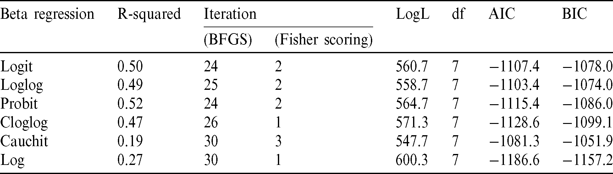
Further results can be seen in Tab. 6, where the R-squared, log likelihood, AIC and BIC for each model are provided. Since beta regression with probit link function has the highest R-squared, while having accepted measurements for logL, AIC and BIC, this model is chosen as the best regression model for explaining the relationship between LGD and financial variables.
Table 6: Beta regression with R-squared, AIC and BIC
In the context of credit portfolio, LGD is the percentage of exposure that will be lost if a default occurs. Uncertainty with respect to the actual LGD is an important source of risks of credit portfolio, in addition to default risk. In this study, several parametric distributions were used to estimate LGD based on a sample of credit portfolio collected from a bank in Jordan from the period of 2010–2014. The results show that Beta distribution is the best parametric model for estimating LGD based on the following tests; logL, AIC and BIC. Several financial variables were then incorporated to the sample data to find the macro- and micro-economics determinants of LGD. The results show that Beta regression with probit link function has the highest R-squared with accepted measurements for logL, AIC and BIC. The results from beta regression models show that macroeconomic variables (GDP and Inflation rate) are significant for the mean parameter  , while microeconomic variables (SPP, OE and LR) are significant for the precision parameter (
 ).In particular, a decreasing GDP growth rate resulted in an increasing LGD, while an increasing inflation rate resulted in an increasing LGD. In terms of LGD risks, the variance (risks) of LGD are lower with lower SPP and lower OP, but higher with lower LR. We have proposed successfully the significant microeconomic variables which affect on precision parameter (
 ) and compared between six different link functions (Logit, loglog, probit, cloglog, cauchit, and log) by Beta regression.
Funding Statement: This research is supported by the Fundamental Research Grant Scheme/ Ministry of Education Malaysia [Research No.: FRGS/1/2019/STG06/UKM/01/5] and the Research University Grant/Universiti Kebangsaan Malaysia [Research No.: GUP-2019-031]. Initials of authors who received the grant: N. Ismail.
Conflicts of Interest: The authors declare that they have no conflicts of interest to report regarding the present study.
1. J. J. Jaber, N. Ismail and S. N. M. Ramli. (2017). “Credit risk assessment using survival analysis for progressive right-censored data: A case study in Jordan,” Journal of Internet Banking and Commerce, vol. 22, no. 1, pp. 1–18.
2. B. Kollar and T. Kliestik. (2014). “Simulation approach in credit risk models,” in 4th Int. Conf. on Applied Social Science, Information Engineering Research Institute, Advances in Education Research, vol. 15, pp. 150–155.
3. E. I. Altman. (1989). “Measuring corporate bond mortality and performance,” Journal of Finance, vol. 44, no. 4, pp. 909–922.
4. V. V. Acharya, S. T. Bharath and A. Srinivasan. (2003). Understanding the Recovery Rates on Defaulted Securities. UK: Centre for Economic Policy Research.
5. P. Nickell, W. Perraudin and S. Varotto. (2000). “Stability of rating transitions,” Journal of Banking & Finance, vol. 24, no. 1–2, pp. 203–227.
6. J. Dermine and C. N. De Carvalho. (2006). “Bank loan losses-given-default: A case study,” Journal of Banking & Finance, vol. 30, no. 4, pp. 1219–1243.
7. H. Z. Chen. (2018). “A new model for bank loan loss-given-default by leveraging time to recovery,” Journal of Credit Risk, vol. 14, no. 3, pp. 1–29.
8. Y. Tanoue, A. Kawada and S. Yamashita. (2017). “Forecasting loss given default of bank loans with multi-stage model,” International Journal of Forecasting, vol. 33, no. 2, pp. 513–522.
9. L. Thompson and T. Brandenburger. (2019). “Survival analysis methods to predict loss rates in credit card portfolios,” in SDSU Data Science Sym. Session, South Dakota State University, USA, vol. 31.
10. M. Pykhtin. (2003). “Recovery rates: Unexpected recovery risk,” Risk-London-Risk Magazine Limited, vol. 16, no. 8, pp. 74–79.
11. T. Bellotti and J. Crook. (2008). Modelling and Estimating Loss Given Default for Credit Cards. University of Edinburgh Business School, UK, CRC Working Paper, pp. 1–15.
12. M. Bruche and C. González-Aguado. (2010). “Recovery rates, default probabilities, and the credit cycle,” Journal of Banking and Finance, vol. 34, no. 4, pp. 754–764.
13. X. Huang and C. W. Oosterlee. (2011). “Generalized beta regression models for random loss given default,” Journal of Credit Risk, vol. 7, no. 4, pp. 45–70.
14. T. Bellotti and J. Crook. (2012). “Loss given default models incorporating macroeconomic variables for credit cards,” International Journal of Forecasting, vol. 28, no. 1, pp. 171–182.
15. R. Calabrese. (2012). “Estimating bank loans loss given default by generalized additive models,” Technical Report University College Dublin Geary Institute, Working Paper, vol. 201224, pp. 1–17.
16. G. Loterman, I. Brown, D. Martens, C. Mues and B. Baesens. (2012). “Benchmarking regression algorithms for loss given default modeling,” International Journal of Forecasting, vol. 28, no. 1, pp. 161–170.
17. P. Li, M. Qi, X. Zhang and X. Zhao. (2016). “Further investigation of parametric loss given default modeling,” Journal of Credit Risk, Forthcoming, vol. 12, no. 4, pp. 17–47.
18. A. Hamerle, M. Knapp and N. Wildenauer. (2006). Modelling Loss Given Default: A “Point in Time” Approach, B. Engelmann and R. Rauhmeier, New York: Springer, pp.127–142.
19. S. Krüger and D. Rösch. (2017). “Downturn LGD modeling using quantile regression,” Journal of Banking & Finance, vol. 79, pp. 42–56.
20. BCBS. (2004). “Base II: International convergence of capital measurement and capital standards: A revised framework,” in Basel Committee on Banking Supervision. Basel: Bank for International Settlements.
21. BCBS. (2004). “Basel II: Background note on LGD quantification,” in Basel Committee on Banking Supervision. Basel: Bank for International Settlements.
22. BCBS. (2005). Basel II: Guidance on paragraph 468 of the framework document. Basel Committee on Banking Supervision. Basel: Bank for International Settlements.
23. E. I. Altman, B. Brady, A. Resti and A. Sironi. (2005). “The link between default and recovery rates: Theory, empirical evidence, and implications,” Journal of Business, vol. 78, no. 6, pp. 2203–2228.
24. S. Figlewski, H. Frydman and W. Liang. (2012). “Modeling the effect of macroeconomic factors on corporate default and credit rating transitions,” International Review of Economics and Finance, vol. 21, no. 1, pp. 87–105.
25. V. V. Acharya, S. T. Bharath and A. Srinivasan. (2007). “Does industry-wide distress affect defaulted firms? Evidence from creditor recoveries,” Journal of Financial Economics, vol. 85, no. 3, pp. 787–821.
26. S. Caselli, S. Gatti and F. Querci. (2008). “The sensitivity of the loss given default rate to systematic risk: New empirical evidence on bank loans,” Journal of Financial Services Research, vol. 34, no. 1, pp. 1–34.
27. P. Grippa, S. Iannotti and F. Leandri. (2005). “Recovery rates in the banking industry: Stylised facts emerging from Italian experience,” in Recovery Risk: The Next Challenge in Credit Risk Management. London: Riskbooks, pp. 121–141.
28. J. Frye. (2000). “Depressing recoveries,” Risk-London-Risk Magazine Limited, vol. 13, no. 11, pp. 108–111.
29. L. Andersen and J. Sidenius. (2004). “Extensions to the Gaussian copula: Random recovery and random factor loadings,” Journal of Credit Risk, vol. 1, no. 1, pp. 5.
30. K. Düllmann and M. Gehde-Trapp. (2004). “Systematic risk in recovery rates: An empirical analysis of US corporate credit exposures,” in Discussion Paper, Banking and Financial Supervision, Deutsche Bundesbank Frankfurt, Germany, pp. 1–44.
31. D. Rösch and H. Scheule. (2006). A Multi-Factor Approach for Systematic Default and Recovery Risk, in the Basel II Risk Parameters. Berlin: Springer, 105–125.
32. J. Zhang and L. C. Thomas. (2012). “Comparisons of linear regression and survival analysis using single and mixture distributions approaches in modelling LGD,” International Journal of Forecasting, vol. 28, no. 1, pp. 204–215.
33. M. Qi and X. Zhao. (2011). “Comparison of modeling methods for loss given default,” Journal of Banking & Finance, vol. 35, no. 11, pp. 2842–2855.
34. G. Schwarz. (1978). “Estimating the dimension of a model,” Annals of Statistics, vol. 6, no. 2, pp. 461–464.
35. H. Akaike. (1969). “Fitting autoregressive models for prediction,” Annals of the Institute of Statistical Mathematics, vol. 21, no. 1, pp. 243–247.
36. S. Ferrari and F. Cribari-Neto. (2004). “Beta regression for modelling rates and proportions,” Journal of Applied Statistics, vol. 31, no. 7, pp. 799–815.
37. P. McCullagh and J. Nelder. (1989). Generalized Linear Models. London: Chapman and Hall.
38. A. V. Rocha and A. B. Simas. (2011). “Influence diagnostics in a general class of beta regression models,” Test, vol. 20, no. 1, pp. 95–119.
39. A. C. Atkinson. (1985). Plots, Transformation and Regression: An Introduction to Graphical Methods of Diagnostic Regression Analysis. Oxford: Clarendon Press.
40. A. B. Simas, W. Barreto-Souza and A. V. Rocha. (2010). “Improved estimators for a general class of beta regression models,” Computational Statistics and Data Analysis, vol. 54, no. 2, pp. 348–366.
41. A. A. A. Sharabati and A. N. I. Nour. (2014). “Impact of global financial crisis on Amman Stock Exchange (ASE) market,” Journal of Baghdad College of Economic sciences University, vol. 2014, no. 4, pp. 540–558.
42. B. A. Dalaien. (2016). “Impact of global financial crisis on banking sector of India and Jordan,” Academic Journal of Economic Studies, vol. 2, no. 1, pp. 79–95.
43. N. Belgorodski, M. Greiner, K. Tolksdorf, K. Schueller, M. Flor. (2017). et al., “Rriskdistributions: fitting distributions to given data or known quantiles,” The Comprehensive R Archive Network, pp. 1–68.
44. G. Van Vuuren, R. De Jongh and T. Verster. (2017). “The impact of PD-LGD correlation on expected loss and economic capital,” International Business and Economics Research Journal, vol. 16, no. 3, pp. 157–170.
 | This work is licensed under a Creative Commons Attribution 4.0 International License, which permits unrestricted use, distribution, and reproduction in any medium, provided the original work is properly cited. |