DOI:10.32604/cmc.2021.014675
| Computers, Materials & Continua DOI:10.32604/cmc.2021.014675 | |
| Article |
An Adjustable Variant of Round Robin Algorithm Based on Clustering Technique
1Faculty of Computers and Information, South Valley University, Qena, 83523, Egypt
2Research Institute for Information Technology, Kyushu University, Fukuoka, 819-0395, Japan
*Corresponding Author: Samih M. Mostafa. Email: samih_montser@sci.svu.edu.eg
Received: 08 October 2020; Accepted: 25 October 2020
Abstract: CPU scheduling is the basic task within any time-shared operating system. One of the main goals of the researchers interested in CPU scheduling is minimizing time cost. Comparing between CPU scheduling algorithms is subject to some scheduling criteria (e.g., turnaround time, waiting time and number of context switches (NCS)). Scheduling policy is divided into preemptive and non-preemptive. Round Robin (RR) algorithm is the most common preemptive scheduling algorithm used in the time-shared operating systems. In this paper, the authors proposed a modified version of the RR algorithm, called dynamic time slice (DTS), to combine the advantageous of the low scheduling overhead of the RR and favor short process for the sake of minimizing time cost. Each process has a weight proportional to the weights of all processes. The process’s weight determines its time slice within the current period. The authors benefit from the clustering technique in grouping the processes that are similar in their attributes (e.g., CPU service time, weight, allowed time slice (ATS), proportional burst time (PBT) and NCS). Each process in a cluster is assigned the average of the processes’ time slices in this cluster. A comparative study of six popular scheduling algorithms and the proposed approach on nine groups of processes vary in their attributes was performed and the evaluation was measured in terms of waiting and turnaround times, and NCS. The experiments showed that the proposed algorithm gives better results.
Keywords: Clustering; CPU scheduling; round robin; turnaround time; waiting time
This section is divided into two subsections: (i) CPU scheduling, and (ii) Clustering technique.
Allocating and de-allocating the CPU to a specific process is known as process scheduling (also known as CPU scheduling) [1–3]; the piece of the operating system that performs these functions is called the scheduler. From the processes that are waiting in the memory to receive service from the CPU, the scheduler chooses the next process to be assigned to the CPU. The scheduling scheme may be non-preemptive or preemptive, and many CPU scheduling algorithms have been suggested. First Come First Served (FCFS) algorithm executes processes upon their order of arrives. Shortest Job First (SJF) algorithm selects the process with the shortest burst time. Under Shortest Remaining Time First (SRTF) algorithm, the execution of the running process is paused when a process with shorter burst time arrives. Under priority scheduling, the execution of the running process is paused when a process with higher priority arrives [4].
The most common of the preemptive scheduling algorithms is the RR scheduling [5], known hereafter as Standard RR (SRR), used in timesharing and real-time operating systems [6]. In RR scheduling, the operating system is driven by a regular interrupt by the system timer after a short fixed interval called standard time slice (STS) [7–10]. After that interruption, the scheduler switches the context to the next process selected from the circular queue [11,12]. Thus, all processes are given a chance to receive CPU service time for a short fixed period. The fixed time slice influences the efficiency of RR algorithm; short time slice leads to high overheads, and long time slice may leads to starvation between processes. In addition, scheduling criteria (i.e., waiting time, turnaround time, and NCS) affect performance of the scheduling algorithm [13–15].
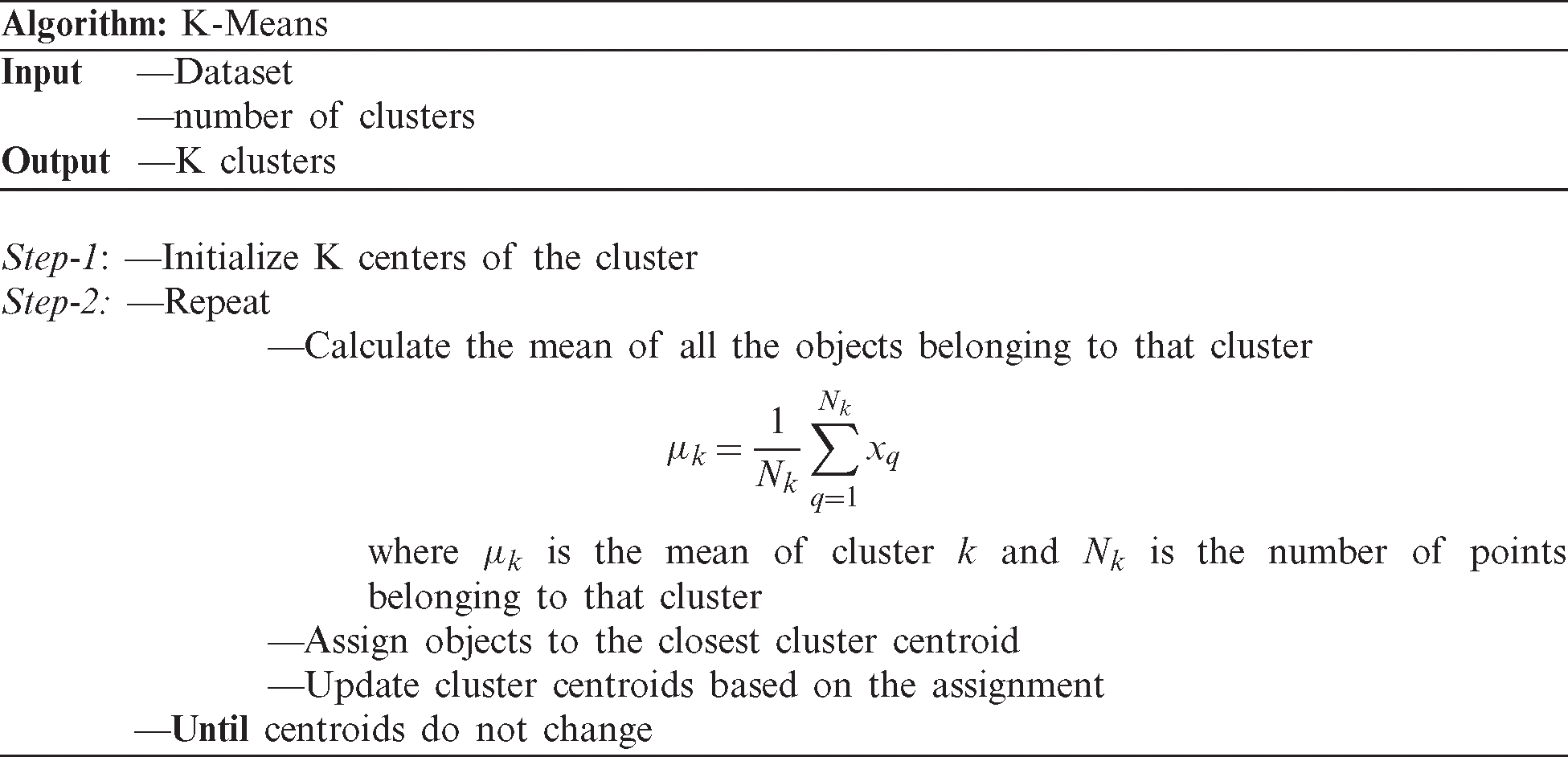
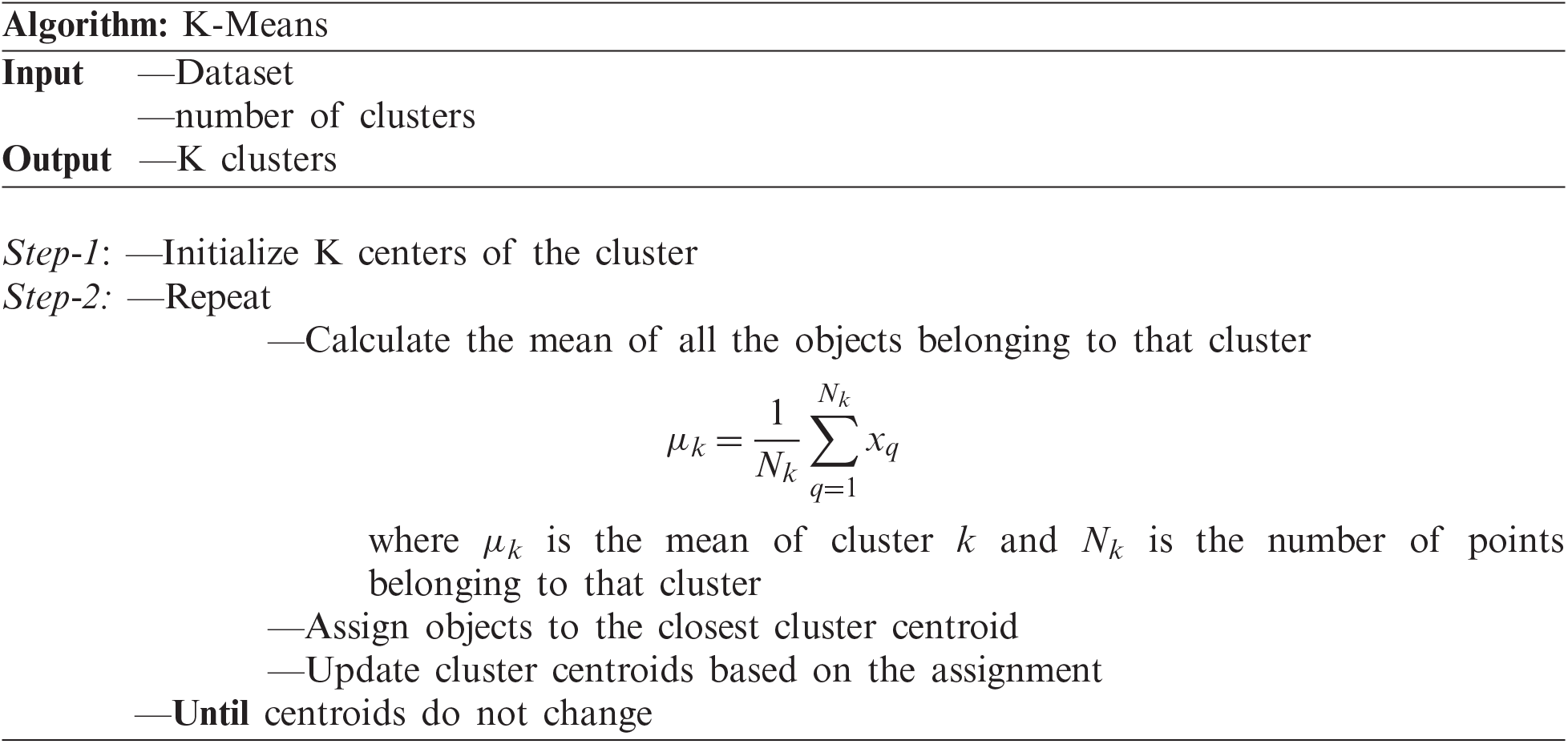
Clustering means dividing the data into groups that are useful and meaningful [16]; greater homogeneity (or similarity) within a cluster and greater difference between clusters bring about better clustering. Clustering is a type of classification in that it generates labels of the clusters [17,18]. Classification of data can be completed using clustering without prior knowledge. A clustering algorithm is the process of dividing abstract or physical object into a collection of similar objects. Cluster is a collection of data points; points in the same cluster are like each other and different from points in other clusters. The type of the data determines the algorithm used in the clustering, for example, statistical algorithms are used for clustering numeric data, categorical data is clustered using conceptual algorithms, fuzzy clustering algorithms allow data point to be classified into all clusters with a degree of membership ranging from 0 to 1, this degree indicates the likeness of the data point to the mean of the cluster. Clustering algorithms are categorized into traditional and modern [19]. K-means is the most commonly and simplest clustering algorithm. Its simplicity comes from the use of the squared error as stopping criterion. In addition, the time complexity of the K-means algorithm is low O(nkt), where n: the number of objects, k: The number of clusters, and t: The number of iterations. K-means algorithm divides the dataset into K clusters ( ), represented by their centers or means to minimize some objective function that depends on the vicinity of the subjects to the cluster centroids. The function to be minimized in K-means is described in Eq. (1) [20].

where K is the number of the clusters set by the user,  is the weight of x,
 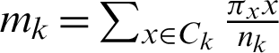 is the centroid of cluster Ck, and the function ‘dist’ computes the distance between the object x and the centroid
  ,
,  . The K-means clustering method requires all data to be numerical. The pseudo-code of K-means algorithm is as follows:
:
Determining the optimal number of clusters in a dataset is an issue in clustering. The most commonly clustering evaluation technique used is the Silhouette method which measures clustering quality by determining how well each data point lies within its cluster. The Silhouette method can be summarized as follows:
1. Apply the clustering algorithm for different values of k. For instance, by varying k from 1 to n clusters.
2. For each k, the total Within-cluster Sum of Square (WSS) is calculated.
3. Plot the curve of WSS according to the value of k.
4. The location of a knee in the curve indicates the appropriate number of clusters.
Eq. (2) defines the Silhouette coefficient (Si) of the ith data point.

where bi is the average distance between the ith data point and all data points in different clusters; ai, is the average distance between the ith data point and all other data points in the same cluster [16,21].
Motivation: The time slice used in RR scheduling algorithm influences the performance of the timesharing systems. The time slice used should be chosen to avoid starvation (resulted from choosing long time slice) and overheads of more context switches (resulted from choosing short time slice).
Organization: The rest of this paper is divided as follows: Section 2 discusses the related work. The proposed algorithm is presented in Section 3. Section 4 discusses the experimental implementation. Section 5 concludes this research work (see Fig. 1).
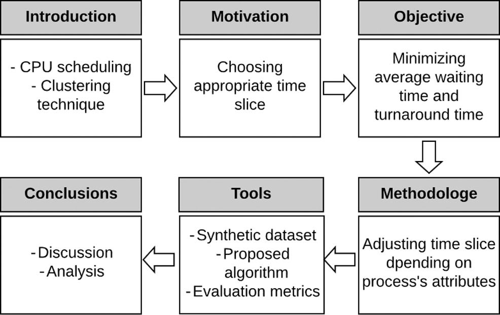
Figure 1: Organization of the paper
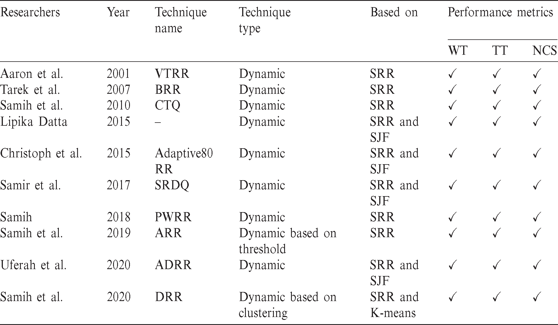
For better CPU performance in most of the operating systems, the RR scheduling algorithm is widely implemented. Many versions of the RR algorithm have been proposed to minimize turnaround and average waiting times. This section discusses the most common variants of the RR. Tab. 1 shows a comparison between the known variants of SRR. Variable Time Round-Robin scheduling (VTRR) is a dynamic version of the SRR algorithm proposed by Aaron et al. [22]. VTRR assigned a time slice to a process taking into consideration the time needed to all processes. A weighting version of SRR is proposed by Tarek et al. [23]. The authors groups the processes into five categories based on the burst times. The weight of a process is inversely proportional to its burst time; process with low weight receives less time and vice versa. If the burst time of a process less than or equal to 10 tu, it receives 100% of the time defined by SRR. If the burst time of a process less than or equal to 25 tu, it receives 80% of the time defined by SRR, and so on. Changeable Time Quantum (CTQ) is a dynamic version of SRR proposed by Samih et al. [14]. In every round, CTQ finds the time quantum that gives the smallest average waiting time, and the processes executes for this time. Modifying the time slice at the beginning of each round is another dynamic version of SRR proposed by Lipika [24], in which the time slice is calculated with respect to the residual burst times  in the successive rounds. Lipika benefited from SJF in which the processes are ordered increasingly based on their burst times (i.e., the process with the highest burst time will be at the tail of the ready queue and the process with the lowest burst time will be at the head of the queue) [25–27]. Adaptive80 RR is a dynamic variant of SRR proposed by Christoph and Jeonghw [6]. The time quantum equals process’s burst time at 80th percentile. The authors imitated Lipika’s [24] in sorting the processes in increasing order, and the time slice in each is calculated depending on the burst times of the processes in the queue. A hybrid scheduling technique based on SJF and SRR named SJF and RR with dynamic quantum (SRDQ) is proposed by Samir et al. [28]. SRDQ divided the queue into Q1 and Q2 based on the median; Q2 for long the processes (longer than the median) and Q1 for the short processes (shorter than the median). Like Lipika’s [24] and Adaptive80 RR [6] algorithms, SRDQ sorts the processes in the queue in ascending order in each subqueue. Proportional Weighted Round Robin (PWRR) is a modified version of SRR proposed by Samih [15]. PWRR assigns the time slice to a process proportional to its weigh which is calculated by dividing its burst time by the summation of all processes’ burst times in the queue. Adjustable Round Robin (ARR) is another dynamic version of the SRR proposed by Samih et al. [13]. Under a predefined condition, ARR gives short process a chance of execution until termination without interruption. Amended Dynamic Round Robin (ADRR) is a dynamic version of SRR proposed by Uferah et al. [12]. In every cycle, the time slice is adjusted based on the burst time of the process. Like Lipika’s [24], SRDQ [28] and Adaptive80 RR [6] algorithms, the processes are sorted in ascending order. Dynamic Round Robin (DRR) CPU scheduling algorithm is a dynamic version of the SRR algorithm based on clustering technique proposed by Samih et al. [29]. DRR starts by grouping similar processes in a cluster; the number of clusters is obtained from Silhouette method. Each cluster has a weight and is assigned a time slice, and all processes in a cluster are assigned the same time slice. They benefit from the clustering technique in grouping processes that resemble each other in their features.
Table 1: Comparison of common versions of SRR (WT denotes waiting time, and TT denotes turnaround time)
The processes’ weights (PW), ATS, PBT, and NCS depend on the process’s burst times (BT), and are calculated in the next subsections. The proposed work starts by grouping similar processes in clusters. The similarity between processes depends on BT, ATS, NCS, PW and PBT. K-means is the most commonly algorithm used in clustering. The proposed work consists of three phases: Data preparation, data clustering, and dynamic implementation.
In the data preparation phase, PW and NCS are calculated. The weight of the ith process (PWi) is calculated from Eq. (3):

where N is the number of the processes, and BTi is the burst time of the ith process. NCS is calculated from Eq. (4):
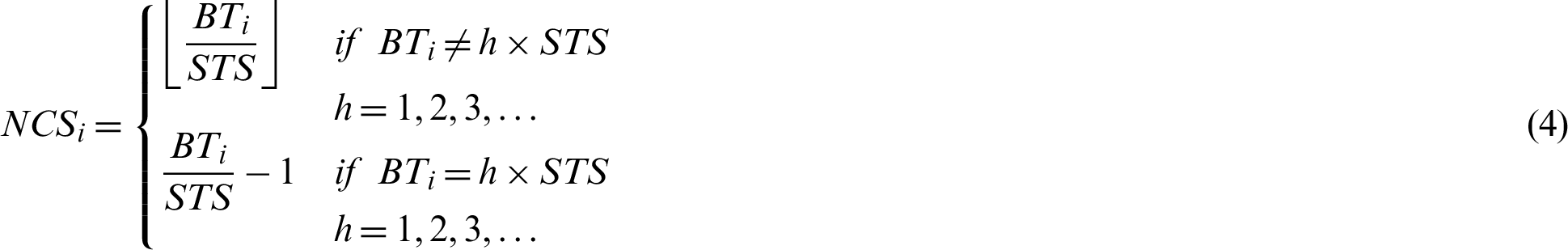
STS is determined by SRR, and  indicates the largest integer smaller than or equal to X. If the burst time of a process is greater than the STS, the time slice of this process equals STS. The ATS assigned to a process in a round is calculated from Eq. (5).

PBT of a process in a round is calculated from Eq. (6).

The proportional time slice (PTS) of a process in a round is calculated from Eq. (7).

In the data clustering phase, Silhouette method is used to find the optimum number, k, of clusters, then K-means algorithm clusters the data into k number. BT, PW, ATS, PBT and NCS are the clustering metrics used in the proposed work. Each data point is assigned to the nearest centroid, each group of points assigned to the same centroid results cluster. The assignment and updating steps are repeated until all centroids do not change. The Euclidean (L2) distance is used to quantify the notion of ‘closest’.
In the dynamic implementation, the process with long burst time results small PTS, which causes many NCS. To avoid overhead resulted from more NCS, a threshold which is an implementation choice is determined. The weight of the  cluster, CWl, is calculated from Eq. (8):

where Cavgl is the average of burst times in the lth cluster. Eq. (9) calculates the time slice assigned to the lth cluster (CTSl).

Each process  executes for CTSl. Awarding more time to the process that is close to its completion enables it to complete its execution and leave the queue, which in turn decreases the number of processes in the queue.
Unlike Previous works (e.g., Samih et al. [29]) which give short process in the current round an opportunity to run until termination under predefined condition, the proposed algorithm takes into account not only the current round, but also successive rounds. Depending on the process’s BT, the proposed algorithm gives it more time in the current and successive rounds according to Eq. (10):
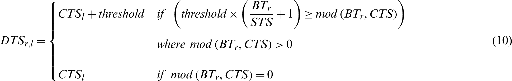
where  is the dynamic time slice assigned to process Pr in cluster l. In successive rounds, RBT will be updated according to Eq. (11). The proposed algorithm is described in Fig. 2.

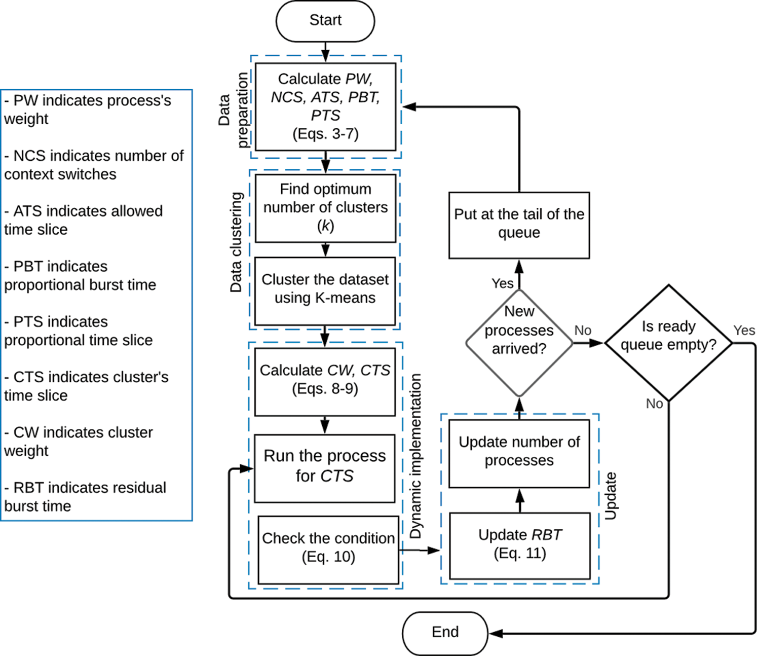
Figure 2: Algorithm flowchart
The following example illustrates the proposed technique. Tab. 2 contains the first dataset used in the experiments. The optimal number of clusters is indicated from the location of a knee in the curve in Fig. 3.
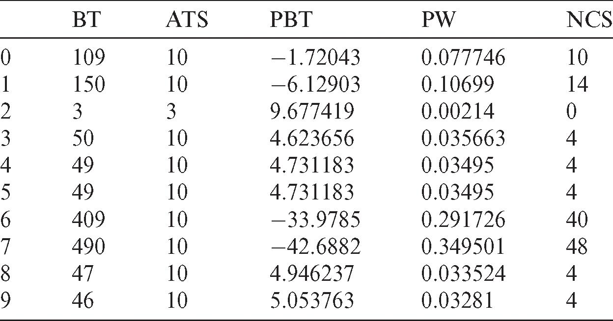
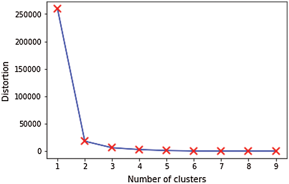
Figure 3: Optimal number of clusters ( )
)
Cluster 1 contains the 7th and 8th processes. Cluster 0 contains the others (Tab. 3).
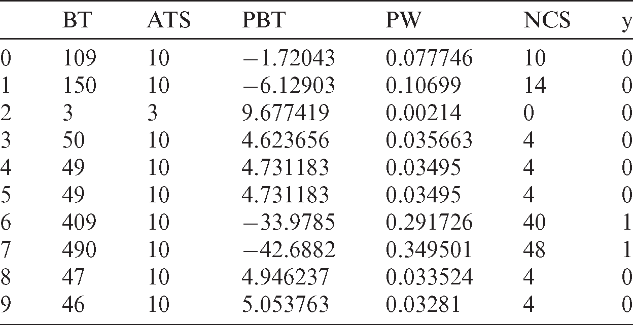
From Eq. (8), CW0 equals 0.981702176 tu, and CW1 equals 1.754574456 tu. From Eq. (9), CTS0 equals 6.41227 tu, and CTS1 equals 3.58773 tu. The 7th and 8th processes will be assigned 3.58773 tu, the others will be assigned 6.41227 tu.
The specifications of the computer used in the experiments are: Intel core i5-2400 (3.10 GHz) processor, 1 TB HDD, 16 GB memory, Python 3.7.6, and Gnu/Linux Fedora 28 OS.
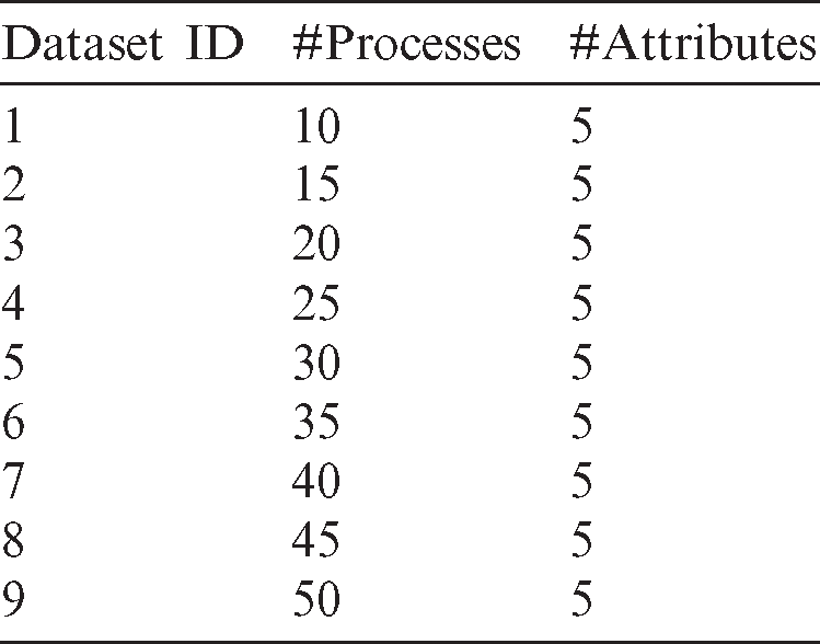
The performance of the compared algorithms was tested using nine synthetic datasets [29]. The burst times in each dataset are randomly generated. The number of process, BTs, NCSs, PBT, and ATSs in each dataset differ from the other. Detailed information on datasets is presented in Tab. 4.
Table 4: Datasets specifications. The first column presents the dataset ID, the second column presents the number of processes, and the third column presents the number of attributes (i.e., ATS, BT, PBT, PW, and NCS)
Six common algorithms; VTRR, SRR, ADRR PWRR, BRR and DRR were compared with the proposed algorithm on different nine collections of number of processes with different attributes. The experiments were performed in two cases; when the processes arrive at the same time, and when the processes arrive in different times.
– In the first case, the time consumed in the clustering is trivial and can be ignored. Fig. 4 shows the average waiting times and turnaround times comparison. Fig. 5 shows the NCS comparison. Fig. 6 shows the improvement percentage of the proposed algorithm over the compared algorithms. Tab. A1 shows a comparison of the time cost between the compared algorithms in terms of average waiting and turnaround times and NCS. Tab. A2 shows the improvement percentages of the proposed algorithm over the six scheduling algorithms.
– In the second case, new processes arrive to the queue; therefore, the clustering is repeated in every round. Fig. 7 shows the average waiting times and turnaround times comparison. Fig. 8 shows the NCS comparison. Fig. 9 shows the improvement percentage of the proposed algorithm over the six scheduling algorithms. Tab. B1 shows the running times comparison between the compared algorithms. Tab. B2 shows the average waiting time and turnaround time comparison between the compared algorithms. Tab. B3 shows the improvement percentages of the proposed algorithm over the six scheduling algorithms in terms of average waiting and turnaround times, and NCS.
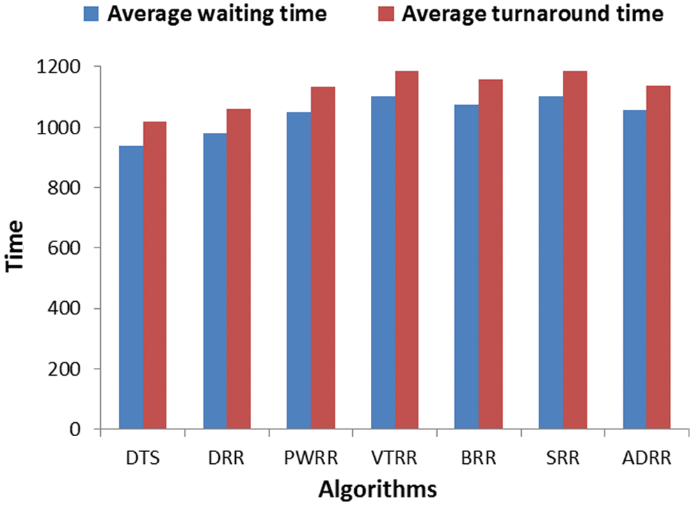
Figure 4: Comparing algorithms’ time cost (case 1)
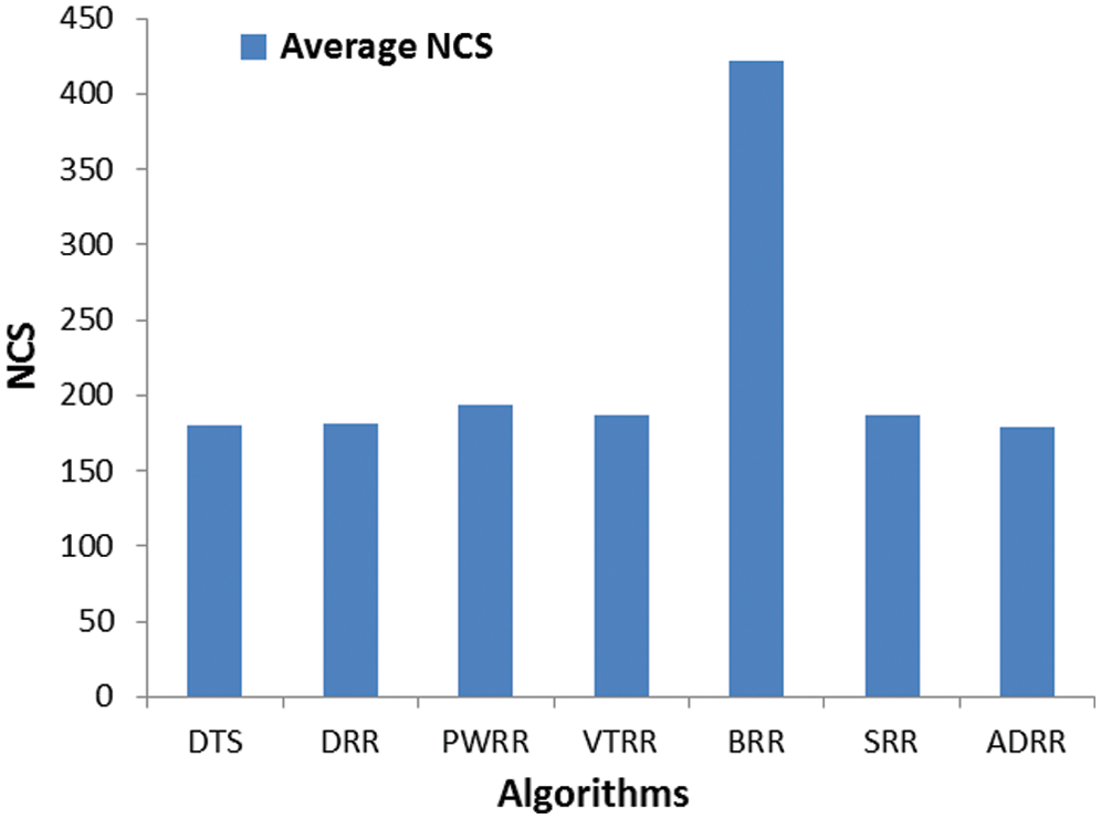
Figure 5: Comparing algorithms’ NCS (case 1)
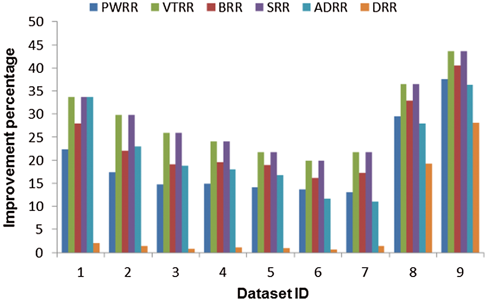
Figure 6: Improvement percentage of the proposed algorithm over the compared algorithms (case 1)
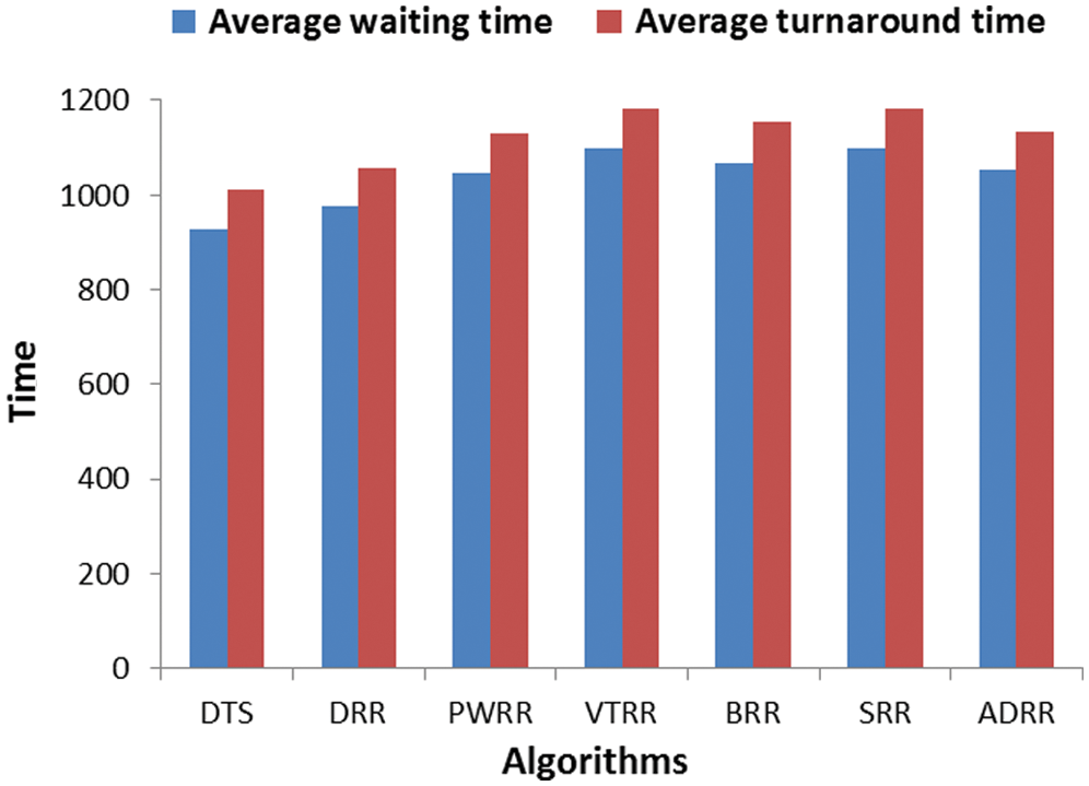
Figure 7: Comparing algorithms’ time cost (case 2)
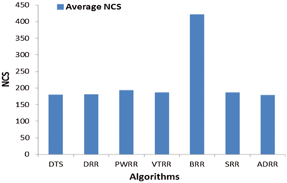
Figure 8: Comparing algorithms’ NCS (case 2)
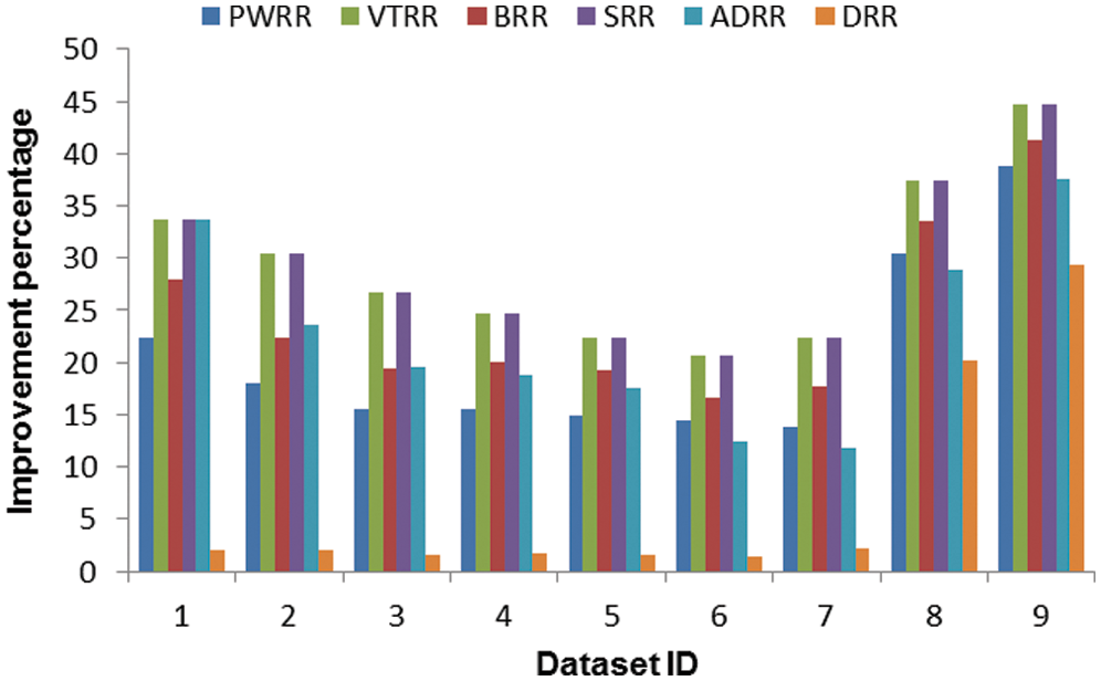
Figure 9: Improvement percentage of the proposed algorithm over the compared algorithms (case 2)
This paper introduced a dynamic version of SRR. The proposed algorithm reduces the scheduling time cost (i.e., waiting time and turnaround time). Unlike SRR which uses a fixed slice of time, the proposed algorithm assigns a time slice to a group of similar processes and each process in this group runs for this time. The similarity between the processes in a group is determined using the clustering technique depending on the attributes of these processes. The most important attribute is the burst time that determines other attributes (i.e., number of allocations to CPU, weights, and the allowed time slice in a round). Clustering technique uses these attributes to cluster the processes. Every process in a cluster is assigned a time slice equal to the average of all allowed time slices in the group. In a round, some processes may complete their execution times and leave the queue; therefore, in the successive rounds, the number and burst times of survived processes will be updated. If all processes arrived at the same time, the clustering is applied once. On the other hand, if the processes arrive sequentially, clustering is applied in each round. The proposed algorithm endows the process that is close to complete with more time in the current round. In addition, the proposed algorithm gives a process more time in the current and successive rounds according to the condition in Eq. (10). The comparison was done between the proposed algorithm and six common algorithms from the point of view of waiting time, turnaround time, and NCS. The results showed that the proposed algorithm outperformed the compared algorithms.
Funding Statement: The author(s) received no specific funding for this study.
Conflicts of Interest: The authors declare that they have no conflicts of interest to report regarding the present study.
1 K. Chandiramani, R. Verma and M. Sivagami. (2019). “A modified priority preemptive algorithm for CPU scheduling,” Procedia Computer Science, vol. 165, pp. 363–369. [Google Scholar]
2 I. S. Rajput and D. Gupta. (2012). “A priority based round robin CPU scheduling algorithm for real time systems,” Journal of Advanced Engineering Technologies, vol. 1, no. 3, pp. 1–11.
3 M. R. Reddy, V. V. D. S. S. Ganesh, S. Lakshmi and Y. Sireesha. (2019). “Comparative analysis of CPU scheduling algorithms and their optimal solutions,” in 2019 3rd Int. Conf. on Computing Methodologies and Communication (ICCMCErode, India, pp. 255–260. [Google Scholar]
4 A. Silberschatz, P. B. Galvin and G. Gagne. (2018). Operating System Concepts-10th. John Wiley & Sons, Inc. [Google Scholar]
5 J. Sunil, V. G. Anisha Gnana and V. T. Karthija. (2018). Fundamentals of Operating Systems Concepts. Germany, Saarbrucken: Lambert Academic Publications. [Google Scholar]
6 C. McGuire and J. Lee. (2015). “The adaptive80 round robin scheduling algorithm,” in Transactions on Engineering Technologies. Dordrecht, The Netherlands: Springer, pp. 243–258. [Google Scholar]
7 T. Wilmshurst. (2010). Designing Embedded Systems with Pic Microcontrollers, 2 ed., Oxford: Elsevier. [Google Scholar]
8 P. Singh, A. Pandey and A. Mekonnen. (2015). “Varying response ratio priority: A preemptive CPU scheduling algorithm (VRRP),” Journal of Computer and Communications, vol. 3, no. 4, pp. 40–51.
9 M. U. Farooq, A. Shakoor and A. B. Siddique. (2017). “An efficient dynamic round robin algorithm for CPU scheduling,” in 2017 Int. Conf. on Communication, Computing and Digital Systems (C-CODEIslamabad, Pakistan, pp. 244–248.
10 A. A. Alsulami, Q. A. Al-Haija, M. I. Thanoon and Q. Mao. (2019). “Performance evaluation of dynamic round robin algorithms for CPU scheduling,” in 2019 Southeast Conf., Huntsville, AL, USA, pp. 1–5. [Google Scholar]
11 A. Singh, P. Goyal and S. Batra. (2010). “An optimized round robin scheduling algorithm for CPU scheduling,” International Journal on Computer Science and Engineering, vol. 2, no. 7, pp. 2383–2385. [Google Scholar]
12 U. Shafi, M. Shah, A. Wahid, K. Abbasi, Q. Javaid. (2020). et al., “A novel amended dynamic round robin scheduling algorithm for timeshared systems,” International Arab Journal of Information Technology, vol. 17, no. 1, pp. 90–98. [Google Scholar]
13 S. M. Mostafa and H. Amano. (2019). “An adjustable round robin scheduling algorithm in interactive systems,” Information Engineering Express (IEE), vol. 5, no. 1, pp. 11–18. [Google Scholar]
14 S. M. Mostafa, S. Z. Rida and S. H. Hamad. (2010). “Finding time quantum of round robin CPU scheduling algorithm in general computing systems using integer programming,” International Journal of New Computer Architectures and their Applications, vol. 5, pp. 64–71. [Google Scholar]
15 S. M. Mostafa. (2018). “Proportional weighted round robin: A proportional share CPU scheduler in time sharing systems,” International Journal of New Computer Architectures and their Applications, vol. 8, no. 3, pp. 142–147. [Google Scholar]
16 U. G. Inyang, O. O. Obot, M. E. Ekpenyong and A. M. Bolanle. (2017). “Unsupervised learning framework for customer requisition and behavioral pattern classification,” Modern Applied Science, vol. 11, no. 9, pp. 151–164. [Google Scholar]
17 A. Lengyel and Z. Botta-Dukát. (2019). “Silhouette width using generalized mean–-A flexible method for assessing clustering efficiency,” Ecology and Evolution, vol. 9, no. 23, pp. 13231–13243. [Google Scholar]
18 A. Starczewski and A. Krzyżak. (2015). “Performance evaluation of the silhouette index bt: Artificial intelligence and soft computing,” in Artificial Intelligence and Soft Computing, Lecture Notes in Computer Science, vol. 9120. Cham: Springer, pp. 49–58. [Google Scholar]
19 D. Xu and Y. Tian. (2015). “A comprehensive survey of clustering algorithms,” Annals of Data Science, vol. 2, no. 2, pp. 165–193. [Google Scholar]
20 J. Wu. (2012). Cluster Analysis and K-means Clustering: An Introduction, Advances in K-means Clustering. Berlin Heidelberg: Springer, pp. 1–16. [Google Scholar]
21 Y. Liu, Z. Li, H. Xiong, X. Gao and J. Wu. (2010). “Understanding of Internal Clustering Validation Measures,” in 2010 IEEE Int. Conf. on Data Mining, ICDM, Sydney, NSW, Australia, pp. 911–916. [Google Scholar]
22 A. Harwood and H. Shen. (2001). “Using fundamental electrical theory for varying time quantum uniprocessor scheduling,” Journal of Systems Architecture, vol. 47, no. 2, pp. 181–192. [Google Scholar]
23 T. Helmy. (2007). “Burst round robin as a proportional-share scheduling algorithm,” in Proc. of the 4th IEEE-GCC Conf. on Towards Techno-Industrial Innovations, Bahrain, pp. 424–428. [Google Scholar]
24 L. Datta. (2015). “Efficient round robin scheduling algorithm with dynamic time slice,” International Journal of Education and Management Engineering, vol. 5, no. 2, pp. 10–19. [Google Scholar]
25 S. Zouaoui, L. Boussaid and A. Mtibaa. (2019). “Improved time quantum length estimation for round robin scheduling algorithm using neural network,” Indonesian Journal of Electrical Engineering and Informatics, vol. 7, no. 2, pp. 190–202. [Google Scholar]
26 A. Pandey, P. Singh, N. H. Gebreegziabher and A. Kemal. (2016). “Chronically evaluated highest instantaneous priority next: A novel algorithm for processor scheduling,” Journal of Computer and Communications, vol. 4, no. 4, pp. 146–159.
27 N. Srinivasu, A. S. V. Balakrishna and R. D. Lakshmi. (2015). “An augmented dynamic round robin CPU,” Journal of Theoretical and Applied Information Technology, vol. 76, no. 1, pp. 118–126. [Google Scholar]
28 S. Elmougy, S. Sarhan and M. Joundy. (2017). “A novel hybrid of shortest job first and round Robin with dynamic variable quantum time task scheduling technique,” Journal of Cloud Computing, vol. 6, no. 1, pp. 1–12. [Google Scholar]
29 S. M. Mostafa and H. Amano. (2020). “Dynamic round robin CPU scheduling algorithm based on K-means clustering technique,” Applied Sciences, vol. 10, no. 15, pp. 1–4. [Google Scholar]
Appendix A
Table A1: Average waiting time and turnaround time comparison between the proposed algorithm and six scheduling algorithms (case 1)
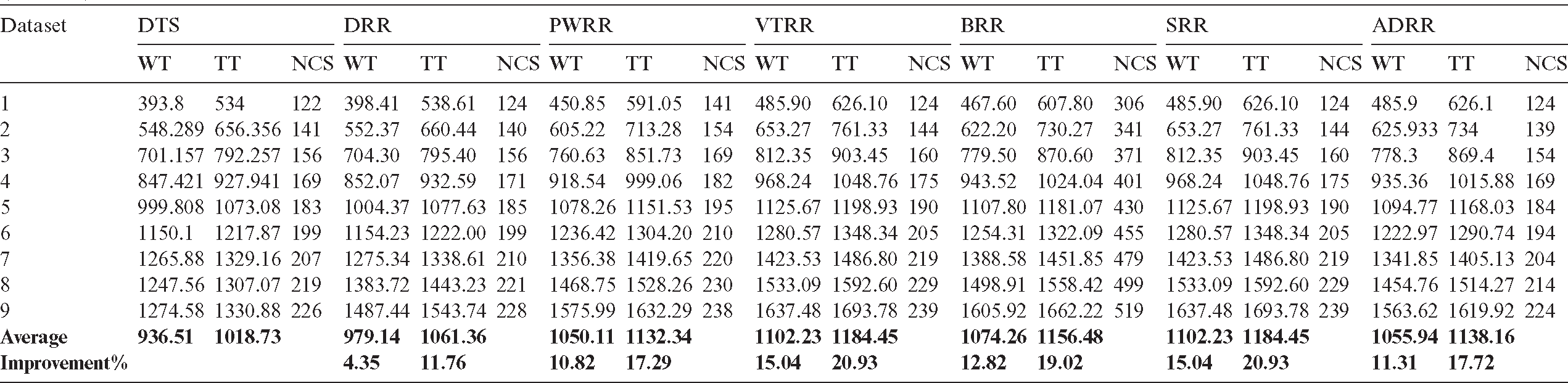
Table A2: Improvement percentages of the proposed algorithm over six scheduling algorithms (case 1)
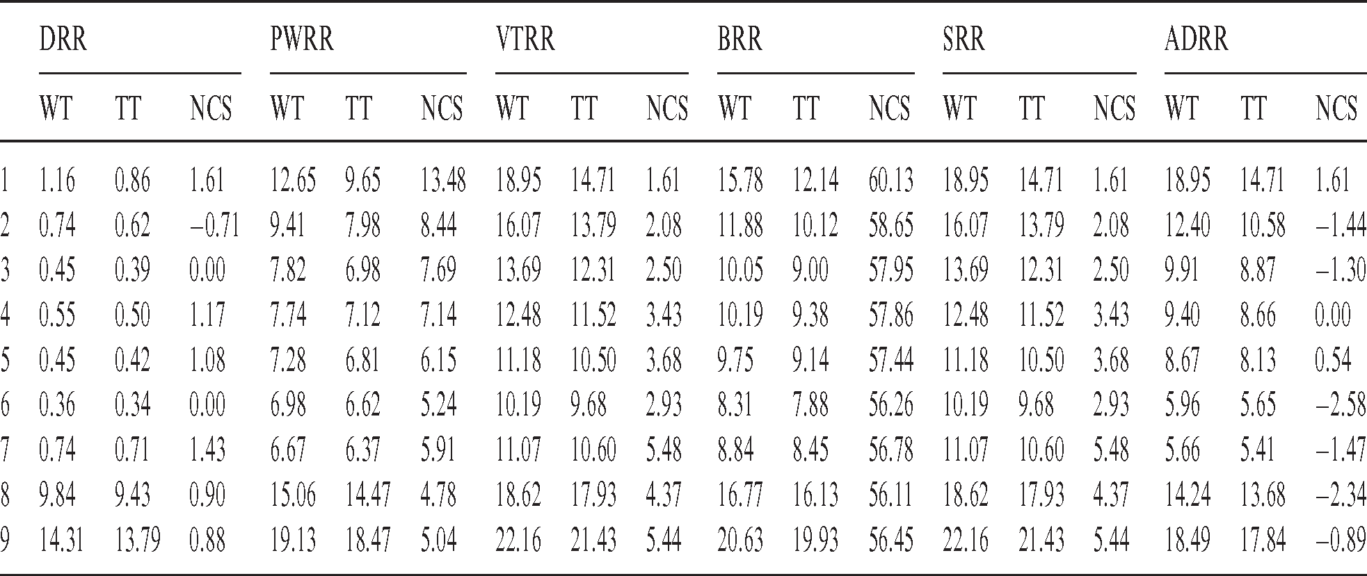
Table B1: Running times comparison between the proposed algorithm and six scheduling algorithms (case 2)
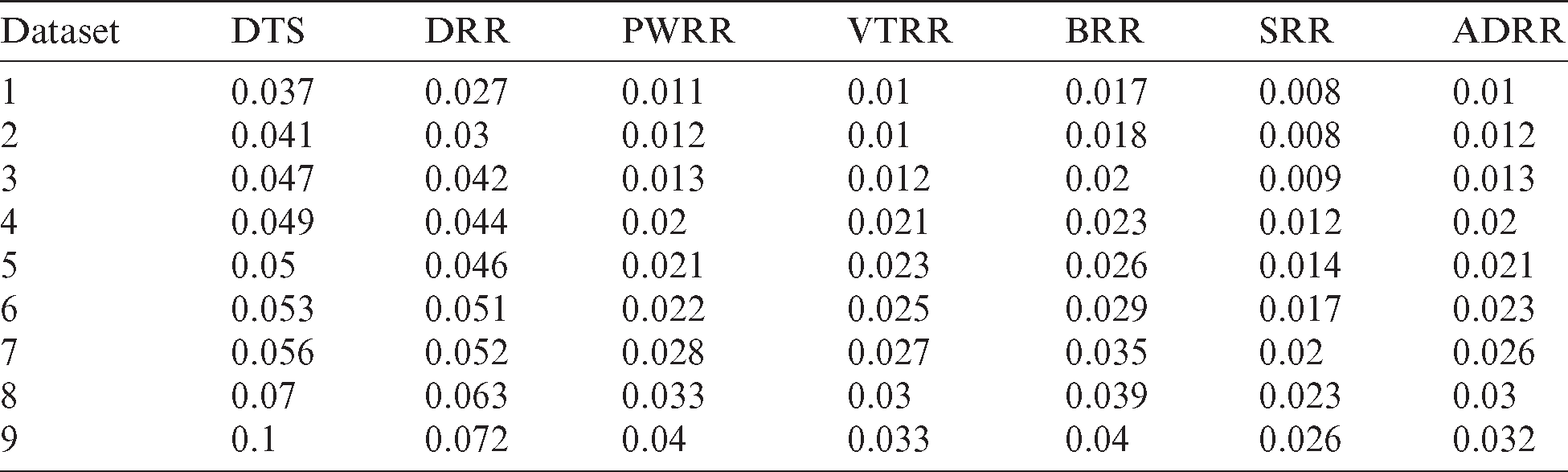
Table B2: Average waiting time and turnaround time comparison between the proposed algorithm and six scheduling algorithms (case 2)
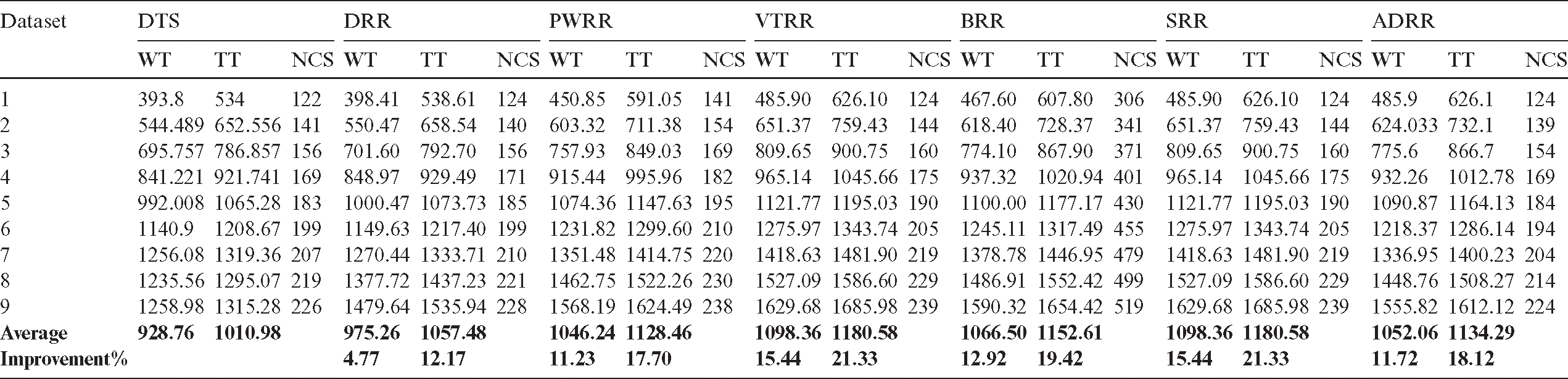
Table B3: Improvement percentages of the proposed algorithm over six scheduling algorithms (case 2)