DOI:10.32604/cmc.2021.012200
| Computers, Materials & Continua DOI:10.32604/cmc.2021.012200 | |
| Article |
Dynamical Behaviors of Nonlinear Coronavirus (COVID-19) Model with Numerical Studies
1Department of Mathematics, College of Science, Taif University, Taif, 21944, Saudi Arabia
2Department of Mathematics, Zagazig University, Zagazig, 44519, Egypt
3Department of Mathematics, Al-Azher University, Nasr City, 11884, Egypt
*Corresponding Author: Amr M. S. Mahdy. Emails: k.gepreel@tu.edu.sa; amattaya@tu.edu.sa
Received: 19 June 2020; Accepted: 05 October 2020
Abstract: The development of mathematical modeling of infectious diseases is a key research area in various fields including ecology and epidemiology. One aim of these models is to understand the dynamics of behavior in infectious diseases. For the new strain of coronavirus (COVID-19), there is no vaccine to protect people and to prevent its spread so far. Instead, control strategies associated with health care, such as social distancing, quarantine, travel restrictions, can be adopted to control the pandemic of COVID-19. This article sheds light on the dynamical behaviors of nonlinear COVID-19 models based on two methods: the homotopy perturbation method (HPM) and the modified reduced differential transform method (MRDTM). We invoke a novel signal flow graph that is used to describe the COVID-19 model. Through our mathematical studies, it is revealed that social distancing between potentially infected individuals who are carrying the virus and healthy individuals can decrease or interrupt the spread of the virus. The numerical simulation results are in reasonable agreement with the study predictions. The free equilibrium and stability point for the COVID-19 model are investigated. Also, the existence of a uniformly stable solution is proved.
Keywords: Nonlinear COVID-19 model; equilibrium point; stability; existence of uniformly stable; signal flow graph; homotopy perturbation method; reduced differential transform method
Recently, the number of deaths around the world has increased dramatically due to the spread of the new virus known as Coronavirus (COVID-19). The rapid escalation of cases in almost all countries has created a real challenge for the entire world especially when the World Health Organization declared that this virus has become a global pandemic since its outbreak has spread rapidly from China to the rest of the world. Most countries around the world have implemented suggested strategies based on restricting the movement or travelling to minimize the spread of the potentially deadly virus among nations. Despite the negative impact on achieving economic growth, restricted movement is considered one of the most effective ways to reduce the virus transmission in the global community. With the advent of the last two weeks, the number of cases in the world has grown exponentially in many affected areas and reached over 29 million throughout the world. Therefore, the spread of (COVID-19) is widely recognized as being one of the most significant outbreak in the last four decades. At this stage, there is no vaccine against the new coronavirus COVID-19 and most individuals do not have any immunity that can defend them against infections. This is why it is very important to address the current challenge of COVID-19 to prevent infection and to take action to contain any further spread of the virus. Based on the reports of experts’ medical professionals and dedicated faculty, the virus is primarily spread through droplets. Therefore, the researchers feel the urge to contribute to promote the idea of social distancing between potentially infected individuals and healthy individuals to decrease or diminish the eruption of COVID-19 in all a populations. The challenge of COVID-19 is now guiding researchers from medicine and molecular biology to applied mathematics toward mathematical modeling that can play a significant role in predicting, assessing, and controlling potential outbreaks. In the last few years, numerous mathematical models have been developed to provide insightful details into many problems of interest including the transmission and control of infectious diseases. For example, Siettos et al. [1] briefly reviewed and discussed approaches that are used for the surveillance and modeling of infectious disease dynamics, while a more detailed review by [2], also discussed the application programming interface for extending package EpiMode. Multiscale modeling also has been proposed to deal with infectious diseases. Unlike single scale modeling, this method efficiently captures the large scale features of the system. A more detailed discussion on multiscale modeling can be found in [3–14]. Here, we restrict attention to implement the concept of Susceptible-Infected-Removed (SIR) to model and control outbreaks of COVID-19 is restricted. The researchers aim to develop and support mathematical modeling of the spread of infectious disease [1,2,15–18]. By using the homotopy perturbation and modified reduced differential transform methods, the behavior of the Coronavirus can be studied. Despite the simplicity of this model, significant outcomes are extracted that can assist potential decisions on the strategy to reduce the risk of spreading the virus. We emphasize that close contact between susceptible and infectious people is a major risk factor for contributing to infections transmitted directly in the community (see Figs. 2–6). Therefore, lower transmission is essential for controlling potential outbreaks. This can be achieved by maintaining physical distances between people and enforcing self-isolation for infected people.
Section 2 discusses the stability of the nonlinear COVID-19 model. Algebraic analysis and numerical determination of eigenvalues for the nonlinear COVID-19 model demonstrate the stability of the system. Section 3 proposes a novel signal flow chart for the SIR model (see Fig. 1), which can help in studying the topological structure of the model. Section 4 implements the homotopy analysis technique to derive the analytic approximate solution for the nonlinear Coronavirus COVID-19 in Eq. (1), while Section 5 studies the approximate solution for the model by using MRDTM. Section 6 discusses the numerical results for the model and shows a good agreement with our predictions.
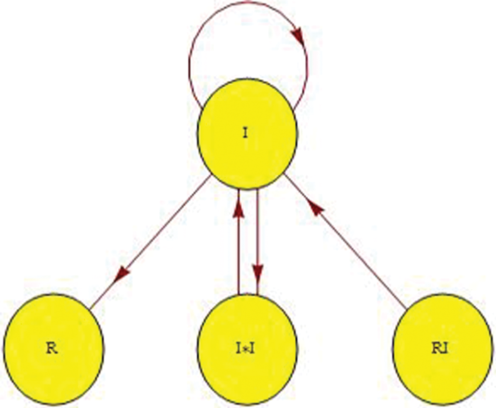
Figure 1: Proposition signal flow graph of the model
For the purposes of this discussion, let  be infected individuals who are carrying the virus, and
  be recovered individuals. Let
  represents susceptible individuals, and
  represents the physical contact number between susceptible and infected individuals. Then the model can be written in the following form [17,19]:
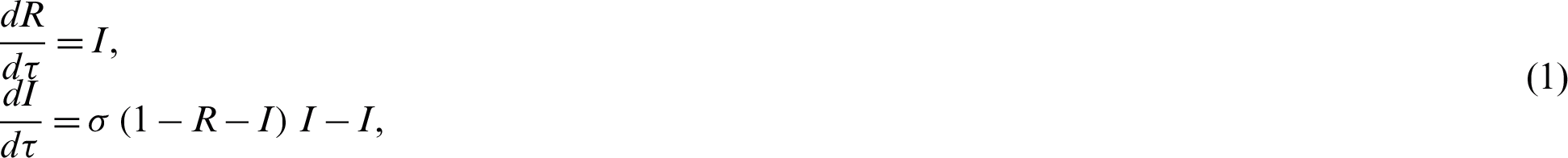
together with 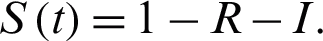 Let
Let 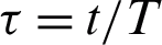 where t represents the time in days, and T represents the time of transmission of the virus which changes from 2–4 weeks. At the start of the outbreak in day t = 0, we consider the initial number of infected people is
  , and the initial recovered people is
2 The Equilibrium Point and Stability of Nonlinear COVID-19 Model
This section discusses the equilibrium point and the stability of the nonlinear COVID-19 model (1).
This subsection examines the equilibrium points of the nonlinear COVID-19 model. The model has two equilibrium points. For more insights regarding the dynamical behaviors system see [20]. Thus, by solving the next equations, the equilibrium points can be decided.
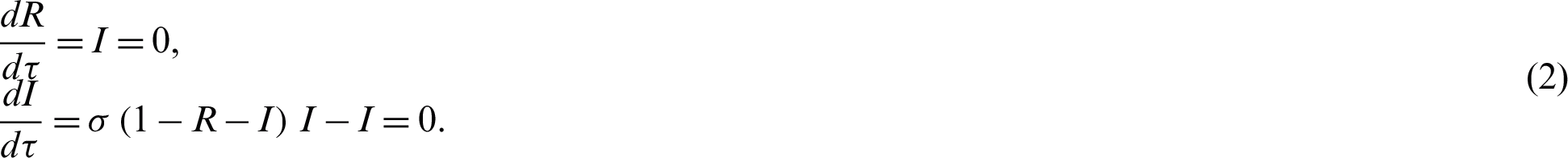
This System (2) has two equilibrium points:  and
and 
2.2 Studying the Stability of the Two Fixed Point
We calculate the Jacobian matrix for the Model (1) as follows:

To study the stability of System (2), we need to study the stability of Eq. (2).
 The Jacobian matrix
  for Model (1) is given by

Consequently, we have

Then, the eigenvalues are given by

the solution is stable if 
 The Jacobian matrix
  for model (1) is given by

Consequently, we have

then, the eigenvalues are given by

the solution is stable if 
2.3 Existence of Uniformly Stable Solution
This subsection explores the existence of uniformly stable solution. Let us define

Let  .
.
We have, at 


where  , and k4 are positive constants. It is suggested that every one of both capacities f1 and f2 agree with the Lipschitz condition as the two functions are absolutely continuous. For more information on the existence and uniqueness, see [13,14,20].
The signal flow graph is becoming more widely used since it empowers us with the flexibility to construct and develop the electronic circuits for dynamical frameworks. It can be utilized to delineate signals between the factors of the framework. In this section, the analysis is based upon a signal flow graph that is used to describe the COVID-19 model. More detailed discussion on the diagram theory can be found in [12–14,21]. The constructed adjacency matrix empowers us to determine all eigenvalues and the associated eigenvectors.
Fig. 1 shows the sign flow diagram  of the framework in which every vertex communicate with the condition of the framework. There is an edge
  if the state v1 directly affects the state v2.
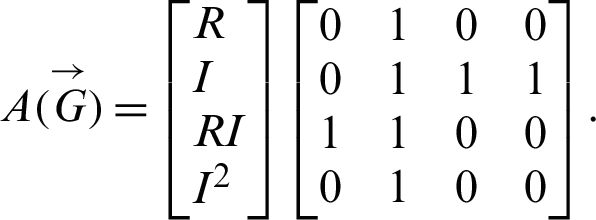
In this manner, the contiguousness grid  is as per the following:
 Adjacency matrix: The signal flow graph of the system has the following adjacency matrix
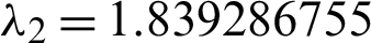
 Eigenvalues: The above matrix has four eigenvalues, namely
 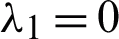 ,
, 

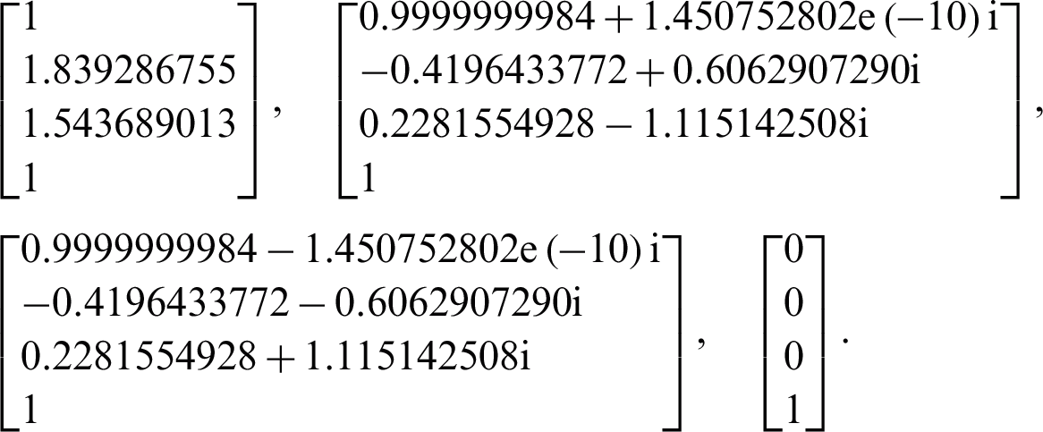
 Eigenvectors: The corresponding eigenvectors to these eigenvalues are easily found to be
Which can help study the topological structure of the mode see [9,13].
4 HPM Approximates the Solution for Nonlinear COVID-19 Model
This section presents the analytic approximate solution to the nonlinear COVID-19 (1). By using HPM technique [22,23], we construct a homotopy  , which satisfies:


According to the HPM technique, we suppose the solutions of Eqs. (8) and (9) as a power series in p, where p is the embedding small parameter:


Substituting Eqs. (10) and (11) into Eqs. (8) and (9), collecting the coefficients p, after some calculations we obtain:
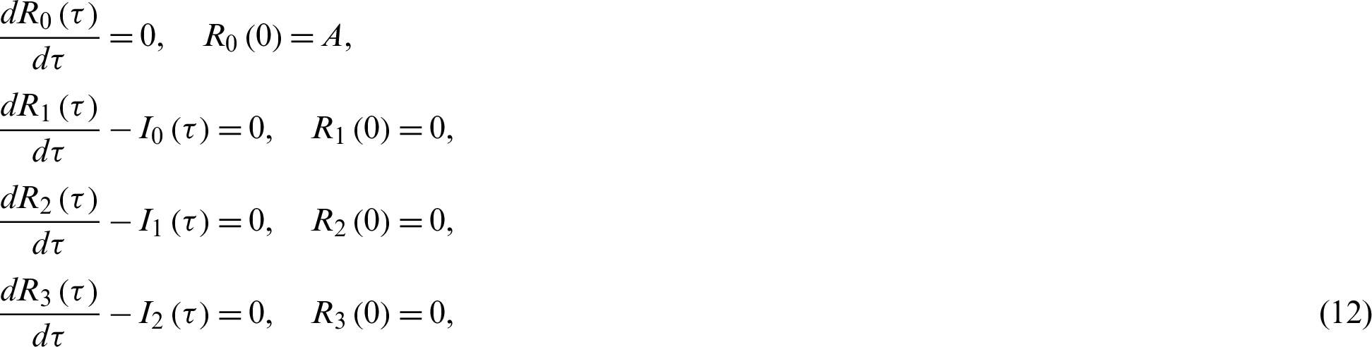
and
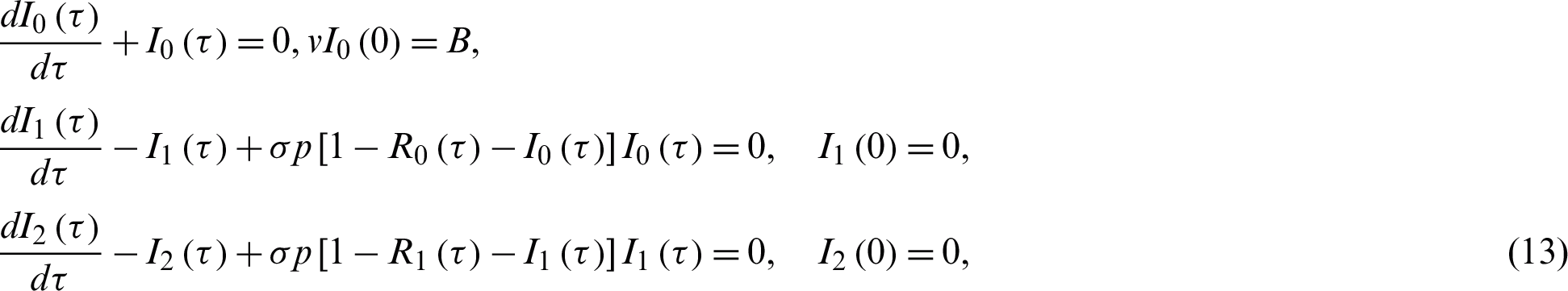
and so on. The above system of differential Eqs. (12) and (13) has the following solutions:
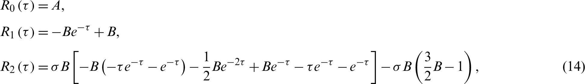
and
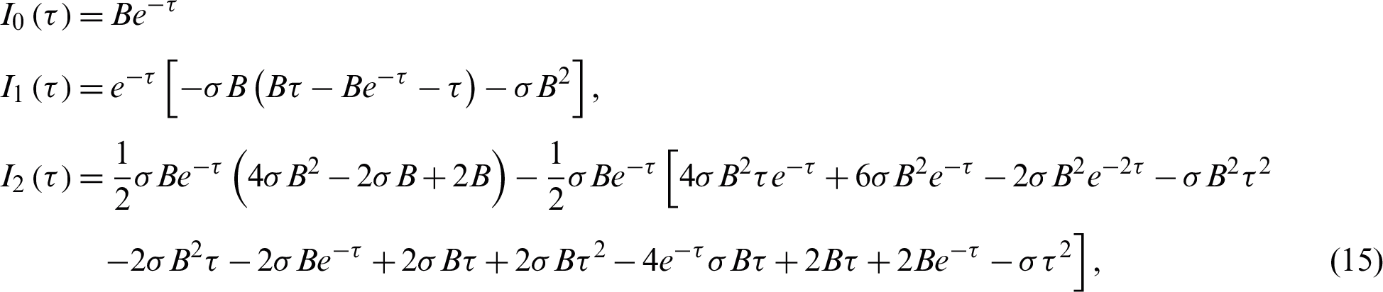
and so on. If  the analytic approximate solution takes the following form:

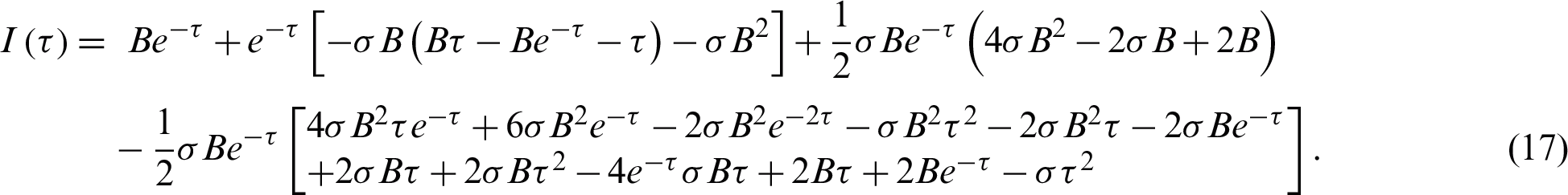
Figs. 2–5 discuss the behavior of the approximate solution (16) and (17), where A = 0.001 and B = 0.01.
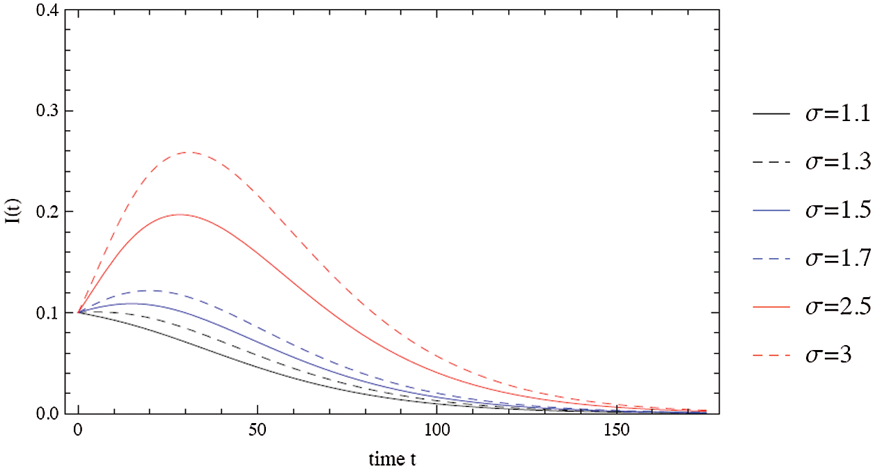
Figure 2: The evolution of the outbreak depends on the contact number 
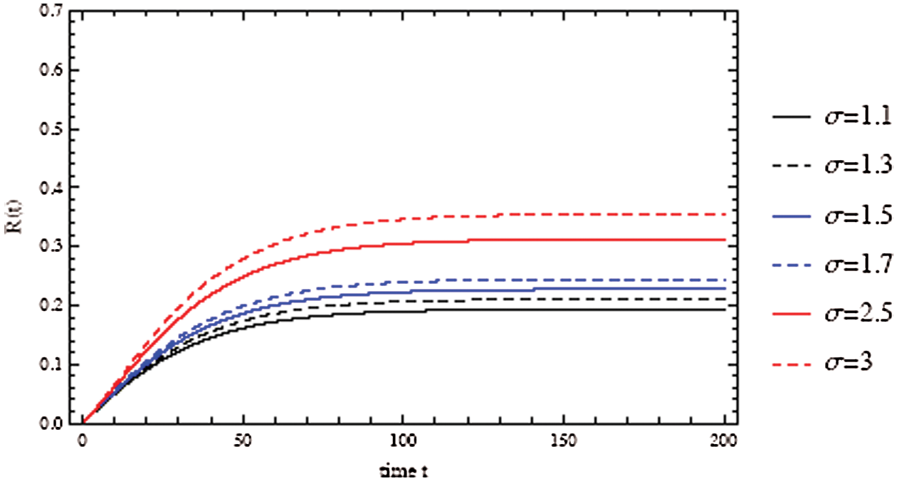
Figure 3: Solutions of the COVID-19 model over 200 days with an initial recovered individuals of 0. The recovered fractions as a function of time t
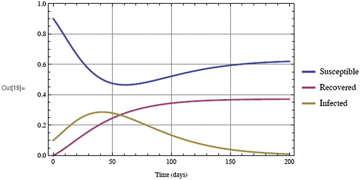
Figure 4: Solutions of the COVID-19 model over 200 days with an initial infected individuals of 0.1, an initial recovered individuals of 0, and a contact rate  of 3
of 3
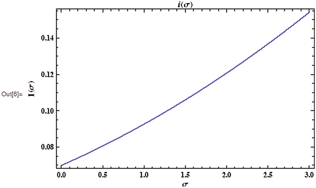
Figure 5: Evolution of the asymptotic fraction of infected individuals as a function of contact number 
5 RDTM Method Approximates the Solution for Nonlinear COVID-19 Model
In this section, we study the approximate solution to the nonlinear coronavirus Model (1) which is subject to the initial conditions at the beginning of the outbreak  and
and  Applying the RDT technique [24–29], we obtain the following iteration relations:
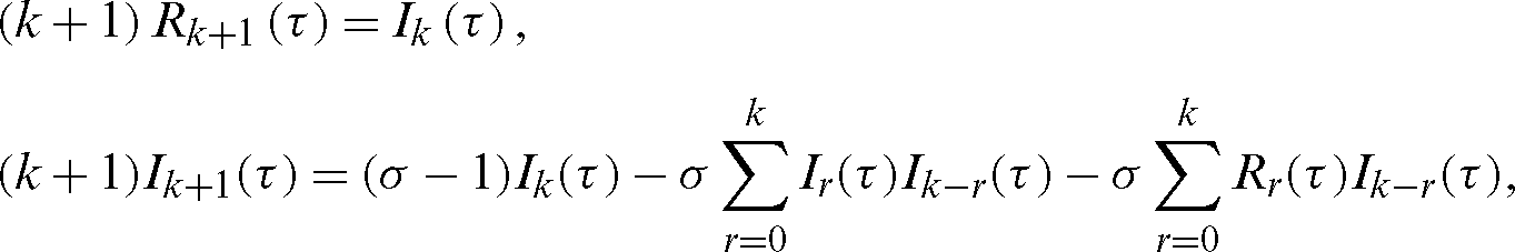
or
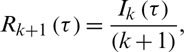
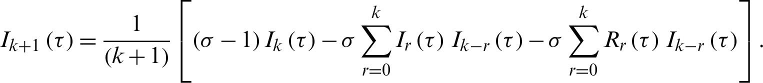
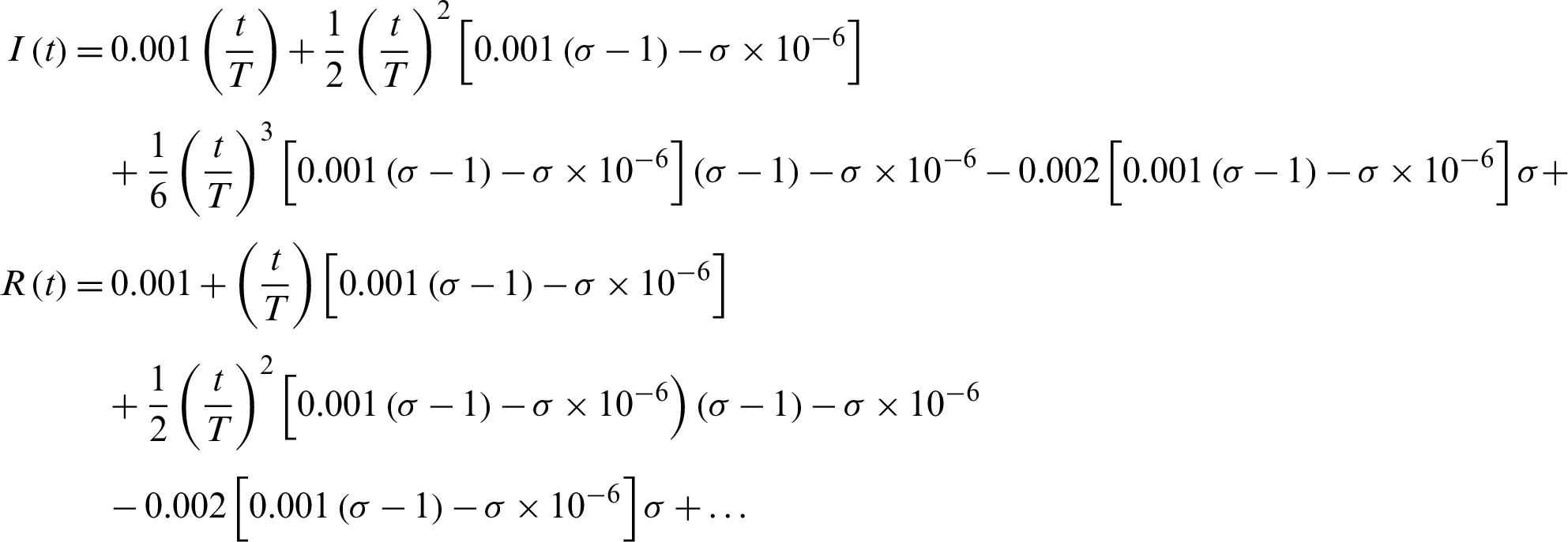
Finally, the differential inverse transforms are given by:

Consequently, after some calculations we get the approximate series solutions as
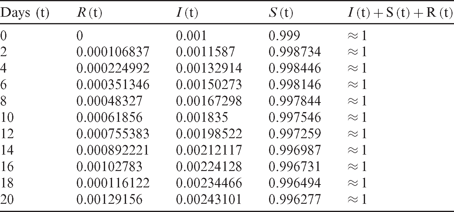
Tab. 1 shows how the number of susceptible, infected, and recovered individuals changes over 20 days.
Table 1: Outbreak of the COVID-19 over 20 days. The initial infected people is 10−3, the initial recovered people is 0, the transmission rate  is 2.5
6 Numerical Simulations and Discussion
This section presents numerical simulations to illustrate the key aspects of the development of analysis of COVID-19. Figs. 2–4 illustrate a typical scenario for the dynamical behavior of COVID-19. The spread of the virus grows exponentially until much of the population is infected or recovered, at which point the risk of infections begins to decline. Fig. 2 shows that the risk of spreading the virus depends on the contact number  between susceptible and infected people. It is clear that as the contact number
  increases; the proportion of infected people increases rapidly, resulting in a decreasing number of susceptible populations (Fig. 3). The importance of physical distance can be understood by reducing the contact number between susceptible and infected people from
  to
to 
As shown in Fig. 3, the coronavirus outbreak could reach its peak on around day 35–40, with almost 28% of the population infected, while 20% of the population recovered from the disease. Most importantly, it is obvious that towards the end of the epidemic, around 60 % of people remain susceptible, this means the susceptible people escaping from contracting infectious diseases and the COVID-19 has died out before everyone in the population has contracted it. Figs. 5 and 6 represent respectively, the evolution of the asymptotic fraction of infected and recovered individuals as a function of physical contact number  .
.
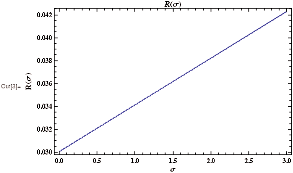
Figure 6: Evolution of the asymptotic fraction of recovered individuals after as a function of contact number 
This article explores the behavior of COVID-19 model by using the homotopy perturbation and modified reduced differential transform methods. The free disease equilibrium and stability point for the COVID-19 model are discussed. The model is described by a novel signal flow chart. Through our mathematical studies, the severity of the virus is clarified, which shows more influence by increasing the contact number. The numerical simulations demonstrate that the close connect between susceptible and infectious individuals is a major risk factor for spreading the virus while maintaining physical distance is essential to reduce the risk of spreading the virus.
Acknowledgement: The authors are thankful of the Taif University. Taif University researchers supporting Project No. (TURSP-2020/16), Taif University, Taif, Saudi Arabia.
Funding Statement: This paper was funded by “Taif University Researchers Supporting Project Number (TURSP-2020/16), Taif University, Taif, Saudi Arabia.”
Conflicts of Interest: Submitting authors are responsible for co-authors declaring their interests.
References
1. C. I. Siettos and L. Russo. (2013). “Mathematical modeling of infectious disease dynamics,” Virulence, vol. 4, no. 4, pp. 295–306.
2. S. M. Jenness, S. M. Goodreau and M. Morris. (2018). “Epimodel: An R package for mathematical modeling of infectious disease over networks,” Journal of Statistical Software, vol. 84, pp. 1–56.
3. O. Angulo, F. Milner and L. Sega. (2013). “A sir epidemic model structured by immunological variables,” Journal of Biological Systems, vol. 21, no. 4, 1340013.
4. F. Castiglione, F. Pappalardo, C. Bianca, G. Russo and S. Motta. (2014). “Modeling biology spanning different scales: An open challenge,” BioMed Research International, vol. 2014, no. 1–4, pp. 1–9.
5. H. M. M. Alotaibi. (2017). “Developing multiscale methodologies for computational fluid mechanics,” Ph. D. Thesis.
6. A. S. Shaikh, I. N. Shaikh and K. S. Nisar. (2020). “A mathematical model of COVID-19 using fractional derivative: Outbreak in India with dynamics of transmission and control,” Advances in Difference Equations, vol. 373, pp. 1–19.
7. A. S. Shaikh, V. S. Jadhav, M. G. Timol, K. S. Nisar and I. Khan. (2020). “Analysis of the COVID-19 pandemic spreading in India by an epidemiological model and fractional differential operator,” Preprints, pp. 2020050266.
8. M. Naveed, M. Rafiq, A. Raza, N. Ahmed and I. Khan. (2020). “Mathematical analysis of novel coronavirus (2019-ncov) delay pandemic model,” Computers, Materials & Continua, vol. 64, no. 3, pp. 1401–1414.
9. A. M. S. Mahdy and M. Higazy. (2019). “Numerical different methods for solving the nonlinear biochemical reaction model,” International Journal of Applied and Computational Mathematics, vol. 5, no. 6, pp. 1–17.
10. A. M. S. Mahdy. (2018). “Numerical studies for solving fractional integro-differential equations,” Journal of Ocean Engineering and Science, vol. 3, no. 2, pp. 127–132. [Google Scholar]
11. Y. A. Amer, A. M. S. Mahdy and E. S. M. Youssef. (2018). “Solving fractional integro-differential equations by using sumudu transform method and Hermite spectral collocation method,” Computers, Materials & Continua, vol. 54, no. 2, pp. 161–180. [Google Scholar]
12. K. A. Gepreel, M. Higazy and A. M. S. Mahdy. (2020). “Optimal control, signal flow graph, and system electronic circuit realization for nonlinear Anopheles Mosquito model,” International Journal of Modern Physics C, vol. 31, no. 9, pp. 1–18. [Google Scholar]
13. A. M. S. Mahdy, H. Higazy, K. A. Gepreel and A. A. A. El-dahdouh. (2020). “Optimal control and bifurcation diagram for a model nonlinear fractional SIRC,” Alexandria Engineering Journal, vol. 59, no. 5, pp. 1–21. [Google Scholar]
14. A. M. S. Mahdy, N. Sweilam and H. Higazy. (2020). “Approximate solution for solving nonlinear fractional order smoking model,” Alexandria Engineering Journal, vol. 59, no. 2, pp. 739–752. [Google Scholar]
15. M. A. Khan and A. Atangana. (2020). “Modeling the dynamics of novel coronavirus (2019-ncov) with fractional derivative,” Alexandria Engineering Journal, vol. 59, no. 4, pp. 2379–2389. [Google Scholar]
16. J. Li and X. Zou. (2009). “Modeling spatial spread of infectious diseases with a fixed latent period in a spatially continuous domain,” Bulletin of Mathematical Biology, vol. 71, no. 8, pp. 20–48. [Google Scholar]
17. J. G. De Abajo. (2020). “Simple mathematics on COVID-19 expansion,” MedRxiv. [Google Scholar]
18. T. M. Chen, J. Rui, Q. P. Wang, Z. Y. Zhao, J. A. Cui et al. (2020). “A mathematical model for simulating the phase-based transmissibility of a novel coronavirus,” Infectious Diseases of Poverty, vol. 9, no. 1, pp. 1–8. [Google Scholar]
19. W. O. Kermack and A. G. McKendrick. (1927). “A contribution to the mathematical theory of epidemics,” In Proc. of the Royal Society of London, Series A Containing Papers of a Mathematical and Physical Character, vol. 115, no. 772, pp. 700–721. [Google Scholar]
20. H. El-Saka. (2014). “The fractional-order sis epidemic model with variable population size,” Journal of the Egyptian Mathematical Society, vol. 22, no. 1, pp. 50–54. [Google Scholar]
21. R. Balakrishnan and K. Ranganathan. (2012). A textbook of graph theory. 1 ed. New York: Springer Science & Business Media. [Google Scholar]
22. J. H. He. (2006). “Homotopy perturbation method for solving boundary value problems,” Physics Letters A, vol. 350, no. 1–2, pp. 87–88. [Google Scholar]
23. K. A. Gepreel. (2011). “The homotopy perturbation method applied to the nonlinear fractional Kolmogorov-Petrovskii-Piskunov equations,” Applied Mathematics Letters, vol. 24, no. 8, pp. 1428–1434. [Google Scholar]
24. K. A. Gepreel, A. M. S. Mahdy, M. S. Mohamed and A. Al-Amiri. (2019). “Reduced differential transform method for solving nonlinear biomathematics models,” Computers, Materials & Continua, vol. 61, no. 3, pp. 979–994. [Google Scholar]
25. Y. Keskin and G. Oturanc. (2009). “Reduced differential transform method for partial differential equations,” International Journal of Nonlinear Sciences and Numerical Simulation, vol. 10, no. 6, pp. 741–750. [Google Scholar]
26. Y. Keskin and G. Oturanc. (2010). “Reduced differential transform method for generalized KDV equations,” Mathematical and Computational Applications, vol. 15, no. 3, pp. 382–393. [Google Scholar]
27. M. I. A. Othman and A. M. S. Mahdy. (2010). “Differential transformation method and variation iteration method for Cauchy reaction-diffusion problems,” Journal of Mathematics and Computer Science, vol. 1, no. 2, pp. 61–75. [Google Scholar]
28. Y. A. Amer, A. M. S. Mahdy and H. A. R. Namoos. (2018). “Reduced differential transform method for solving fractional-order biological systems,” Journal of Engineering and Applied Sciences, vol. 13, no. 20, pp. 8489–8493. [Google Scholar]
29. M. S. Mohamed and K. A. Gepreel. (2017). “Reduced differential transform method for nonlinear integral member of Kadomtsev-Petviashvili hierarchy differential equations,” Journal of the Egyptian Mathematical Society, vol. 25, no. 1, pp. 1–7. [Google Scholar]
 | This work is licensed under a Creative Commons Attribution 4.0 International License,, which permits unrestricted use, distribution, and reproduction in any medium, provided the original work is properly cited. |