Computers, Materials & Continua DOI:10.32604/cmc.2021.013390
Article

Classification of Fundus Images Based on Deep Learning for Detecting Eye Diseases

Nakhim Chea1 and Yunyoung Nam2,*

1Department of ICT Convergence Rehabilitation Engineering, Soonchunhyang University, Asan, 31538, Korea
2Department of Computer Science and Engineering, Soonchunhyang University, Asan, 31538, Korea
*Corresponding Author: Yunyoung Nam. Email: ynam@sch.ac.kr
Received: 05 August 2020; Accepted: 01 November 2020

Abstract: Various techniques to diagnose eye diseases such as diabetic retinopathy (DR), glaucoma (GLC), and age-related macular degeneration (AMD), are possible through deep learning algorithms. A few recent studies have examined a couple of major diseases and compared them with data from healthy subjects. However, multiple major eye diseases, such as DR, GLC, and AMD, could not be detected simultaneously by computer-aided systems to date. There were just high-performance-outcome researches on a pair of healthy and eye-diseased group, besides of four categories of fundus image classification. To have a better knowledge of multi-categorical classification of fundus photographs, we used optimal residual deep neural networks and effective image preprocessing techniques, such as shrinking the region of interest, iso-luminance plane contrast-limited adaptive histogram equalization, and data augmentation. Applying these to the classification of three eye diseases from currently available public datasets, we achieved peak and average accuracies of 91.16% and 85.79%, respectively. The specificities for images from the eyes of healthy, GLC, AMD, and DR patients were 90.06%, 99.63%, 99.82%, and 91.90%, respectively. The better specificity performances may alert patient in an early stage of eye diseases to prevent vision loss. This study presents a possible occurrence of a multi-categorical deep neural network technique that can be deemed as a successful pilot study of classification for the three most-common eye diseases and can be used for future assistive devices in computer-aided clinical applications.

Keywords: Multi-categorical classification; deep neural networks; glaucoma; age-related macular degeneration; diabetic retinopathy

1  Introduction

Diabetic retinopathy (DR), glaucoma (GLC), and age-related macular degeneration (AMD), the major causes of vision loss and blindness around the world are the focus of our study. DR is vision loss caused by diabetes mellitus, the most common cause of vision loss and blindness among adults [1,2]. From 2000 to 2030, the global diabetes population was estimated to grow from 2.8% (171 million) to 4.4% [3], with an additional 195 million people developing DR [4–6]. Almost all of the patients with type 1 diabetes and over 60% with type 2 diabetes were expected to develop DR in the next 20 years [7]. These diabetic patients were expected to account for 2% of blindnesses and 10% of vision losses in the next 15 years [8]. The patients reported have shown gradual growth but were expected to increase rapidly. According to a report, in the early 21st century, the incidence of diabetes mellitus has doubled in the United States and increased by a factor of three to five times in India, Indonesia, China, Korea, and Thailand [9]. DR prevailed in both developed and developing countries. The second most common cause of vision loss, GLC, is the effect of differential pressure in intraocular that damages the optic nerve head and causes vision loss. In 2000, 66.8 million people worldwide developed primary GLC; of these 6.7 million developed bilateral blindness [10]. This disease became the second leading cause of vision loss and blindness by 2010, accounting for about 60.5 million of the GLC patient population around the world [11]. It affected the size of optic nerve head in reshaping or damaged the origin of its optic nerve, both diagnosable in fundus photography images. The third most common cause of vision loss and blindness is AMD, which is an enormous threat in developed countries. Although DR and GLC were more prevalent, the incidence of AMD in people older than 60 years has grown and was reported alone to cause 8.7% of blindness worldwide, mostly in developed countries [12–20]. Those who suffered from AMD have surely encountered difficulties in their life due to the importance of vision, being one of the five basic human senses. Moreover, the optic nerve, the nerve of sight, is the second sensory and critical nerve among the twelve cranial nerves.

Various techniques are applied by experts or doctors to diagnose eye diseases; two typical ones are optical coherence tomography, which captures a cross-sectional image and fundus photography. Optical coherence tomography has played a major role in medical diagnoses not only of the eye but also of other organs, such as the brain. This technique’s cross-sectional images of the eye affected by DR, GLC, and AMD had been studied by many researchers, such as Hwang et al. [21], Bussel et al. [22], and Lee et al. [23]; however, the techniques had some disadvantages.

Fundus photography images the inner eye with a specialized camera and has been of significant interest to researchers. The same image can be used to detect several eye diseases, such as the three in this study. The various fundus photography techniques can be classified into three types: fluorescein angiographic, mydriatic, and non-mydriatic, which entail an examination of the retina and choroid or blood flow by fluorescent or indocyanine green dyes, by use of pupil dilation, and by imaging without dilation, respectively. In this study, fundus photographs from various open-source databases are to be combined to classify eye diseases.

The current study uses a feedforward neural network to detect several eye diseases using fundus photographs; we ensure that this study will play a leading role in future work. In the field of DR detection, many studies have used deep learning approaches, such as those by Qummar et al. [24] performed an ensemble approach to develop an automatic DR detection system for retinal images, and Mateen et al. [25] performed a combination of a Gaussian mixture model, Visual Geometry Group (VGG) networks, singular value decomposition, and principle component analysis to create a DR image classification system. In GLC detection, a few studies have used ensemble and neural network approaches; for instance, Singh et al. [26] created a deep learning ensemble with feature selection techniques for an automatic GLC diagnostic system. In AMD detection, a proposed computer-aided diagnosis system based on a custom convolutional neural network provided second opinions to assist ophthalmologists in the study by Tan et al. [27]. Researchers have published many papers relevant to computer-aided diagnosis that may offer tools to assist ophthalmologists in eye disease screening and detection.

This manuscript is organized as follows. Section 2 is a literature review of eye-disease classification. Section 3 describes our data acquisition. The preprocessing and processing techniques applied in the paper are described in Section 4. Section 5 is our classification results. A discussion and conclusion are given in Section 6.

2  Related Work

Many studies have played significant roles in leading experiments on eye disease detection using different types of approaches. In this study, we focused on classification using a deep convolutional neural network (DNN). The most common approaches to disease detection and screening using fundus photography were feature extraction with an ensemble, traditional machine learning, and DNN. As mentioned above, prior studies [24–27], provided possibilities for classifying eye diseases and thus for diagnosis. However, the current study emphasizes one approach, DNN, which has recently been studied by many researchers to provide the classification of multiple eye diseases.

Various neural networks, including novel, pre-trained convolutional, and meta-cognitive neural networks, have been deployed to diagnose eye diseases automatically. For screening DR, Gardner et al. [28] proposed a neural network diagnostic method with 88.40% sensitivity and 83.50% specificity; Banu et al. [29] proposed a novel meta-cognitive neural network, which monitored and controlled a cognitive neural network, yielded 100% accuracy, sensitivity, and specificity. This performance was obtained by eliminating the optic disc from fundus images using the techniques of “robust spatial kernel fuzzy c-means” before the meta-cognitive neural network classifier; the optic disc was one of the most significant features of GLC detection in this study. By contrast, Raghavendra et al. [30] proposed a support vector machine model for detecting GLC. Their method yielded maximum accuracy, sensitivity, and specificity of 93.62%, 87.50%, and 95.80%, respectively, over a public dataset using a 26-feature classification technique. Moreover, another study [31] proposed an 18-layer neural network model to detect GLC, which yielded accuracy, sensitivity, and specificity of 98.13%, 98.00%, and 98.30%, respectively; the technique was a major change from its neural network predecessors. The field of AMD detection is represented by two experimental studies. Lee et al. [23] proposed a method with a 21-layer neural network, that yielded accuracy, peak sensitivity, and peak specificity of 93.45%, 92.64%, and 93.69%, respectively; and Burlina et al. [32] proposed a pre-trained convolutional neural network model, that achieved peak accuracy, sensitivity, and specificity of 95.00%, 96.40%, and 95.60%, respectively.

A wide neural network would be able to detect multiple eye diseases automatically at the feedforward stage without overlapping classification results. Thus, it might be possible to diagnose these diseases more quickly and reduce their impacts in terms of vision loss and blindness. Choi et al. [33] used a deep neural network (VGG-19) in their pilot studies. Three-class early disease screening among normal retina (NR), background DR, and dry AMD showed a peak accuracy of 72.8% via the technique of transfer learning with a random forest when applied to images from the Structured Analysis of the Retina (STARE) database. Moreover, five-class eye-disease classification, NR, background DR, proliferative DR, dry AMD, and wet AMD, achieved a peak accuracy of 59.1% with the same model structure. For a small database, this performance was not a promising result. However, this leading study confirmed that it might be possible to achieve an acceptable result with a 19-layer neural network analyzing a 397-file database of 14 disease categories. The reported performances of wide neural networks inspired the current investigation of this promising possibility for multi-eye-disease detection via a deeper pre-trained neural network applied to the public datasets currently available online.

3  Materials

3.1 Research Scope

This study uses databases that are currently openly available to investigate the problem of multi-class classification to prevent vision loss and blindness. Despite there being other types of eye diseases, e.g., hypertensive and radiation retinopathies; only the three most common eye diseases, DR, GLC, and AMD, are considered in this research. The datasets had similar properties: field of view ranging from to , specialized digital fundus photographs that had already been labelled by experts, and consideration of the three eye diseases of interest.

3.2 Retinal Fundus Image Datasets

A total of 2335 retinal fundus images, NR: 1195, GLC: 168, AMD: 65, DR: 907, were obtained for this study from 5 databases, as follows. Each image used had been annotated by a named expert associated with the database of which it was a part.

The Online Retinal Fundus Image Database for Glaucoma Analysis and Research (ORIGA) database, stylized by its authors as “ORIGAlight,” contained 650 images, comprising 168 GLC and 482 randomly selected non-GLC images, from the Singapore Malay Eye Study. That study examined 3280 Malay adults aged 40 to 80 years, of whom149 were GLC patients. Image acquired at a resolution of and [34]. Fig. 1 shows some sample images from this database.

Figure 1: Random images from the online retinal fundus image database for glaucoma analysis and research (ORIGA) database

The Indian Diabetic Retinopathy Image Dataset (IDRiD) database contained 516 images, comprising 168 non-DR and 348 DR training and testing images annotated in a file with a comma-separated value format. The images were acquired using a digital fundus camera (model: Kowa, VX-10 alpha) with a field of view, centered near to the macula and a resolution of pixels. Images were stored in the Joint Photographic Experts Group (JPG) file format, and the file size was 800 kB. In total, 166 NR images and 254 DR images, all clearly annotated, were selected for use [35]. Fig. 2 shows some sample images from this database.

Figure 2: Random images from the Indian Diabetic Retinopathy Image Dataset (IDRiD) database

The Methods to Evaluate Segmentation and Indexing Techniques in the field of Retinal Ophthalmology database (known by its French acronym, MESSIDOR) consisted of 1200 fundus color images classified in folders, comprising 547 non-DR and 653 DR images. The later were classified into three levels of eye disease: mild (153 images), moderate (246 images), and severe DR (the remainder). The images captured by three separate charge-coupled devices (3CCD) mounted on a Topcon TRC NW6 camera to form a non-mydriatic fundus retinography with a field of view using eight bits per color plane at a resolution of , , or pixels [36]. Eight hundred of the images were acquired with pupil dilation (one drop of tropicamide at 0.5%) and 400 without dilation. Fig. 3 shows some sample images from this database.

Figure 3: Random images from the methods to evaluate segmentation and indexing techniques in the field of retinal ophthalmology (MESSIDOR) database

The Automated Retinal Image Analysis (ARIA) database consisted of 143 images from adults: 23 with AMD, 59 with DR, and 61 with a control group. The images were acquired in color by using a fundus camera (model: Zeiss, FF450+) with a field width, and were stored as uncompressed files in the Tagged Image File Format (TIFF) format [37,38]. We used all 23 AMD images from this database. Fig. 4 shows some sample images from this database.

Figure 4: Random images from the Automated Retinal Image Analysis (ARIA) database

The Structured Analysis of the Retina (STARE) project was initiated in 1975 comprising 397 images in an annotated file. These images were acquired using a fundus camera (model: Topcon, TRV-50) with a field of view and subsequently digitized at a resolution of pixels, with 24 bits per pixel, “standard red-green-blue (RGB) color space” [39,40]. Forty-two images with AMD annotation were selected for our AMD training and testing dataset. Fig. 5 shows some sample images from this database.

Figure 5: Random images from the Structured Analysis of the Retina (STARE) database

3.3 Full Combined Dataset (NOISE-STRESS)

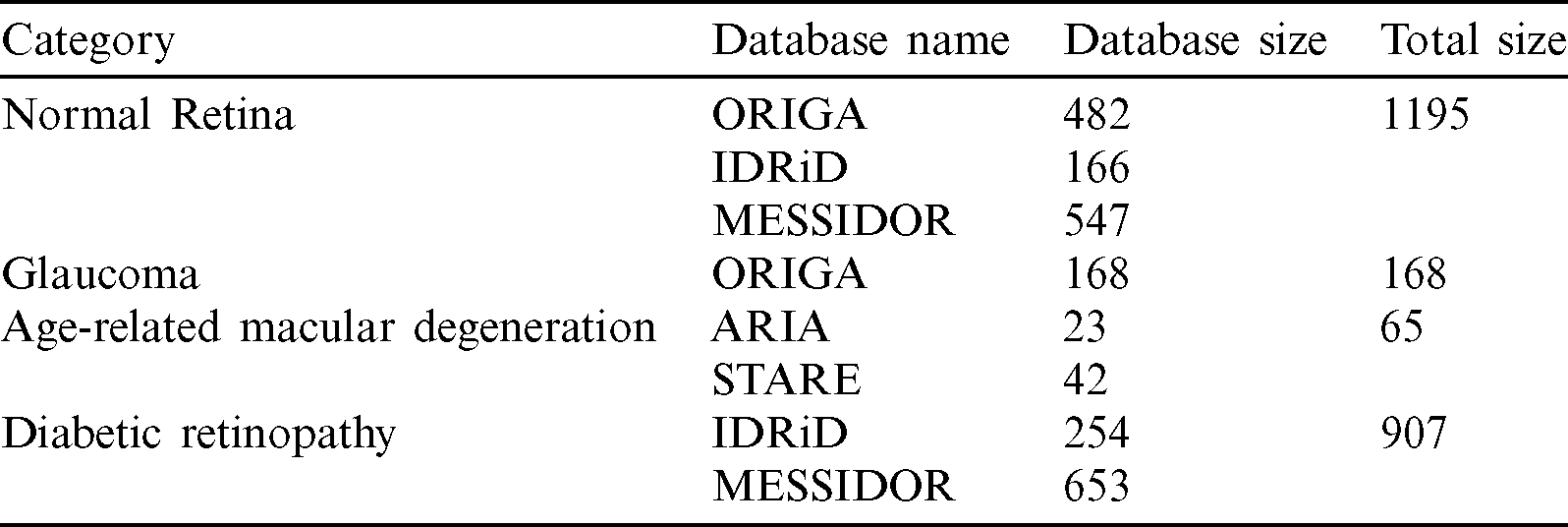
Our full dataset, which was called NOISE-STRESS, consisting of the selected images from the five public datasets, contained a total of 2335 retinal fundus images: 1195 NR, 168 GLC, 65 AMD, and 907 DR. The ORIGAlight, IDRiD, MESSIDOR, ARIA, and STARE datasets provided 650, 420, 1200, 23, and 42 of these images, respectively. The ORIGAlight NR images were included for a noise experiment test. Some of the 61 control group images from the ARIA database and some of the NR group images from the STARE database were excluded. Tab. 1 summarizes the full combined dataset.

Table 1: Full combined dataset (NOISE-STRESS)

3.4 Mild and Moderate-DR Omission Dataset (NOISE)

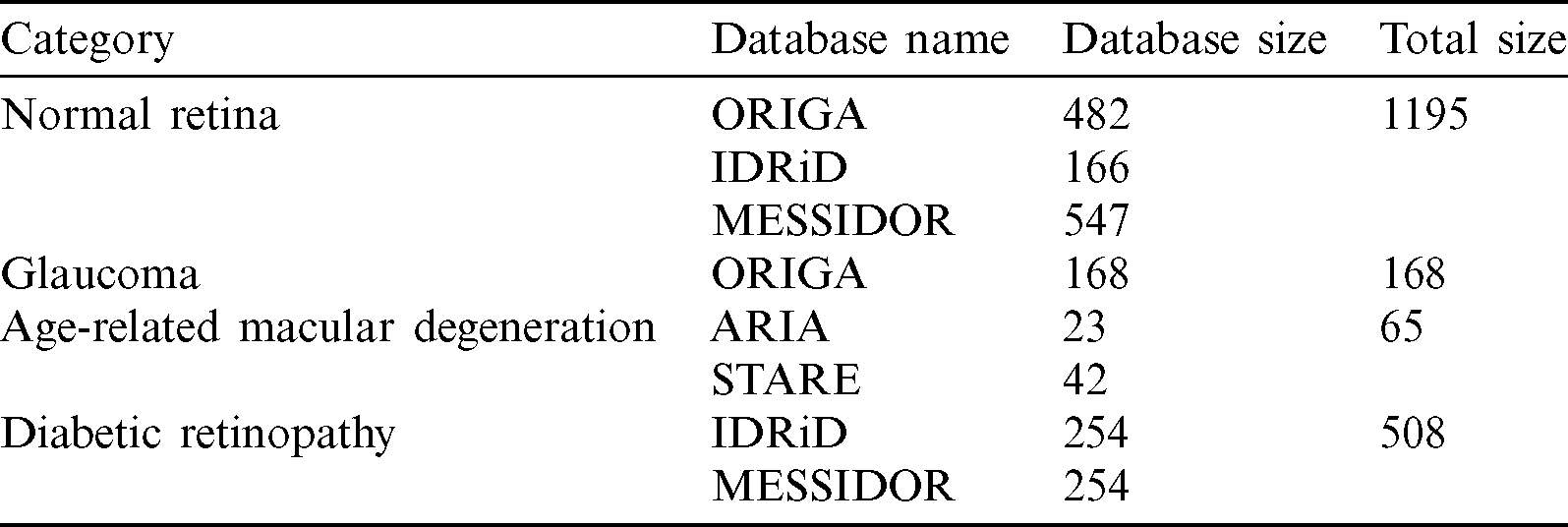
From the full NOISE-STRESS data, a dataset that we called NOISE was selected by excluding the mild and moderate DR images from the MESSIDOR database, leaving a total of 1936 retinal fundus images: NR, GLC, AMD, and DR of 1195, 168, 65, and 508 images, respectively. The ORIGAlight, IDRiD, MESSIDOR, ARIA, and STARE datasets were the sources of 650, 420, 801, 23, and 42 of these images, respectively. The ORIGAlight NR images were included for a noise experiment to determine if the nodes of the NOISE-STRESS dataset classification neural networks could be fooled into giving the wrong diagnosis. Tab. 2 shows the summary of mild and moderate-DR omission dataset.

Table 2: Mild and moderate-DR omission dataset (NOISE)

3.5 Non-Glaucoma Omission Dataset (STRESS)

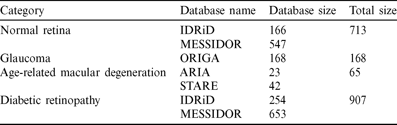
From the NOISE-STRESS dataset, a dataset that we called STRESS was formed by removing the noise images in ORIGAlight database comprising a total of 1853 retinal fundus images: 713 NR, 168 GLC, 65 AMD, and 907 DR images. The ORIGAlight, IDRiD, MESSIDOR, ARIA, and STARE datasets were the sources of 650, 420, 801, 23, and 42 of these images, respectively. The NR images from ORIGAlight were excluded. Tab. 3 shows the summary of the non-glaucoma omission dataset.

Table 3: Non-glaucoma omission dataset (STRESS)

4  Methods

Automatic categorization of the three most common retinal fundus diseases will significantly assist ophthalmologists in early, low-cost eye disease detection. The proposed method has two stages: the data preprocessing and retinal image categorization (training and testing phases). Fig. 6 shows the proposed approach. First, each dataset was preprocessed by the following stages, the shrinking region of interest, iso-luminance plane contrast limited adaptive histogram equalization, k-fold cross-validation, and data augmentation. Second, each training set resulted from the preprocessing stage proceeded with training settings to create a learnt weight for each dataset. Finally, each testing set was predicted by the learnt weight created in the training phase to provide the testing results of eye-disease classifications.

Figure 6: Eye disease evaluation process

4.1 Pre-Processing

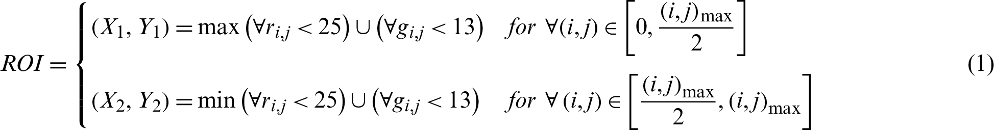
Before training our model, we applied a few methods of image normalization. Various researchers had had different approaches to their image preprocessing. In this paper, we shrank the region of interest of the original fundus images to standardize them across the datasets. This was done automatically, with thresholds of 25 and 13 for the red and green channels, respectively, while the blue channel was a complementary layer. The coordinates for shrinking the region of interest are expressed, where imax and jmax are the image width and height, as follows:

We also applied another preprocessing technique, a technique that we called ISOL-CLAHE. ISOL-CLAHE is a process of contrast limited adaptive histogram equalization (CLAHE) applying on an isoluminant plane. According to Han et al. [41], we modified this technique for our retinal fundus images within an isoluminant plane. Histogram equalization on the isoluminant plane improved the lowest mean absolute error rate from the linear cumulative distribution function among previous studies on separate RGB histogram equalization [41–43]. All of the original image files (located in four parent directories, NR, GLC, AMD, and DR, and eight child subdirectories) underwent three-dimensional CLAHE. The images were converted to a color space specified by the International Commission on Illumination (known by its French acronym, CIELAB) to extract lightness using software from an open-source library [44]. CLAHE with a clip limit of 1.5 and slicing grid kernel size of eight was followed by resizing to pixels. Fig. 7 indicates the implementation of ROI shrink and ISOL-CLAHE.

Figure 7: Shrinking region of interest (ROI) and isoluminant-plane contrast limited adaptive histogram equalization (ISOL-CLAHE). (a) The original image with its original size. (b) The ROI shrinking image. (c) The ISOL-CLAHE image

K-fold cross-validation in its tenfold variety performed better than leave-one-out, twofold, and fivefold cross-validation in models with a larger number of features, according to Breiman et al. [45]. Ron Kohavi [46] reported that stratified tenfold cross-validation performed better than twofold and fivefold cross-validation, or bootstrapping with a lower variance but an extremely large bias. In the current study, we used stratified tenfold cross-validation for the fundus image classification with data shuffling to prevent bias from the data preparation, as introduced by [47]. The full dataset was divided into three parts comprising 80%, 10%, and 10% of the images for experimental training, validating, and testing, respectively.

One technique to enlarge datasets without generating fake images is called data augmentation. The collected dataset had various numbers of images in each disease type. At random, a transformation was applied to an image, such as an rotation, a 25% change in brightness, a 20% magnification, and a horizontal reflection. This created a balanced training and testing dataset of up to 9400 images for the full combined dataset experiment preventing differences in performance because there were very few AMD images but many NR and DR ones. We did not use some typical transformations, such as shear, or height or width shifts in the data augmentation method. Typically, the fundus image was taken by an ophthalmologist from a direction in front of the participant. Thus, shear range might not be an option in this procedure. Similarly, the fundus image should contain every feature that occurred naturally, such as an optic disc, a macula, and blood vessels; hence, we did not apply, because it might cause an unintentional loss of one of these features. Some examples of data augmentation on a MESSIDOR dataset are shown in Fig. 8.

Figure 8: Illustrations of data augmentation from a MESSIDOR image-set. (a) The original image from ISOL-CLAHE. (b) An augmented image with +25% brightness and rotation. (c) An augmented image with +25% brightness, 20% zoom-out, horizontal flip, and rotation. (d) An augmented image with 25% brightness, 20% zoom-in, horizontal flip, and rotation

4.2 Model Architectures and Settings

Residual Networks (ResNets) were deep neural networks named for their residual state [48]. This type of network took a leap over unnecessary convolutional layer blocks using a shortcut connection [49]. We utilized three residual network (ResNet) architectures such as ResNet-50, ResNet-101, and ResNet-152, comprising 50, 101, 152 weight layers with 25, 610, 216, 44, 654, 504, and 60, 344, 232 total number of parameters, respectively. The original input and output shape of these models were 3 and 1,000 fully connected Softmax regression classes. We modified the input shape to an optimal shape of 3 for this study, while the output was a four-class fully connected Softmax regression prediction probability.

Visual geometry group proposed networks that the twos, VGG-16 and VGG-19, consisted of 16 and 19 weight layers with total numbers of parameters of 138 million and 144 million, respectively [50]. The original input and output shapes, and the modified ones we used in the current study, were identical to those of ResNets.

Neural network optimizers played important roles in selecting and fine-tuning these weights to overcome the most accurate possible form, with loss functions guiding the optimizers to move in the right direction. An adaptive gradient extension optimizer (Adadelta) improved the learning robustness and learning rate variation [48] compared to the predecessor adaptive gradient algorithm optimizer. Zeiler [51] reported that this optimizer had the lowest test error rate among various competitors, including stochastic gradient descent and momentum optimizers. We used an adaptive gradient extension optimizer with a learning rate of 0.001 and categorical cross-entropy loss function.

Several techniques were available to prevent overfitting of the network. One efficient technique was early-stopping, which works by monitoring the validation error rate during training and terminating that process if the validation error did not improve after a certain number of epochs, called “patience” [48]. An optimal drop-out rate could determine the possibility of overfitting. The combination of early-stopping and drop-out rate optimization was proposed by Gal et al. [52] to achieve a smaller test error rate. In the current study, we used an early-stopping function with a minimum increment for the validation-loss of 0.001, a patience of 20 epochs, and a dropout rate of 0.05 for the optimal prevention of overfitting.

To perform the classification, we employed the TensorFlow [53] and Scikit-Learn [54] software to train and evaluate the proposed architectural deep neural network models. We executed the technique on our system configuration of a dual-core set up as follows: 2 Intel Xeon Silver 4114 CPUs@2.2 GHz, GB DIMM DDR4 Synchronous RAMs@2400 MHz, GB Samsung 970 NVMe M.2 SSDs, and 3 NVIDIA TITAN RTX GPUs 24 GB GDDR6@1770 MHz-4608 Compute Unified Device Architecture (CUDA) cores.

5  Results

5.1 Full Combined Dataset (NOISE-STRESS) Test Result

After the process of comparing the four-class eye-disease classification system using different DNN model architectures, we obtained interesting performance data on data augmentation using a ResNet with a depth of 50-layer layers. As we mentioned above, the NOISE-STRESS test dataset contained noise from non-GLC images. If a neural network outperformed the others, this was taken to indicate that it would be a great classifier for multi-class categorization. However, it might have performed so well by overfitting to the noise data, which would cause multi-class detection problems. With the 2335 original images, the ResNet-50 performed with average accuracy, sensitivities for NR, GLC, AMD, and DR of 73.12%, 77.06%, 18.13%, 53.33%, and 79.00%, respectively. Moreover, the specificities for these four classes were 70.45%, 98.74%, 99.73%, and 81.77%, respectively. With data augmentation, the ResNet-50 model achieved the highest accuracy compared to the VGG networks or their deeper siblings, the ResNet-101 and ResNet-152 models. With data augmentation, the ResNet-50 achieved an average accuracy of 76.71% and sensitivities for NR, GLC, AMD, and DR of 45.40%, 83.96%, 98.00%, and 79.49%, respectively. Additionally, the specificities of these four classes were 88.51%, 91.99%, 99.26%, and 89.19%, respectively. With these performance rates, it might be valid to assume that data augmentation of the datasets achieved generalization over the models. Tab. 4 shows the results of the NOISE-STRESS dataset test.

Table 4: Full combined dataset (NOISE-STRESS) test result

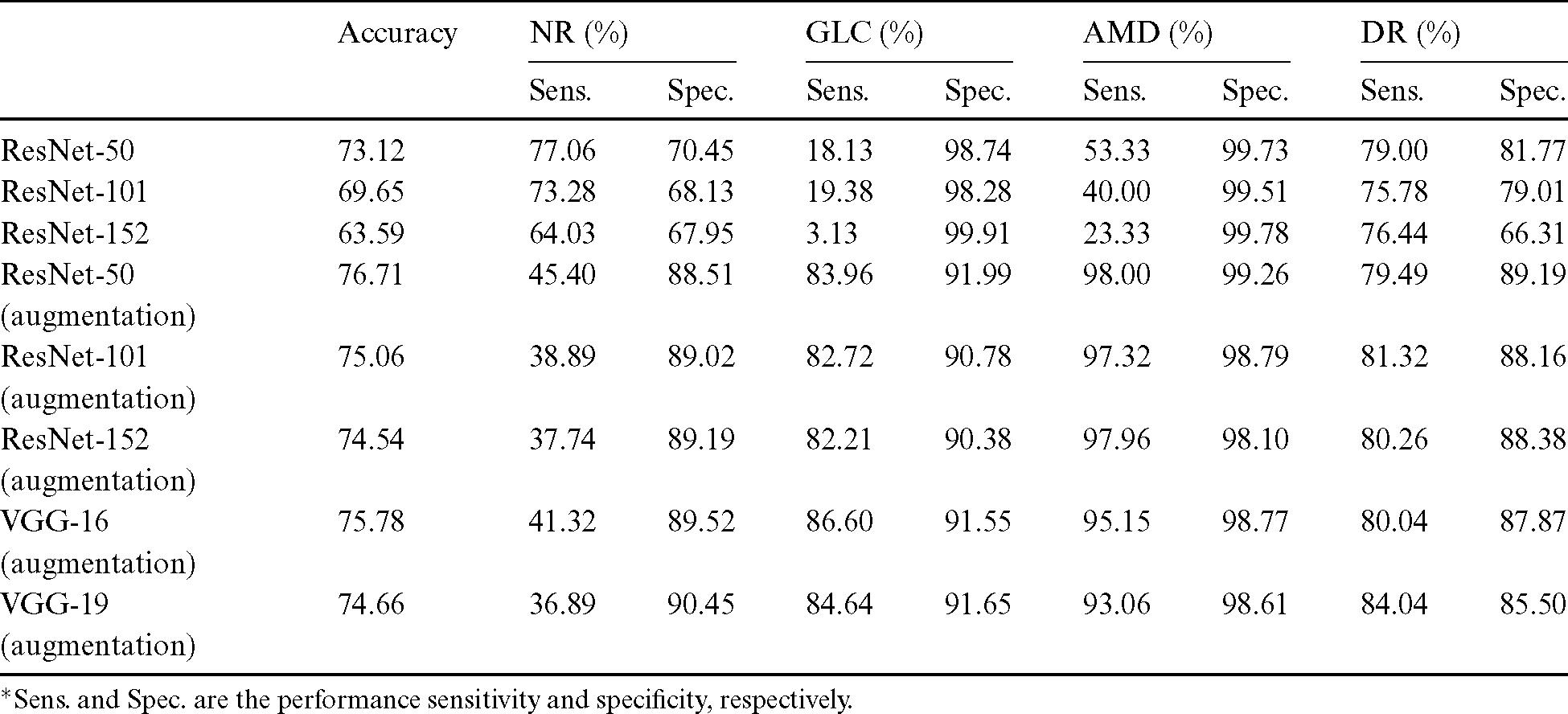
*Sens. and Spec. are the performance sensitivity and specificity, respectively.

5.2 Mild and Moderate-DR Omission Dataset (NOISE) Test Result

The results of testing with the NOISE dataset showed that the decrease in data improved the classification performance and generated a higher level of generalization for the detection models. The average accuracy was 80.27%, and the sensitivities for NR, GLC, AMD, and DR were 57.23%, 83.11%, 99.53%, and 81.19%, respectively. The specificities of these four classes were 89.21%, 92.03%, 99.02%, and 93.43%, respectively. The omission of mild and moderate DR images from the NOISE-STRESS dataset decreased the stress of information generalization across the DNN to produce higher performance. This test was an experiment using a neural network to see what happened with fewer stress data. Ordinarily, stress data prevails in the open-access dataset for DR and other disease types; hence, we included a STRESS result in this subsection incorporating those data. Tab. 5 shows the result of the NOISE-STRESS, NOISE, and STRESS dataset test.

Table 5: NOISE-STRESS, NOISE, and STRESS dataset test result

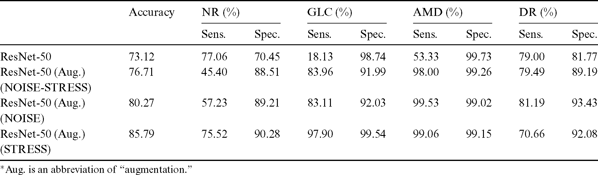
*Aug. is an abbreviation of “augmentation.”

5.3 Non-Glaucoma Omission Dataset (STRESS) Test Result

After excluding non-GLC images from the NOISE-STRESS dataset, average accuracy was 85.79%, and sensitivities of NR, GLC, AMD, and DR were 75.52%, 97.90%, 99.06%, and 70.66%, respectively, for the ResNet-50 model with data balancing. The specificities of the four classes were at the rate of 90.28%, 99.54%, 99.15%, and 92.08%, respectively. The better specificity performances compared to those with the NOISE-STRESS dataset suggests better caution for patients in the early stage of eye diseases.

The results from testing k-fold cross-validation of mild, moderate DR, and non-GLC omission dataset achieved a peak accuracy of 91.16% for the experiment of four-class eye-disease classification. The average accuracy from the 50-layer ResNet with tenfold cross-validation was 85.79%. Tab. 6 shows the results of testing various k-fold cross-validations with the STRESS dataset.

Table 6: Individual fold accuracy from STRESS dataset

6  Discussion and Conclusion

In the Results, Subsection 5.1, we observed that data augmentation not only played an important role in data generalization with a dataset, as noted by Perez et al. [55], in that validation accuracy was improved, but also resulted in remarkable testing performances with these fundus photographs. From the full combined testing dataset, we additionally observed that the combination of data augmentation with the ResNet-50 model resulted in better performance than that achieved by other competitive models for eye disease classification. In our opinion, the ResNet-50 model might distinguish the maximum number of features possible in the depth available from an image with a resolution of pixels. Moreover, the residual property of the networks might allow them to learn everything that could be learned with fundus images. Deeper residual models might obtain too many features in their nodes, which might cause slight overfitting.

We excluded the mild and moderate DR images from our training and testing dataset in Results, Subsection 5.2 so as to investigate the performance improvement resulted from using less stress data. The slight improvement with the NOISE dataset confirmed our hypothesis: the less challenging the data was, the higher the performances were. The previous experiment achieved an accuracy of 76.71%, whereas this experiment reached 80.27% accuracy, as we expected.

In our experimental sequence, we developed a dataset to test noise tolerance. As a result, we obtained 85.79% accuracy from the STRESS dataset (Result, Subsection 5.3). Of its total of 650 images, 482 were non-GLC images consisting of NR or non-GLC from ORIGAlight. In our experiment, the performance improved significantly after the exclusion of that 40% of noisy data from our NR data. Additionally, the stress inclusion of the mild and moderate DR images from the MESSIDOR dataset had a slight impact on overall performances, as we expected. For publicly available datasets, fundus photographs should undergo inter-rater reliability tests by both the experts employed by those databases and by local experts in order to improve the classification of multiple eye diseases.

We tested deep neural networks to classify fundus photographs with noisy and challenging data. Within a 50-layer ResNet architecture, our proposed method achieved 85.79% accuracy from the STRESS dataset using 10-fold cross-validation. A peak accuracy of 91.16% was obtained from this four-class eye disease classifier with our data preprocessing technique.

In conclusion, this study revealed that multi-category classification applied to public datasets could achieve a significant improvement in performance over previous studies, with changes to the preprocessing and data acquisition stages. In addition, this investigation showed the feasibility of multiple category diagnosis on multiple combined datasets. Thus, this can be judged as a successful pilot study of classification for the three most common eye diseases to develop assistive tools in the future for medical diagnosis. We also confirm that the publicly available fundus image databases may be inspired by valuable data for researchers who intend to deploy computer-aided systems for eye disease detection.

Funding Statement: This work was supported by the KIAT (Korea Institute for Advancement of Technology) grant funded by the Korea Government (MOTIE: Ministry of Trade Industry and Energy) (No. P0012724) and the Soonchunhyang University Research Fund.

Conflicts of Interest: The authors declare that they have no conflicts of interest to report regarding the present study.

References

1.  A. M. A. El-Asrar. (2012). “Role of inflammation in the pathogenesis of diabetic retinopathy,” Middle East African Journal of Ophthalmology, vol. 19, no. 1, pp. 70–74.

2.  S. E. Moss, R. Klein and B. E. K. Klein. (1988). “The incidence of vision loss in a diabetic population,” Ophthalmology, vol. 95, no. 10, pp. 1340–1348.

3.  J. Nayak, P. S. Bhat, U. R. Acharya, C. M. Lim and M. Kagathi. (2008). “Automated identification of diabetic retinopathy stages using digital fundus images,” Journal of Medical Systems, vol. 32, no. 2, pp. 107–115.

4.  L. Verma, G. Prakash and H. K. Tewari. (2002). “Diabetic retinopathy: Time for action, no complacency please!,” Bulletin of the World Health Organization, vol. 80, no. 5, pp. 419.

5.  A. W. Reza and C. Eswaran. (2011). “A decision support system for automatic screening of non-proliferative diabetic retinopathy,” Journal of Medical Systems, vol. 35, no. 1, pp. 17–24.

6.  S. Wild, G. Roglic, A. Green, R. Sicree and H. King. (2004). “Global prevalence of diabetes: Estimates for the year 2000 and projections for 2030,” Diabetes Care, vol. 27, no. 5, pp. 1047–1053.

7.  R. Klein, B. E. K. Klein and S. E. Moss. (1989). “The wisconsin epidemiological study of diabetic retinopathy: A review,” Diabetes/Metabolism Reviews, vol. 5, no. 7, pp. 559–570.

8.  R. Klein, S. M. Meuer, S. E. Moss and B. E. K. Klein. (1995). “Retinal microaneurysm counts and 10-year progression of diabetic retinopathy,” Archives of Ophthalmology, vol. 113, no. 11, pp. 1386–1391.

This work is licensed under a Creative Commons Attribution 4.0 International License, which permits unrestricted use, distribution, and reproduction in any medium, provided the original work is properly cited.