DOI:10.32604/cmc.2021.014141
| Computers, Materials & Continua DOI:10.32604/cmc.2021.014141 | |
| Article |
A Weighted Spatially Constrained Finite Mixture Model for Image Segmentation
1Department of Computer Science, Capital University of Science & Technology, Islamabad, 45730, Pakistan
2Department of Computer Science, Jubail University College, Jubail, 31961, Saudi Arabia
3Department of Computer Science, University of Baltistan, Skardu, 16100, Pakistan
4Department of Computer Skills, Preparatory Year Najran University, 1988, Saudi Arabia
5Department of Computer Science, University of Management & Technology, Lahore, 54782, Pakistan
6Department of Computer Science, University of Lahore, Lahore, 54500, Pakistan
*Corresponding Author: Mohammad Masroor Ahmed. Email: masroor.ahmed@cust.edu.pk
Received: 01 September 2020; Accepted: 15 October 2020
Abstract: Spatially Constrained Mixture Model (SCMM) is an image segmentation model that works over the framework of maximum a-posteriori and Markov Random Field (MAP-MRF). It developed its own maximization step to be used within this framework. This research has proposed an improvement in the SCMM’s maximization step for segmenting simulated brain Magnetic Resonance Images (MRIs). The improved model is named as the Weighted Spatially Constrained Finite Mixture Model (WSCFMM). To compare the performance of SCMM and WSCFMM, simulated T1-Weighted normal MRIs were segmented. A region of interest (ROI) was extracted from segmented images. The similarity level between the extracted ROI and the ground truth (GT) was found by using the Jaccard and Dice similarity measuring method. According to the Jaccard similarity measuring method, WSCFMM showed an overall improvement of 4.72%, whereas the Dice similarity measuring method provided an overall improvement of 2.65% against the SCMM. Besides, WSCFMM significantly stabilized and reduced the execution time by showing an improvement of 83.71%. The study concludes that WSCFMM is a stable model and performs better as compared to the SCMM in noisy and noise-free environments.
Keywords: Finite mixture model; maximum aposteriori; Markov random field; image segmentation
Image segmentation is a cardinal area in the domain of computer vision [1–5]. Its employment is found in almost all walks of life, ranging from environment-machine interaction to computer-aided diagnosis [6]. It has numerous applications in neurological diagnostics such as in functional imaging, operational planning and quantitative analysis. The segmentation task becomes challenging due to the presence of noise, low contrast, blur boundaries, poor spatial resolution, partial volume effect and inhomogeneity [7]. Usually, the issues are encountered in an unsupervised segmentation, which is inevitable since gathering larger sets of manually segmented images is practically impossible [6].
A number of robust image segmentation algorithms such as level sets, mean shift, normalized cuts, region splitting and merging, were introduced to deal with this issue. The statistical algorithms were also introduced for the purpose of clustering. Out of all these methods, a statistical method Finite Mixture Model (FMM) is frequently relied upon.
FMM assumes that the density of the observed data is a weighted sum of a parametric template distribution. It belongs to the family of unsupervised learning methods and is found highly suitable for solving unsupervised clustering problems. It groups the data by investigating the statistical coherence. In actual practice, it was observed that the topology of the data plays a vital role in providing improved segmentation results. For example, it was seen that spatially neighboring pixels are combined to form the same cluster by augmenting the generative model with ad hoc topology or by heuristic smoothing [8].
The model is tractable and also became a source for producing important variants, like Student’s-t Mixture Model (SMM) and Gaussian Mixture Model. The limitation of these models is that they are noise sensitive models and produce unacceptable results with noisy images. Since FMM is constructed over the assumption that image pixels are not statistically dependent on each other, therefore, spatial information about pixels forming various objects in an image is unavailable. Later research compensated this deficiency by including Markov Random Field (MRF) model into the framework. This new arrangement turned out to be an impressive element for defining the relationship among image pixels. These relationships are defined by considering the corresponding labels of the image pixels. The inclusion of MRF facilitated in producing appreciative results, but its computational cost was found to be higher. This computational cost was subsequently reduced by approximating Gibbs energy function.
Spatially Variant Finite Mixture Model (SVFMM) also belongs to the family of FMM. The model brought a convincing improvement over the conventional FMM by imposing spatial smoothness prior to contextual mixing proportion. The model assumes that the contextual mixing prior is a random variable. In SVFMM’s configuration, the contextual mixing proportion is a probabilistic vector due to which it becomes essential that its value should be positive and secondly the total probability of the system should be equal to 1. By adding a gradient projection algorithm in the M-Step of EM-algorithm, a close form solution for contextual mixing proportion is achieved.
An improvement over SVFMM was proposed by Spatially Constrained Finite Mixture Model (SCFMM) which replaces the gradient projection algorithm with the convex quadratic programming. However, both of these models were unable to directly obtain contextual mixing proportions from the given data. To address this issue, a prior distribution is imposed on contextual mixing proportions. This prior distribution depends upon MRF. SCFMM turned out to be a more efficient model when compared with the SVFMM because it facilitates in obtaining closed-form equation through the EM algorithm. To improve computational efficiency, contextual mixing proportion is explicitly modeled as a probabilistic vector. The model is comparatively efficient but its application is limited to grayscale images. Likewise, a detail-preserving mixture model was also proposed. The model picks up a pixel, investigates its neighborhood, and then assigns different weight values to different pixels according to the contextual arrangement of the surrounding pixels. Due to this arrangement, the log-likelihood function of the model becomes complex and enhances the computational complexity [9].
2 Mathematical Foundations for Spatially Variant Finite Mixture Model
Fig. 1 taken from [10] provides an overview of the proposed model. SVFMM assumes that x is an observation at ith pixel of an image (
 ) modeled by supposing that its data is independent and is identically distributed (i.i.d). It proposed a modification for pixel labeling approach in conventional FMM. SVFMM supposes a mixture model which is characterized by K number of components such that each component possesses its vector of density parameters
  . The model also includes
  into the list of previously existing parameters.
  are the probabilities or labels which describe the belonging of i
 pixel to the j
 cluster. The model works under the influence of two constraints, i.e.,
  1 and
1 and  . Let us suppose that
  represents the probability vector for pixel ‘i’ and the set of component parameters, i.e., mean and variance
  are represented by
  , then according to the proposed SVFMM the probability density function at the observation xi can be described in Eq. (1).

where  follows Gaussian distribution as shown in Eq. (2) under the influence of the given parameters, i.e., the mean and the variance.

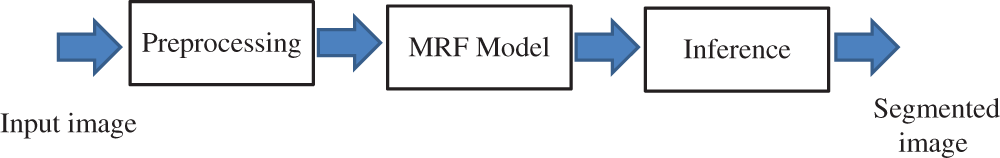
Figure 1: Overview of the proposed model
The parameters of the model are updated by using the Expectation Maximization (EM) algorithm. The algorithm does not takes into account the spatial information of pixels. This is because the data is assumed to be independent and identically distributed. The gap was addressed by considering Maximum a Posteriori (MAP) approach and by integrating the Markov Random Field (MRF) model into the framework. The proposed SVFMM manages to have a prior distribution for the set of parameters  which make use of Gibbs function as shown in Eq. (3) for incorporating a spatial description of pixels.
Primarily, the Gibbs function as described according to Eq. (3) facilitates in making probabilistic calculations about a pixel’s label for its relationship with a specific cluster. Fig. 2 taken from [11] illustrates the idea of pixel labels representing distinct clusters of image.


where 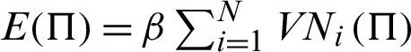 ,
,  represents regularization parameter whereas, Z serves as partition function and is described according to the Eq. (4). For pixel label vectors
  ,
,  describes the clique potential by looking into the neighborhood characterized by Ni where ‘i’ represents the i
 pixel. The Ni was described with the help of Eq. (5).

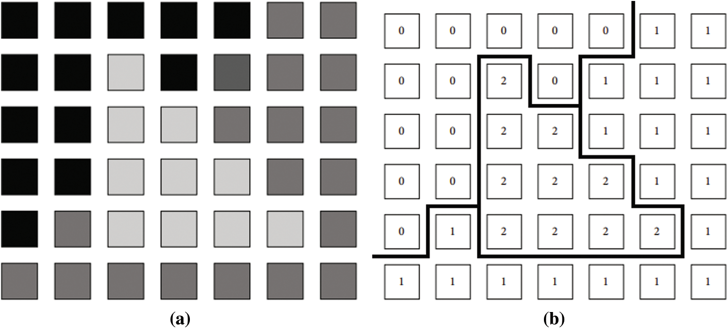
Figure 2: Example of pixel labels. (a) An image, (b) A labeling
How Gibbs Distribution Ensures Spatial Continuity?
According to [12], a digital image is defined by the finite rectangular grid of size M  N. Formally, it can be described according to Eq. (6).

Usually, these images consist of k number of finite classes. These classes are represented by  . The classification process, i.e.,
  aims to allocate a corresponding unique index from the user-defined class to each pixel in the image, i.e., Xij = qk where
  , which means that each pixel at
  belongs to class qk. If at location
  , the neighborhood of a pixel is denoted by
  then the following two conditions are taken into account.


Here Eq. (7) describes that a pixel cannot be a neighbor to itself whereas, Eq. (8) defines criteria for defining neighborhood of a specific pixel within the above mentioned 2D grid and additionally it represents a collection of subsets of L. With this understanding, the formal description of neighborhood system  of L can be given according to Eq. (9).

Neighborhood system has its roots in cliques. Formally, a clique C is a subset of the 2D grid, such that  . The set of clique C may consist of a single pixel or a group of pixels which are neighbors to each other under the influence of a specific neighborhood system. Therefore, for the pair
  the set of all such cliques is defined by Eq. (10). For image segmentation, a homogeneous neighborhood system plays an important role. This system can be described with the help Eq. (10).

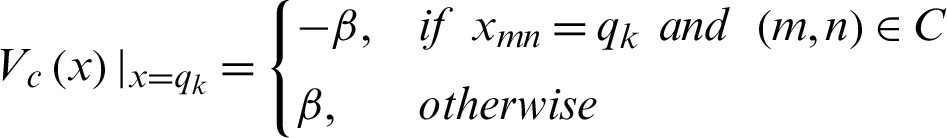
The values m, n, i, j, d and c are of type integer. Therefore, the first order neighborhood,  which takes into account the four nearest neighbors can be defined by putting c = 1. Similarly, the second-order neighborhood which considers eight nearest neighbors can be obtained by putting c = 2. The growing order of neighborhood supports the growth of corresponding clique types. However, generally, the first or second-order neighborhood system is employed. This configuration is found sufficient for ensuring spatial continuity among the image pixels. Each clique type holds a positive parameter. The clique potential for one point clique is described by

The two-point clique is defined as
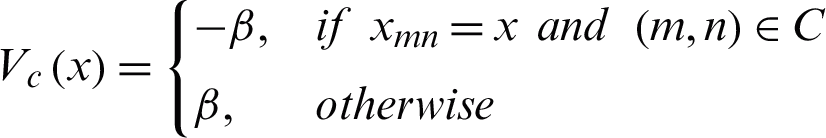
Both  ,
,  are positive constants and x is the index of the input image class to be determined for the pixel being considered and may take any value from Q. For making a practical decision, the entire set of probabilities for a pixel belonging to each class is computed and from this set a maximum probability is picked up for associating a specific pixel with a specific class.

where

Z represents normalization, constant T is a temperature parameter and  is a potential function.
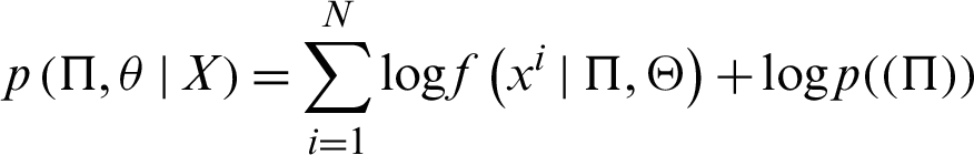
At this stage, by observing the events and the given model, there is a need to have the probability that can describe the unknown model parameter. For obtaining this description, a posterior probability is computed by using Eq. (13).

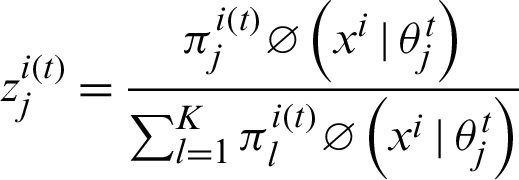
The unknown parameters of the mixture model are estimated by using the EM algorithm. The algorithm consists of E-step and M-step. The values of hidden variables are computed at E-step according to the Eq. (14).

The expected values according to SVFMM are maximized by using M-Step as described by Eq. (15). This step primarily aims to compute the log-likelihood function and provides a complete dataset.

where  , t describes the iteration step. The parameter of the model, i.e., the mean and the variance
  are updated according to Eqs. (16) and (17)


Though QMAP with respect to label parameter  can be maximized but the model has certain limitations. It is primarily unable to provide a closed-form of update equations. Secondly, the maximization procedure was supposed to work under the influence of certain constraints, i.e.,
  1 and
1 and  . To overcome this difficulty, SVFMM makes use of the Gradient Projection Algorithm for finding the label parameters which maximizes QMAP function [13]. The authors in [13] and [14] further improved the maximization step by differentiating Eq. (15) with respect to
  , and equating the result to zero reached to Eq. (18) [14].
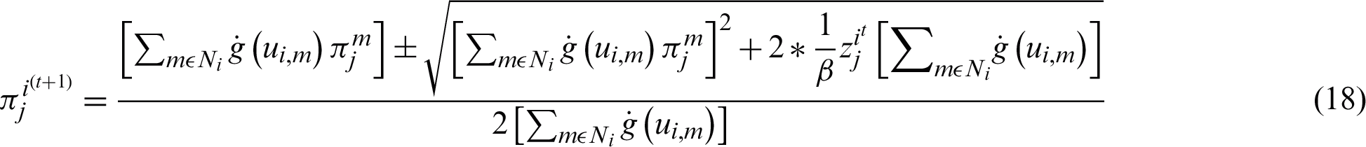
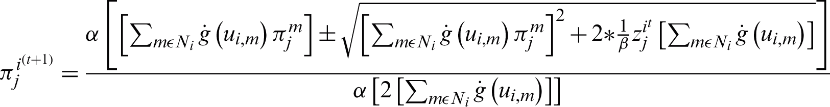
According to [15], the segmentation results are inconsistent if the value of the regularization parameter is close to 0, but with the value more than or equal to 2, the results are consistent. Therefore, the second half of the Eq. (18) suggests that the part of the equation 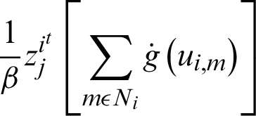 is twice as big as that of the part proposed in SCMM. This is a significant difference which notably impacted the segmentation results. The accuracy level was raised by using a weight factor with the new M-step. This weight factor was included according to the multiplicative property of equality. According to this property, suppose that if v = w, then
  , which implies that
  . For segmenting T1-Weighted simulated brain MR Images, this weighting factor, through trial and error method was 0.25. Therefore, the proposed weighted maximization step can be given according to the Eq. (19).
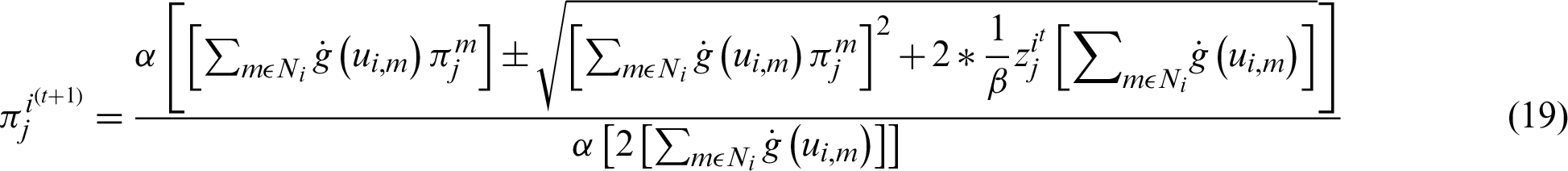
The above-shown maximization step was used in WSCFMM. This model outperformed the conventional SCMM and ensured reliability both in terms of time and precision.
The algorithm used in this study consists of the following steps [16].
Put  and initialize
 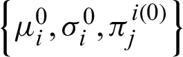 mean-variance and initial mixing probability.
The latent variable  is computed at E-step with the help of Eq. (14).
3.3 M-Step: Re-Estimation of Model Parameters 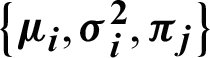


3.3.3 Updating Mixing Probabilities Eq. (19)
3.3.4 Evaluating Posterior Probability Eq. (13)
Here, convergence for parameter values and log-likelihood function is investigated. If the observed error is not less than 0.0001, then return to step 2 and set  .
.
The proposed model was used for segmenting T1-Weighted simulated brain MRIs. These MRIs are the specimen of complex multispectral images and can be downloaded from [17]. These images contain different levels of noise and different levels of intensity non-uniformity (INU). The noise levels vary from 0% to 9% comprising of only odd levels, whereas, the INU level varies from 0% to 40% with an increment of 20% respectively. For making different possible combinations of data, one factor was kept constant and the other was gradually varied. For example, by keeping the noise at 0%, INU was varied from 0% to 20% and then to 40%. This arrangement provided three images. Subsequently, the noise level was raised to 1% and INU level was again varied from 0% to 20% and then to 40%. This step provided another set of three images. The process was repeated for all levels of noise and all levels of INU. Eventually, a dataset with six different combinations of T1-Weighted normal brain MRIs was collected. Afterwards, this dataset was segmented through both models, i.e., SCMM and WSCFMM, one by one. To investigate the preciseness in the segmented images, ROIs from these segmented images were extracted. The Dice [18] and Jaccard [19] similarity measuring methods were used to compute the degree of similarity between the extracted ROI and GT segment. A higher degree of similarity indicates a higher level of accuracy and a lower degree of similarity indicates a lower level of accuracy.
Both the models, i.e., SCMM and WSCFMM were used to segment the test data. The results produced by both the models were analyzed from three different angles including the visual inspection of the results, the similarity between segmented ROI and the corresponding GT segment. The GT is obtained from the image with 0% noise and 0% INU.
The visual comparison between the results produced by both the models showed that WSCFMM was able to control the outliers and gave an appreciative level of performance in ideal conditions and in conditions where the candidate image is affected from intensity INU and/or noise.
Figs. 3 and 4 show the performance of WSCMM in comparison to SCMM. The results shown in the figures were obtained from the images affected with a higher level of noise, i.e., 7% and 9%, combined with different levels of INU. The visual investigations of these results show that besides outliers, SCMM is also unable to provide a well-defined segment. The circled region in Figs. 3 and 4 provides important observations which led us to the conclusion that a substantial portion of the information is missing. However, at the same settings of noise and INU, WSCFMM not only controlled the outliers but it also captured that missing information.
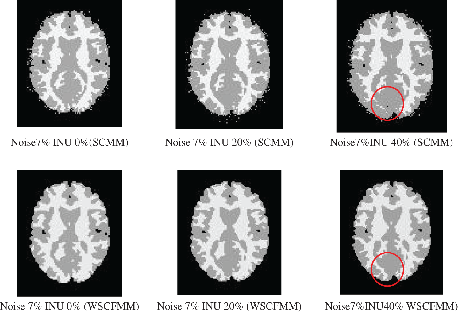
Figure 3: Visual comparison of images with 7% noise and INU varying from 0% to 40% segmented by SCMM and WSCFMM
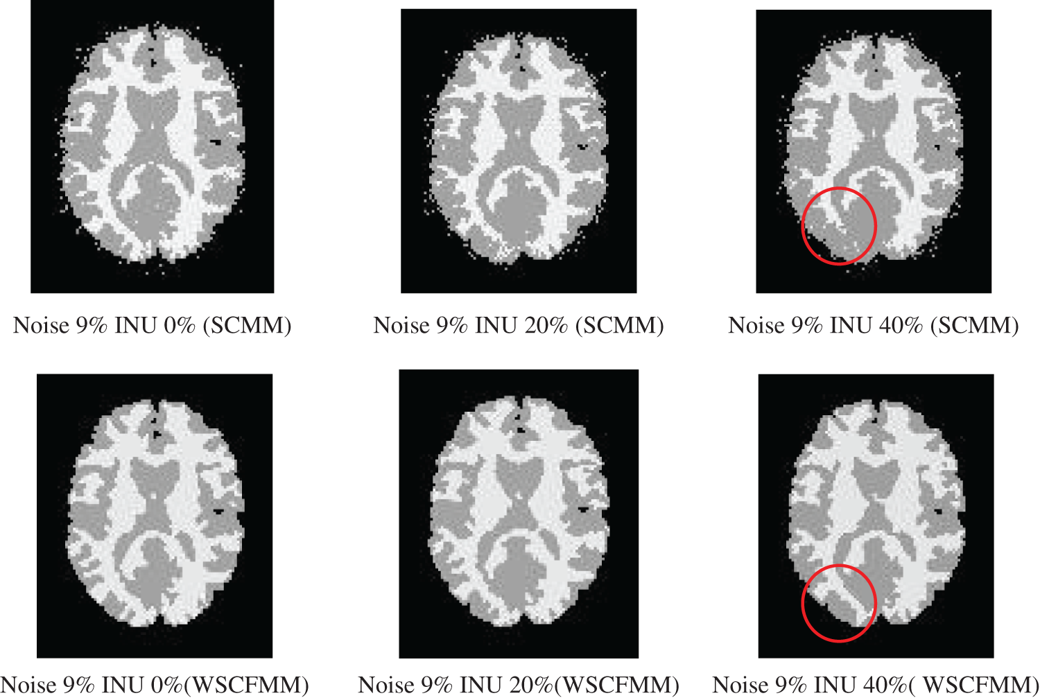
Figure 4: Visual comparison of images with 9% noise and INU varying from 0% to 40% segmented by SCMM and WSCFMM
5.2 Computational Comparison with Ground Truth Segment
An ROI was extracted by using both the models one by one. The extracted ROI by each model was compared with the GT. The degree of similarity of this extracted ROI was found by using Jaccard and Dice similarity measuring methods. These methods can be described with the help of the Eqs. (22) and (23).


The stability of the proposed model was investigated by considering all the available levels of noise and INU. The arrangement of test data used for completing this critical analysis is shown in Tab. 1. These tables provide a detailed description of the results obtained by using SCMM and WSCFMM. Both of these tables present and compare the mutual performance of the models on the individual slices. The percentage of accuracy of each slice with three different levels of INU was calculated by using Eq. (24).

Table 1: Similarity and average similarity of ROIs segmented by SCMM and WSFMM
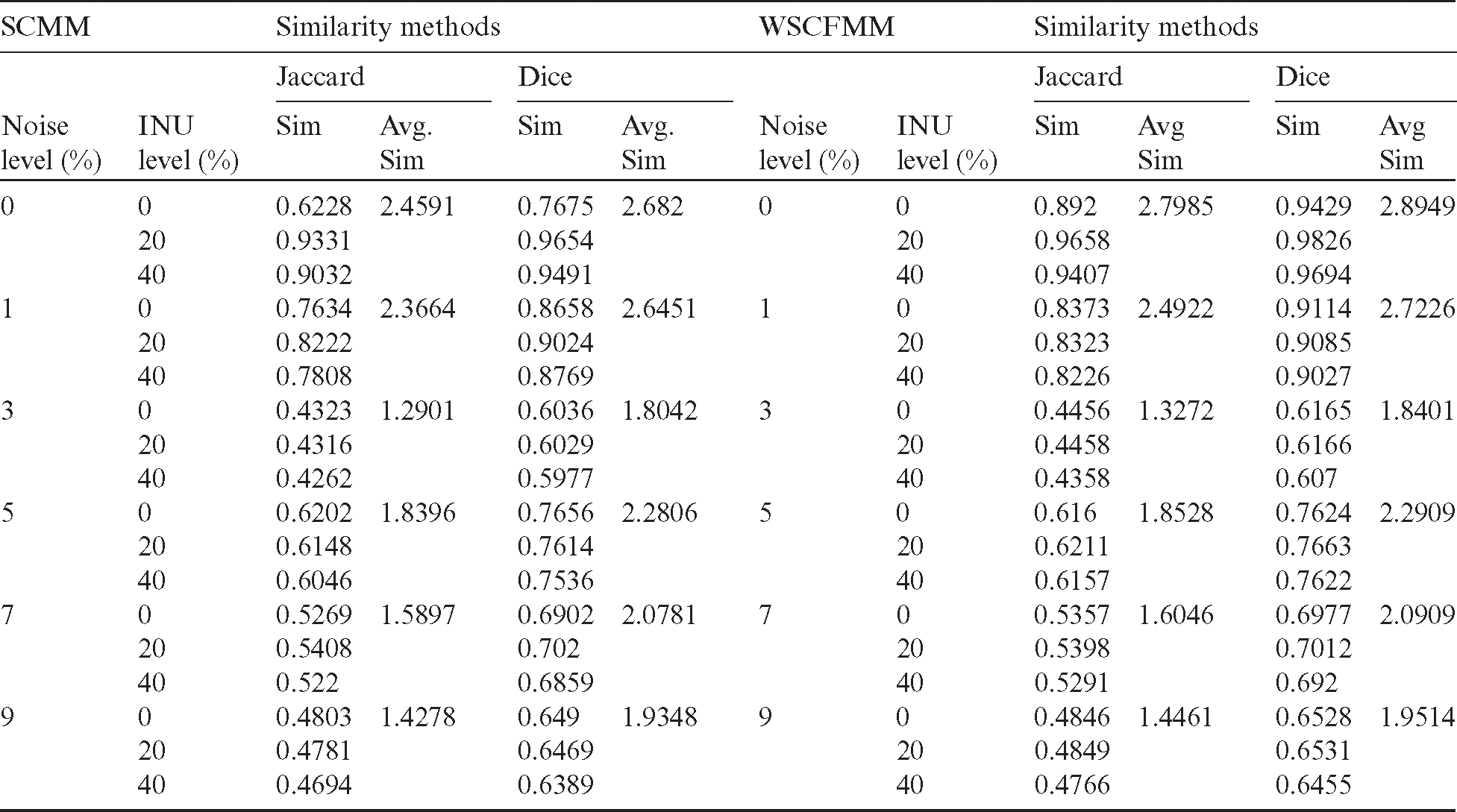
Results presented in Tab. 1 confirmed that WSCFMM outperformed SCMM in the noisy and noise-free environment. It can be observed that the performance of WSCFMM is appreciative either in a situation where there is no noise and/or in a situation where there is a mild noise. When the accuracy of the results was observed slice by slice, it was found that the Jaccard gave a higher average accuracy as compared to the Dice similarity measuring method, as shown in Fig. 5.
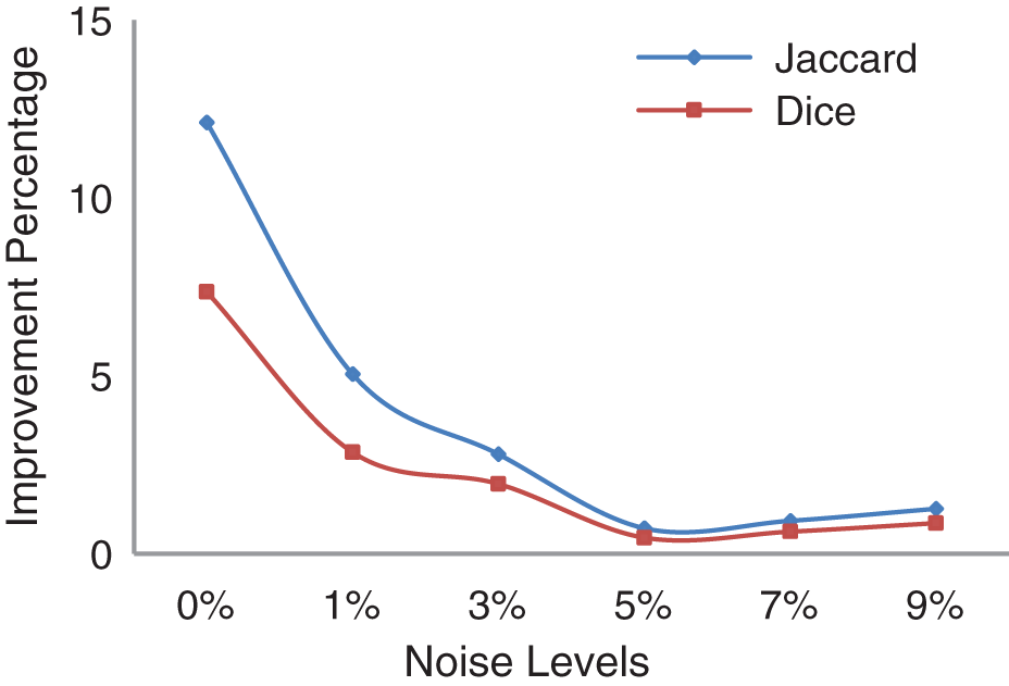
Figure 5: Average improvement achieved by WSCFMM
Similarly, to see an overall contribution of WSCFMM, an overall average accuracy of both the models was computed. This computation highlighted the significance of WSCFMM. It confirmed that according to the Jaccard similarity measuring method, WSCFMM has contributed an overall improvement of 4.76%, whereas, according to the Dice similarity measuring method, WSCFMM introduced an overall improvement of 2.65%, as shown in Fig. 6. This is a substantial improvement and it is expected to significantly affect the segmentation accuracy during the process of MRI analysis.
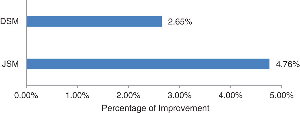
Figure 6: Overall average accuracy of WSCFMM according to the dice similarity method (DSM) and jaccard similarity method (JSM)
During MRI’s examination, ‘time’ is a critical issue. As chances for the accumulation of a large MRI dataset for a single subject cannot be completely ruled out, so it is highly desirable to work with a model that has a predictable nature. WSCFMM is one such model that uses a small amount of processing time without compromising the accuracy.
The case of SCMM is weak in terms of its processing time. It utilizes a variable amount of time for processing the same dataset under similar experimental conditions. By introducing the derivational fixture and by adding a weight factor, WSCFMM has efficiently controlled the issue of variable execution time. Besides, it has stabilized the model and has significantly enhanced the segmentation accuracy.
The mutual comparison of SCMM and WSCFMM for the processing time is presented in Fig. 7. The results were obtained by considering all levels of noise, i.e., from 0–9%, and all level of INU, i.e., from 0–40%.
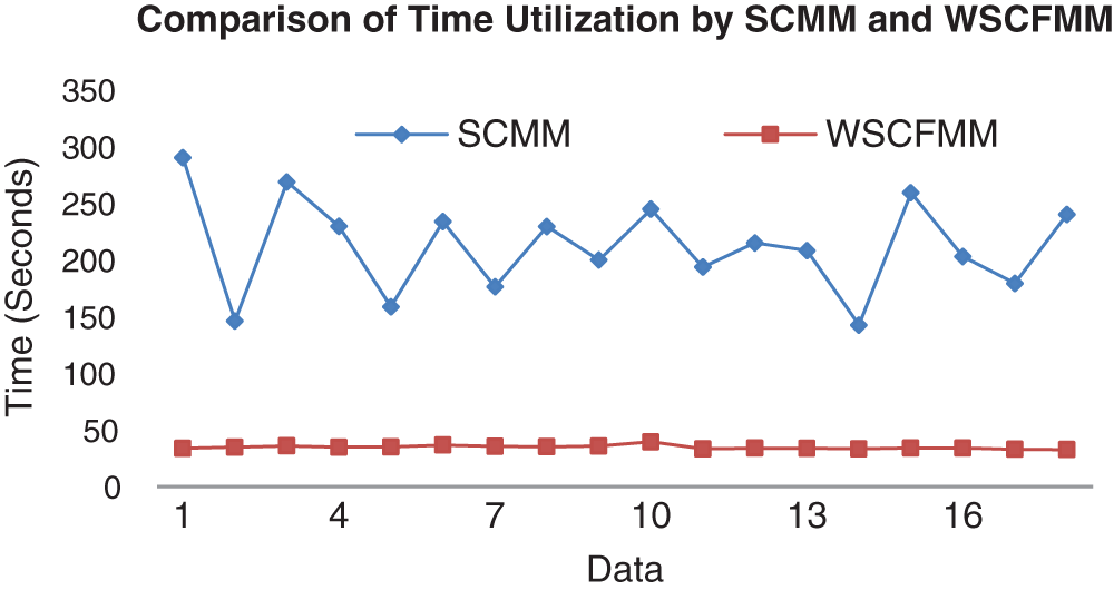
Figure 7: Mutual comparison of the execution time
According to the results presented in Fig. 7, WSCFMM has displayed a predictable behavior by utilizing the approximately constant amount of processing time for each image. Whereas, SCMM processes the same data by using a different amount of time.
Fig. 8 presents the mutual comparison of the average performance of both the models for segmenting every single combination of data. As mentioned earlier, this dataset consists of six different combinations. Every single combination, which in turn consists of three different images, is represented by one anchor point. Fig. 8 shows a mutual comparison of the average time used by both the models for segmenting every single combination of data. In terms of efficiency, it has depicted a marked improvement of WSCFMM over the SCMM.
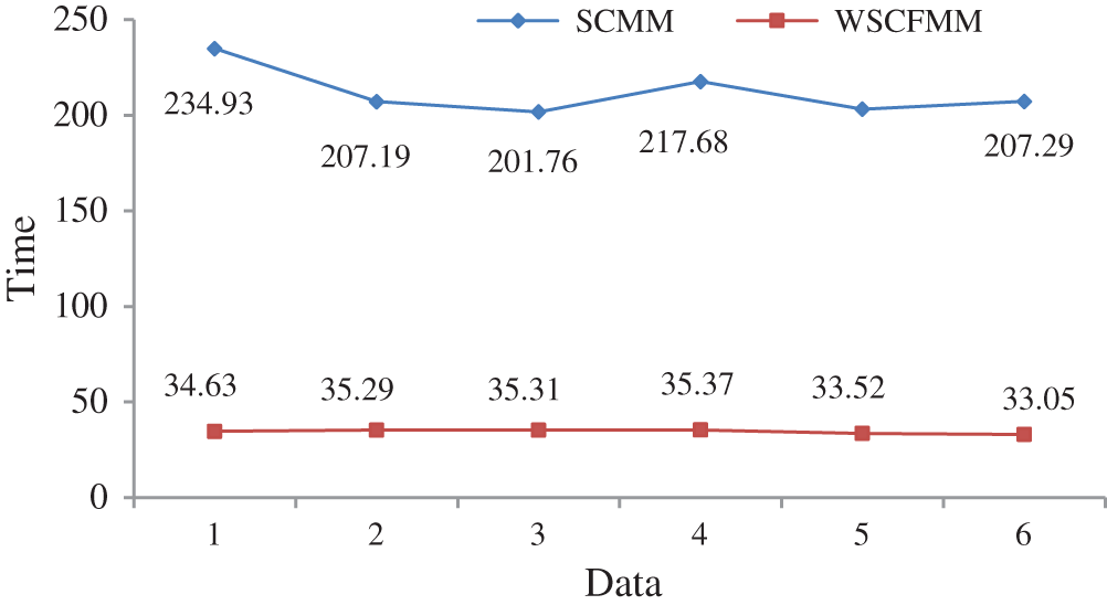
Figure 8: Mutual comparison of the average execution time utilized by both the models
The overall contribution of WSCFMM in terms of processing time utilization is presented in Fig. 9. The WSCFMM not only made the model predictable and reliable but was also instrumental in bringing down the execution time from 1272.04 s to 207.17 s. This leads to WSCFMM’s achievement of 83.71% improvement. This is an encouraging improvement and broadens the chances for comfortably handling large MRI datasets.
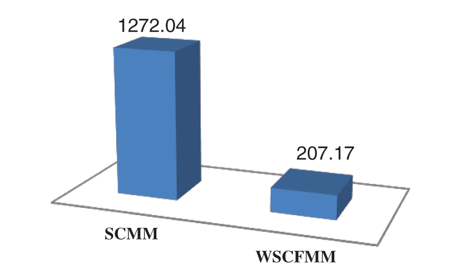
Figure 9: Cumulative average execution time utilized by both the models
The segmentation results produced by the WSCFMM enjoy an excellent superiority when compared to the segmentation results produced by the SCMM. The comparison made over the basis of human visual system undoubtedly confirmed that the WSCFMM has displayed an appreciative level of stability and has produced convincing results even under abnormal conditions, i.e., in the presence of various levels of noise and INU. The strength of the proposed WSCFMM was judged by finding the similarity of the segmented ROI with the GT. For that matter, Dice similarity and Jaccard similarity measuring methods were used. Both of these methods supported the claim that WSCFMM is a stable, reliable and efficient method. According to the Jaccard similarity measuring method, the proposed model has shown an overall improvement of 4.76%, and according to the Dice similarity measuring method, it has shown an overall improvement of 2.65%. Moreover, the proposed WSCFMM was found to be exceptionally efficient as it reliably brought down the processing time from 1272.04 s to 207.17 s. This leads to an overall efficiency of 83.71%. The proposed WSCFMM would be beneficial for the field of medical imaging, mainly due to its ability to maintain consistency and reliability in the segmentation procedures. It is expected to be highly desirable by the experts especially working in the areas of brain imaging as any loss of the relevant details or inaccurate results can be extremely fatal for the patients under treatment.
Funding Statement: The author(s) received no specific funding for this study.
Conflicts of Interest: The authors declare that they have no conflicts of interest to report regarding the present study.
References
1. H. Li, C. Pan, Z. Chen, A. Wulamu and A. Yang. (2020). “Ore image segmentation method based on U-Net and watershed,” Coumputers, Materials & Continua, vol. 65, no. 1, pp. 563–578.
2. J. Hu, Z. Lei, X. Li, Y. He and J. Zhou. (2020). “Ultrasound speckle reduction based on histogram curve matching and region growing,” Computers, Materials & Continua, vol. 65, no. 1, pp. 705–722.
3. L. Li, L. Sun, J. Guo, S. Li and P. Jiang. (2020). “Identification of crop diseases based on improved genetic algorithm and extreme learning machine,” Computers, Materials & Continua, vol. 65, no. 1, pp. 761–775.
4. J. Niu, Y. Jiang, Y. Fu, T. Zhang and N. Masini. (2020). “Image deblurring of video surveillance system in rainy environment,” Computers, Materials & Continua, vol. 65, no. 1, pp. 807–816.
5. L. Geng, C. Cui, Q. Guo, S. Niu, G. Zhang. (2020). et al., “Robust core tensor dictionary learning with modified Gaussian mixture model for multispectral image restoration,” Computers, Materials & Continua, vol. 65, no. 1, pp. 913–928.
6. J. Vacher, P. Mamassian and R. Coen-Cagli. (2018). “Probabilistic model of visual segmentation,” arXiv preprint arXiv: 1806. 00111.
7. A. Wadhwa, A. Bhardwaj and V. Singh Verma. (2019). “A review on brain tumor segmentation of MRI images,” Magnetic Resonance Imaging, vol. 61, pp. 247–259.
8. J. Vacher and R. Coen-Cagli. (2019). “Combining mixture models with linear mixing updates: Multilayer image segmentation and synthesis,” arXiv preprint arXiv: 1905.10629.
9. T. Xiong, L. Zhang and Z. Yi. (2016). “Double Gaussian mixture model for image segmentation with spatial relationships,” Journal of Visual Communication and Image Representation, vol. 34, pp. 135–145.
10. A. Gómez-Villa, G. Díez-Valencia1 and A. E. Salazar-Jimenez. (2016). “A Markov random field image segmentation model for lizard spots,” Revista Facultad de Ingeniería, Universidad de Antioquia, vol. 79, pp. 41–49. [Google Scholar]
11. T. Liu, X. Huang and J. Ma. (2016). “Conditional random fields for image labeling,” Mathematical Problems in Engineering, vol. 2016, no. 6, pp. 1–15. [Google Scholar]
12. D. Zhang, L. J. Van Gool and A. Oosterlinck. (1994). “Classification of remote sensing images with the aid of Gibbs distribution,” Image and Signal Processing for Remote Sensing, vol. 2315, pp. 462–472. [Google Scholar]
13. K. Blekas, A. Likas, N. P. Galatsanos and I. E. Lagaris. (2005). “A spatially constrained mixture model for image segmentation,” IEEE Transactions on Neural Network, vol. 16, no. 2, pp. 494–498. [Google Scholar]
14. C. Nikou, N. P. Galatsanos and A. C. Likas. (2007). “A class-adaptive spatially variant mixture model for image segmentation,” IEEE Transactions on Image Processing, vol. 16, no. 4, pp. 1121–1130. [Google Scholar]
15. Z. Kato and T. C. Pong. (2006). “A Markov random field image segmentation model for color textured images,” Image and Vision Computing, vol. 24, no. 10, pp. 1103–1114. [Google Scholar]
16. N. Iriawan, A. A. Pravitasari, K. Fithriasari Irhamah, S. W. Purnami and W. Ferriastuti. (2019). “Mixture model for image segmentation using Gaussian, Student’st, and Laplacian distribution with spatial dependence,” in The 2nd Int. Conf. on Science, Mathematics, Environment and Education, vol. 2194, no. 1, pp. 20042. [Google Scholar]
17. [Online]. Available http://www.bic.mni.mcgill.ca/brainweb. [Google Scholar]
18. S. Klein, U. A. Van der Heide, I. M. Lips, M. Van Vulpen, M. Staring. (2008). et al., “Automatic segmentation of the prostate in 3D MR images by atlas matching using localized mutual information,” Medical Physics, vol. 35, no. 4, pp. 1407–1417. [Google Scholar]
19. M. Murugavel and J. M. Sullivan Jr. (2009). “Automatic cropping of MRI rat brain volumes using pulse coupled neural networks,” Neuroimage, vol. 45, no. 3, pp. 845–854. [Google Scholar]
 | This work is licensed under a Creative Commons Attribution 4.0 International License, which permits unrestricted use, distribution, and reproduction in any medium, provided the original work is properly cited. |

