DOI:10.32604/cmc.2021.014620
| Computers, Materials & Continua DOI:10.32604/cmc.2021.014620 | |
| Article |
Power Inverted Topp–Leone Distribution in Acceptance Sampling Plans
1Faculty of Science, Umm AL-Qura University, Makkah Al Mukarramah, 715, Saudi Arabia
2Faculty of Graduate Studies for Statistical Research, Cairo University, Giza, 12613, Egypt
3Obour High Institute for Management & Information, Al-Sharqua, 44516, Egypt
4Faculty of Business Administration, Sinai University, Al-Arish, 45511, Egypt
*Corresponding Author: Said G. Nassr. Emails: dr.saidstat@gmail.com; said.gamal@su.edu.eg
Received: 03 October 2020; Accepted: 21 November 2020
Abstract: We introduce a new two-parameter model related to the inverted Topp–Leone distribution called the power inverted Topp–Leone (PITL) distribution. Major properties of the PITL distribution are stated; including; quantile measures, moments, moment generating function, probability weighted moments, Bonferroni and Lorenz curve, stochastic ordering, incomplete moments, residual life function, and entropy measure. Acceptance sampling plans are developed for the PITL distribution, when the life test is truncated at a pre-specified time. The truncation time is assumed to be the median lifetime of the PITL distribution with pre-specified factors. The minimum sample size necessary to ensure the specified life test is obtained under a given consumer’s risk. Numerical results for given consumer’s risk, parameters of the PITL distribution and the truncation time are obtained. The estimation of the model parameters is argued using maximum likelihood, least squares, weighted least squares, maximum product of spacing and Bayesian methods. A simulation study is confirmed to evaluate and compare the behavior of different estimates. Two real data applications are afforded in order to examine the flexibility of the proposed model compared with some others distributions. The results show that the power inverted Topp–Leone distribution is the best according to the model selection criteria than other competitive models.
Keywords: Inverted Topp–Leone distribution; acceptance sampling plans; maximum likelihood estimators; weighted least squares estimators; Bayesian estimators
The inverted (inverse) distributions have considerable applications in several area including; biological sciences, life testing problems, survey sampling, engineering sciences, etc. Many inverted distributions and their applications have been devoted by several authors; for instance, Keller et al. [1] studied the shapes of the density and failure rate functions for the inverse Weibull model. Reference [2] proposed a generalized inverse Weibull distribution with decreasing and unimodal failure rates. Reference [3] proposed the inverse Lindley distribution and studied its main properties. The inverted Kumaraswamy distribution has been discussed in [4]. The inverted Nadarajah–Haghighi distribution with decreasing and upside-down bathtub hazard rate was discussed in [5]. Reference [6] proposed and studied the inverse power Lomax distribution. Reference [7] introduced inverted exponentiated Lomax distribution and estimated the distribution for right censored data. Reference [8] introduced the inverted Topp–Leone (ITL) distribution and discussed several properties.
The cumulative distribution function (CDF) of random variable Y has the ITL distribution with shape parameter  is defined by:

The probability density function (PDF) related to (1) is given by

In recent times, several extended and generalized formulations of the classical distributions, based on different procedures, have been discussed by several authors (see for example [9–13]). The power transformation (PT) approach is one of the most important methods that have been employed for this purpose. It is employed to create new distributions out of the well-known distributions through adding an additional parameter. This approach allows more flexible model able to describe different types of real data. PT procedure for several distributions has been provided by several researches (see, for example [14–16]).
Acceptance sampling (AS) concerns with inspection and decision-making regarding lots of product and constitutes one of the oldest techniques in quality assurance. A typical application of AS is as follows:
Required: A company receives a shipment of product from a vendor. This product is often a component or raw material used in the company’s manufacturing process.
1. Sampling: A sample is taken from the lot and the relevant quality characteristic of the units in the sample is inspected.
2. Decision: On the basis of the information of the given sample, a decision is made regarding lot disposition to accept or to reject the lot.
3. For AS: Accepted lots are put into production,
For rejected samples: Rejected lots may be returned to the vendor or may be subjected to some other lot disposition action.
The objective of this research is to provide a generalized formula of the ITL model by employing the PT as  , where Y has the ITL distribution. We call the modified form of ITL model as the PITL distribution. The PITL model is able to (i) give favorite properties owing to the additional shape parameter; (ii) give more flexibility of the PDF and hazard rate function (HRF); (iii) provide more flexibility of the kurtosis compared to ITL model; (iv) develop a sampling plan, derive its operating characteristic function and give the corresponding decision; (v) estimate the model parameters based on different methods of estimation, and (vi) analyze two read data.
This paper involves the following sections. In Section 2, we introduce the two-parameter PITL distribution. Section 3 gives some stractural properties of the PITL distribution. The design of proposed AS plan under a truncated life test is discussed in Section 4. Section 5 discusses parameter estimation of the PITL model based on the maximum likelihood (ML), maximum product of spacing (MPS), least squares (LS), weighted LS (WLS) and Bayesian methods. Section 6 provides a numerical study. Real data are analyzed in Section 7 and the article finishes with concluding remarks.
2 Power Inverted Topp–Leone Distribution
In this section, we define a new probability distribution related to the ITL distribution via a PT method. The formulae of its PDF, CDF, survival function (SF), HRF and cumulative HRF are given.
Definition:
A random variable X is said to have the PITL distribution if we employ the PT  , where Y has the ITL distribution with CDF(1). The CDF of a random variable has the PITL distribution with shape parameters
  and
and  , denoted by
 , is defined by

The PDF of the PITL distribution related to (3) is given by:

For,  , the PDF (4) provides the ITL distribution (see [8]). The survival function;
  , and the HRF;
 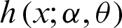 of the PITL distribution are, respectively, given by

and

Plots of the PDF and HRF are presented in Fig. 1 for some choice’s values of parameters.
Figure 1: The PDF and HRF plots for the PITL distribution
The shape of the PITL PDF could be inverted bathtub, reversed J-shape, unimodal, and positively skewed. The shape of the HRF of the PITL shows that it is increasing, decreasing, reversed J-shape and up-side down.
This section gives some necessary characteristics of the PITL distribution such as; the probability weighted moments, the kth moment, the moment-generating function (MGF), inequality measures, rth moment of the residual lifetime (RL), Rényi entropy, and stochastic ordering.
3.1 Probability Weighted Moments
The probability weighted moments (PWM) are ordinarily used to find estimators of the parameters and quantiles of distributions. The PWM of X (for  ,
,  ) is defined by:

Use binomial expansion for  as follows:

The PWM of the PITL distribution is obtained by substituting PDF (4) and CDF (8) in (7) as follows:

Employ the following generalized binomial expansion, where b > 0 is real non integer and  ,
,

in  then we get

where 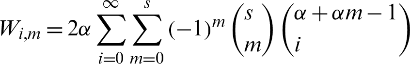 and
and  is the gamma function.
Here, we present the kth moment, MGF, and quantile analysis of the PITL  distribution. The kth moment for the PITL is derived as follows:

The first four moments about zero are obtained after putting k = 1, 2, 3, 4 in (12). The MGF of the PITL distribution is given by

The kth central moment ( ) of the PITL distribution is given by:

Moreover, we obtain quantile function of the PITL, say 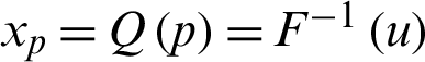 , by inverting (3) as follows:
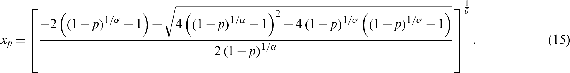
In particular, the first three quartiles, say Q1, Q2 and Q3 are obtained by setting u = 0.25, 0.5, 0.75 respectively, in (15).
The Bonferroni curve (BC) as well as Lorenz curve (LC) are widely useful not only in economics to study income and poverty, but also in other fields, such as reliability, insurance and medicine. The LC and BC of the PITL model are derived, respectively, as follows:
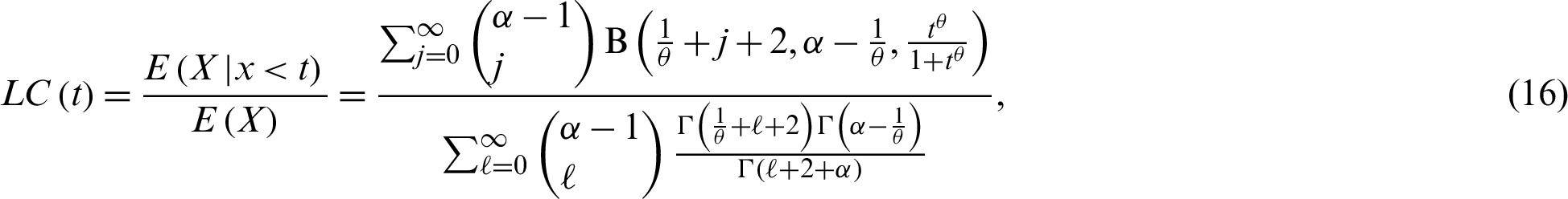
and
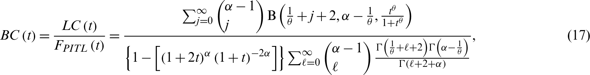
where  is the incomplete beta function.
3.4 Residual and Reversed Residual Life Functions
Here we obtain the rth moment of the RL of the PITL model. The rth moment of RL is defined as follows

The rth moment of the RL of the PITL distribution is derived by using the binomial expansion and the PDF (4) in (18), as follows:

An important application of the moments of RL is the mean which represents the expected additional life length for an item which is working at age t and obtained by putting r = 1 in (19).
On contrast, the reversed RL is defined as the conditional random variable  which denotes the time elapsed from the failure of a component given that its life is less than or equal to t. The rth moment of the reversed RL for PITL distribution is given by

The mean of reversed RL serves as the waiting time elapsed since the failure of an item on condition that this failure had occurred.
The entropy of a random variable is a measure of the uncertainty variation. The Rényi entropy of PITL distribution is obtained as follows:
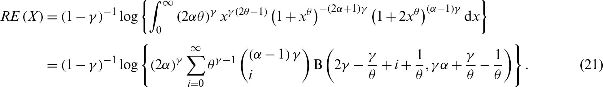
The  -entropy is defined by

Therefore, the  -entropy of the PITL distribution is given by

Let X and Y are independent random variables with CDFs Fx and Fy respectively, X is said to be smaller than Y if the following ordering holds (see [17]):
• Stochastic order ( ) if
) if  for x.
• Likelihood ratio order ( ) if
) if  is decreasing in x.
• Hazard rate order ( ) if
) if  for all x.
• Mean residual life order ( ) if
) if  for all x.
We have the following chain of implications among the various partial orderings mentioned above:
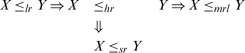
To show that the random variable X is smaller than Y, where X and Y have the PITL with different parameters, so we prove the above conditions, mentioned in [17], in the following theorem
Theorem 1: Let X  PITL
PITL  and
and  PITL
PITL  . If
. If  and
and  , then
  ,
,  ,
,  , and
, and  .
.
Proof
It is sufficient to show  is a decreasing function of x; the likelihood ratio is

Therefore,
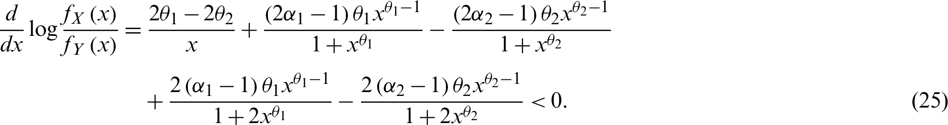
Thus,  is decreasing in x and hence
  . Similarly, we can conclude that for
  .
.
We assume that the lifetime of a product follows the PITL distribution with parameters ( ) defined by (4) and the specified median lifetime of the units claimed by a producer is m0. Our interest is to make an inference about the acceptance or rejection of the proposed lot based on the criterion that the actual median lifetime, m, of the units is larger than the prescribed lifetime m0. A common practice in life testing is to terminate the life test by a pre-determined time t0 and note the number of failures. Now to observe median lifetime, the experiment is run for a t0 = am0 units of time, multiple of claimed median lifetime with any positive constant a. The idea to accept the proposed lot based on the evidence that
  , given probability of at least p*(consumer’s risk) using single acceptance sampling plan is as follows [18].
Draw a random sample of n number of units from the proposed lot and conduct an experiment for t0 units of time. If during the experiment c or less number of units (acceptance number) fail then accept the whole lot, other than the lot is rejected. Observe that probability of accepting a lot, consider sufficiently large sized lots so that the binomial distribution can be applied, under the proposed sampling plan is given by

where  defined by (3). The function L(p) is the operating characteristic function of the sampling plan, i.e., the acceptance probability of the lot as function of the failure probability. Further using t0 = am0, thus p0 can be written as

Now, the problem is to determine for given values of  and c the smallest positive integer n such that

where p0 is given by (27).
By solving the inequality in (28) for n with given consumer’s risk p*, positive constant a, acceptance number c and p0, which computed according to parameters  and t0. The solution of the inequality in (28) depends on searching the minimum value of n which makes the left-hand side of the given inequality is less than or equal 1 − p*.
The minimum values of n satisfying the inequality (28) and its corresponding operating characteristic probability are obtained and displayed in Tabs. 1–3 for the following assumed parameters:
1.  , c = 0(2)8.
2.  (Note that when a = 1,
  ).
).
3.  .
.
Table 1: Single sampling plan for PITL distribution at 
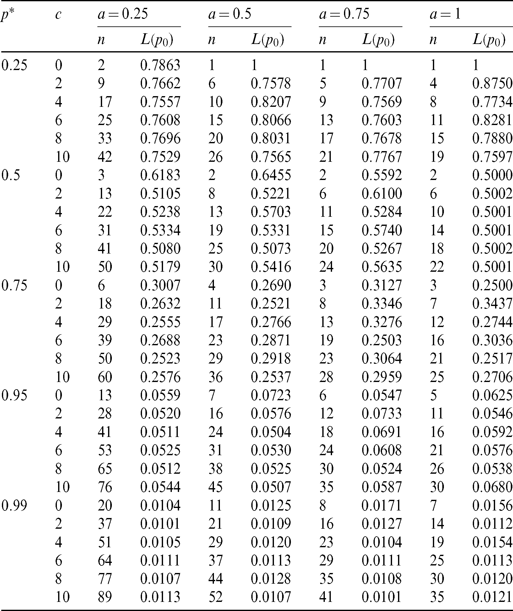
Table 2: Single sampling plan for PITL distribution at  ,
, 
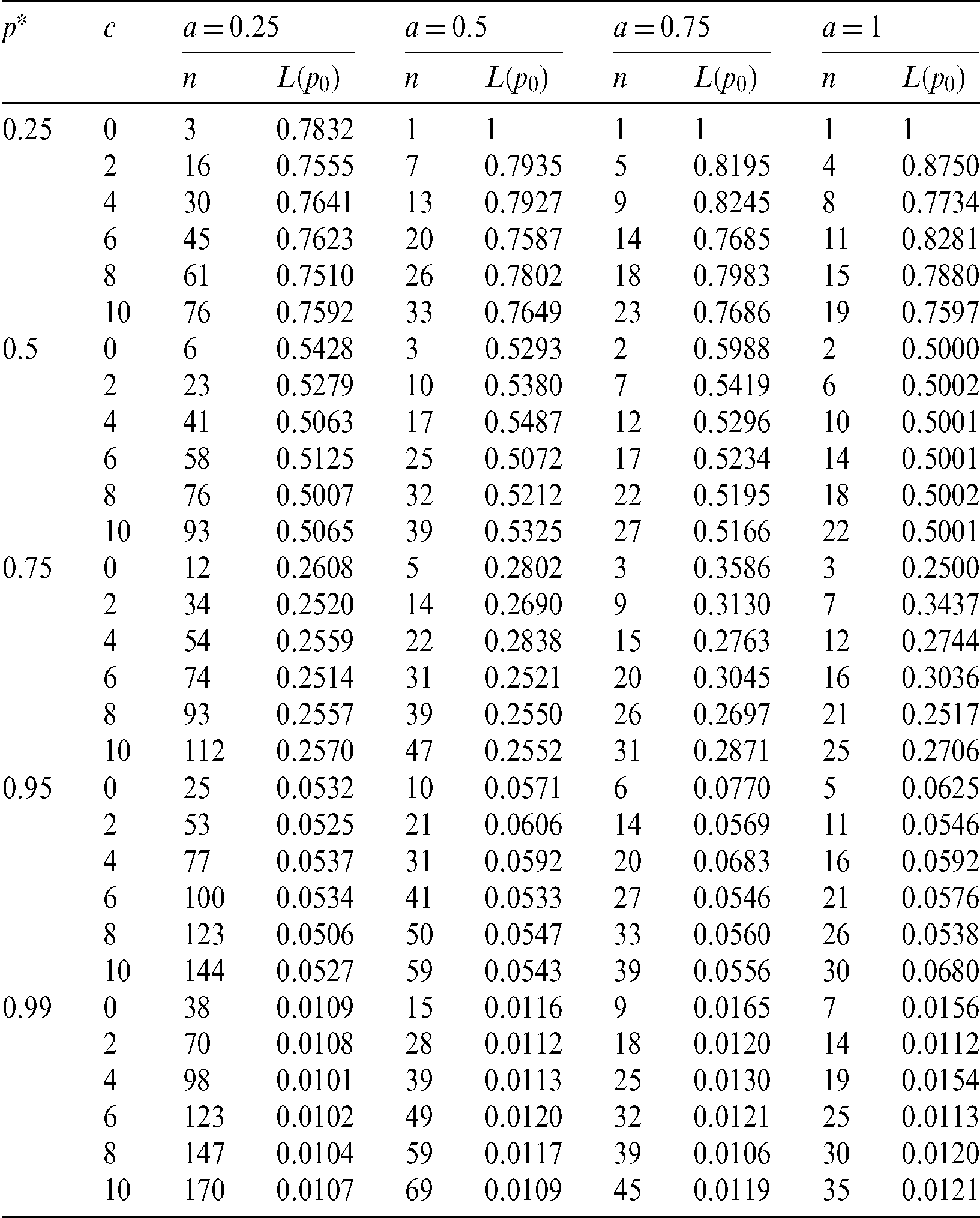
Table 3: Single sampling plan for PITL distribution at  ,
, 
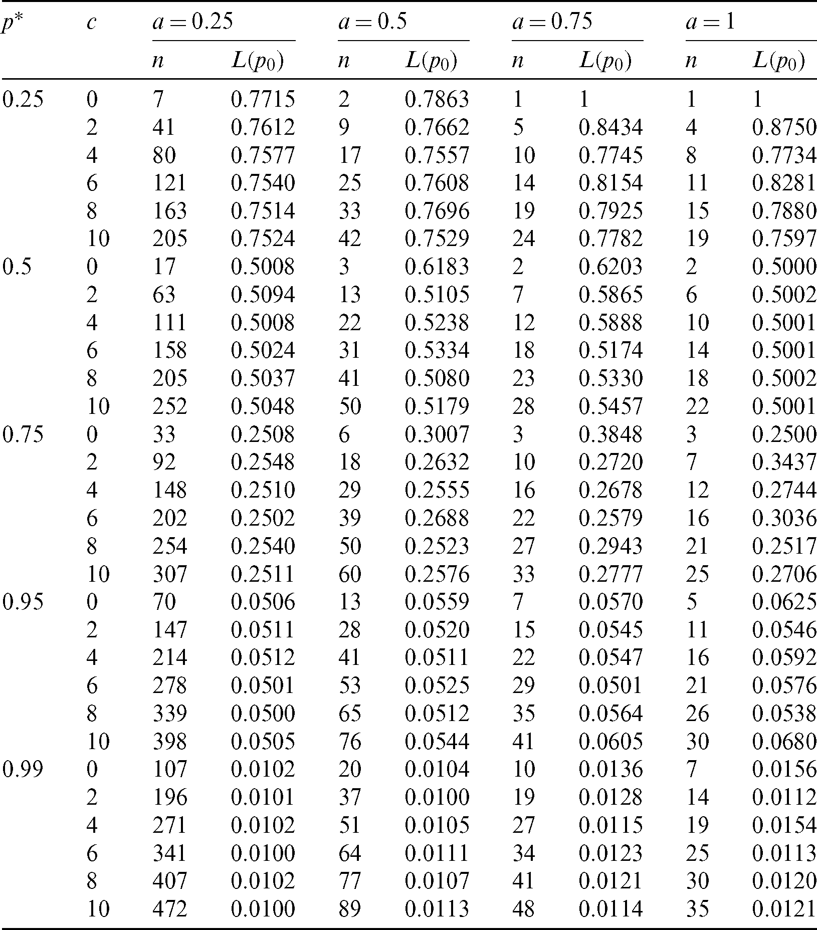
From the results obtained in Tabs. 1–3, we notice that:
• With increasing p*, the required sample size n is increasing.
• With increasing c, the required sample size n is increasing.
• With increasing a, the required sample size n is decreasing.
• With increasing  and fixed
  , the required sample size n is increasing.
• With increasing  , and fixed
  , the required sample size n is increasing.
Finally, for all results checked that  . Also, when a = 1, we have p0 = 0.5, as t0 = m0 and hence all results (n, L(p0)) for any vector of parameter
  are the same.
In this section, the parameter estimation of the PITL distribution is discussed using classical and Bayesian estimation methods. The classical methods include ML, MPS, LS, and WLS.
Let  be the observed random sample from the PITL distribution with PDF (4). The log-likelihood function of the PITL distribution, denoted by
  , for parameters, based on complete sample, is given by

The partial derivatives of  with respect to
  and
and  are given by

and,

The non-linear equations  and
and  are solved numerically via iterative technique, to get the ML estimators of
  and
and  .
.
A strong alternative procedure, known as MPS, for estimating the population parameters of continuous distributions was proposed in [19]. Let

be the uniform spacings of a random sample from the PITL distribution, where

The MPS estimator is obtained by maximizing the geometric mean (GM) of the spacings

with respect to  and
and  , or we maximize the logarithm of the GM of sample spacings (34) with respect to
  and
and  . The numerical technique is used to otain the desired estimators.
5.3 Least Squares and Weighted Least Squares Estimators
Let  is a random sample of size n drawn from the PITL distribution and let
  be the observed ordered sample. The LS estimators are derived by minimizing the sum of squares errors,

related to the population parameters. So, the LS estimators of the model parameters of the PITL distribution are obtained by minimizing the following formula
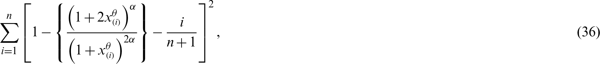
related to  and
and  . Furthermore, the WLS estimators of the PITL distribution is obtained by minimizing the following related to
  and
and  .
.
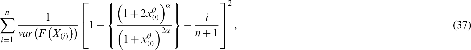
where,  .
.
The Bayesian estimator using squared error loss function (SELF) under the assumption of non-informative prior of the population parameters for PITL distribution is obtained. Assuming the prior distributions of  and
and  have uniform density function, where the joint prior PDF are given by

The posterior density of  and
and  given the data is

Therefore, the Bayesian estimators of  under SELF; denoted by
  can be calculated as follows:

Generally, the ratio of two integrals given by (40) cannot be obtained in a closed form. Then, the integral Eq. (40) is solved numerically due to its complicated forms.
As mentioned in previous section, expressions for the derived estimators are hard to obtain. Therefore, we design simulation study for clarifying the theoretical results. The behavior of estimates is examined in terms of their mean square error (MSE), and relative bias (RB). We perform the following:
Step 1: 10000 random samples of sizes 20, 50, 75 and 150 are generated from PITL distribution. The chosen parameters values are;
 ,
,  ,
,  ,
,  ,
,  ,
,  ,
,  ,
,  .
.
Step 2: ML estimate (MLE), MPS estimate (MPSE), LS estimate (LSE), WLS estimate (WLSE) and Bayes estimate (BE) of the parameters are obtained.
Step 3: Markov Chain Monte Carlo (MCMC) technique (as M-H algorithm) is used to get the BEs of  and
and  under SELF via 10000 iterations.
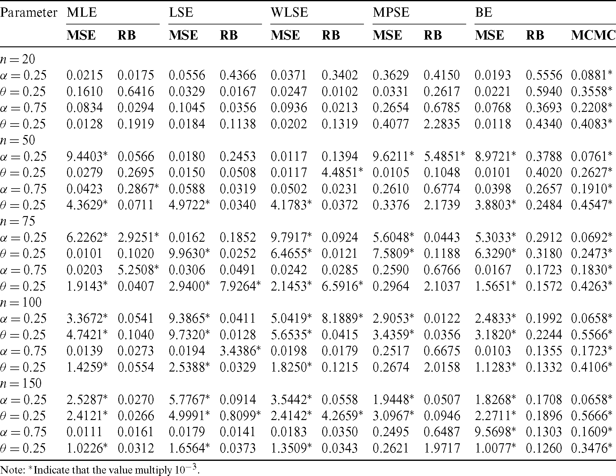
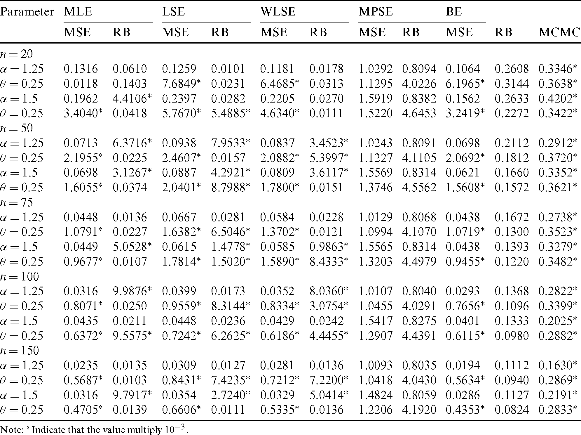
Step 4: Compute MSEs and RBs of all estimates and the results are listed in Tabs. 4–7. We notice the following about the performance of estimates:
• For all methods of estimation, it is clear that MSEs and RBs decrease as n gets larger for all parameters (see Tabs. 4–7).
• The MSEs of BS are the less than the corresponding for other methods in almost all cases (see Tabs. 4–7).
• For fixed value of  and as the value of
  gets larger, the MSEs and RBs of
  estimates are increasing for different methods (see Tabs. 4–7).
• For fixed value of  and as the value of
  decreases, the MSEs and RBs of
  estimates are decreasing for different methods (see Tabs. 4–7).
• For fixed value of  and as the value of
  increases, the MSEs and RBs of
  estimates increase based on the different methods. But the MSEs and RBs of estimates of
  decrease for different methods (see Tabs. 4–7).
• For fixed value of  and as the value of
  decreases, the MSEs and RBs of
  estimates decrease based on the different methods. While the MSEs and RBs of
  estimates for different methods increase (see Tabs. 4–7).
Table 4: The MSE, RB and MCMC for different estimates of the PITL distribution
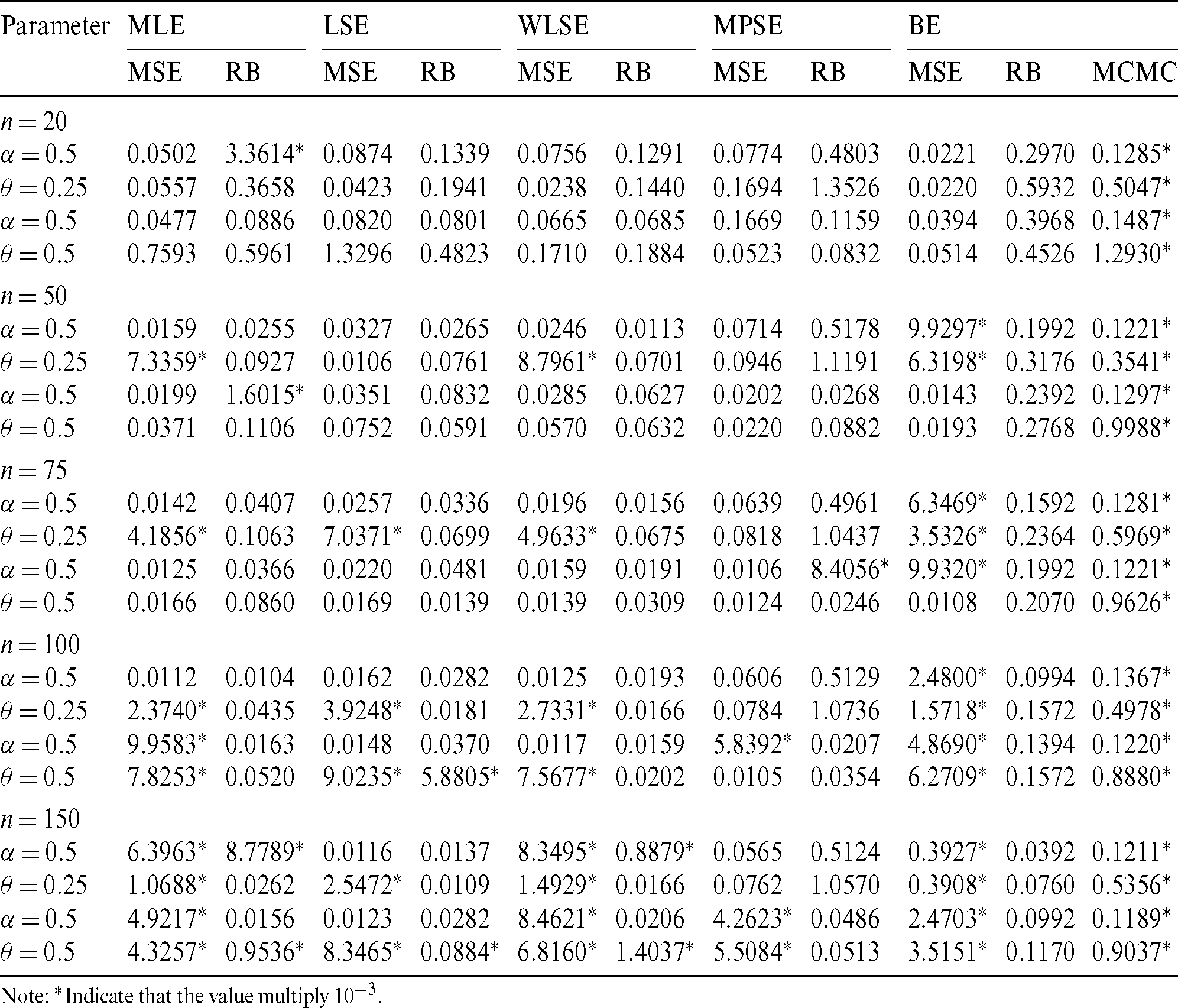
Note: *Indicate that the value multiply 10−3.
Table 5: The MSE, RB and MCMC for different estimates of the PITL distribution
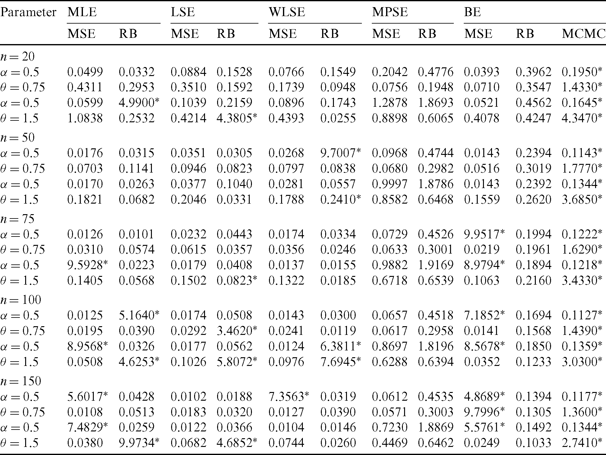
Table 6: The MSE, RB and MCMC for different estimates of the PITL distribution
Note: *Indicate that the value multiply 10−3.
Table 7: The MSE, RB and MCMC for different estimates of the PITL distribution
Note: *Indicate that the value multiply 10−3.
This section gives applications of the PITL model using two real data sets. The fits of the PITL distribution, for the first data, is compared with Type II Topp–Leone inverse Rayleigh (TIITLIR) [20], inverse Weibull (IW), exponentiated generalized power function (EGPF) [21], power function (PF), and the inverse exponential (IE) distributions. On the other hand, the fits of the PITL distribution, for the second data, is compared with TIITLIR, IW, Kumaraswamy Weibull Lomax (KWL) [22], inverse Rayleigh (IR) and Lomax (L) distributions. Criteria is handled to inspect the distribution for best fit: Akaike information criteria (AIC), consistent AIC (CAIC), Bayesian information criteria (BIC), Hannan and Quinn information criteria (HQIC). Also, we provide the Kolmogorov Smirnov (KS) statistic and the P value. The engineering application of selecting and comparing different distributions in composite structures can be found in [23].
First Data: The data set contains 34 observations of the vinyl chloride data obtained from [24] which represents clean up gradient ground–water monitoring wells in mg/L. Tab. 8 gives measures of comparison for the various distributions under study. Also, it contains the MLE and the corresponding standard error (SE) for parameters of each model. Plots of estimated PDF and CDF are given in Fig. 3. The PP plots of estimated densities are given in Fig. 2.
Table 8: The MLEs and SEs of the model parameters and goodness of fit measures for first data
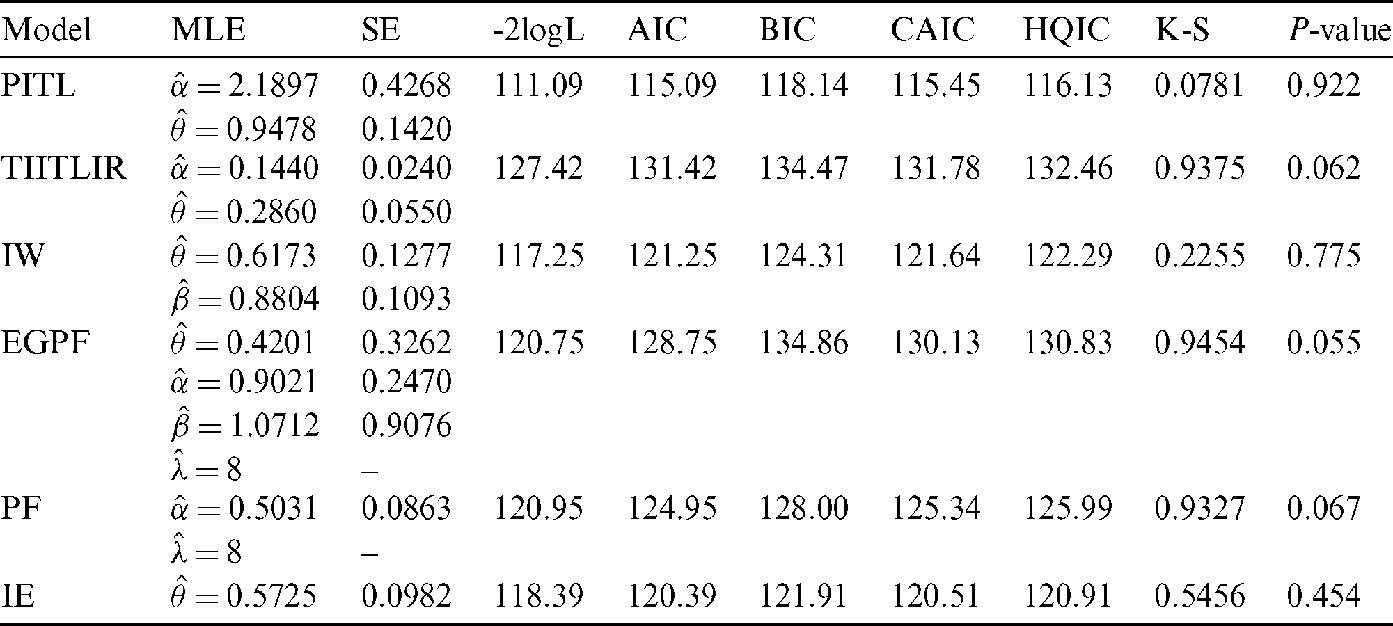
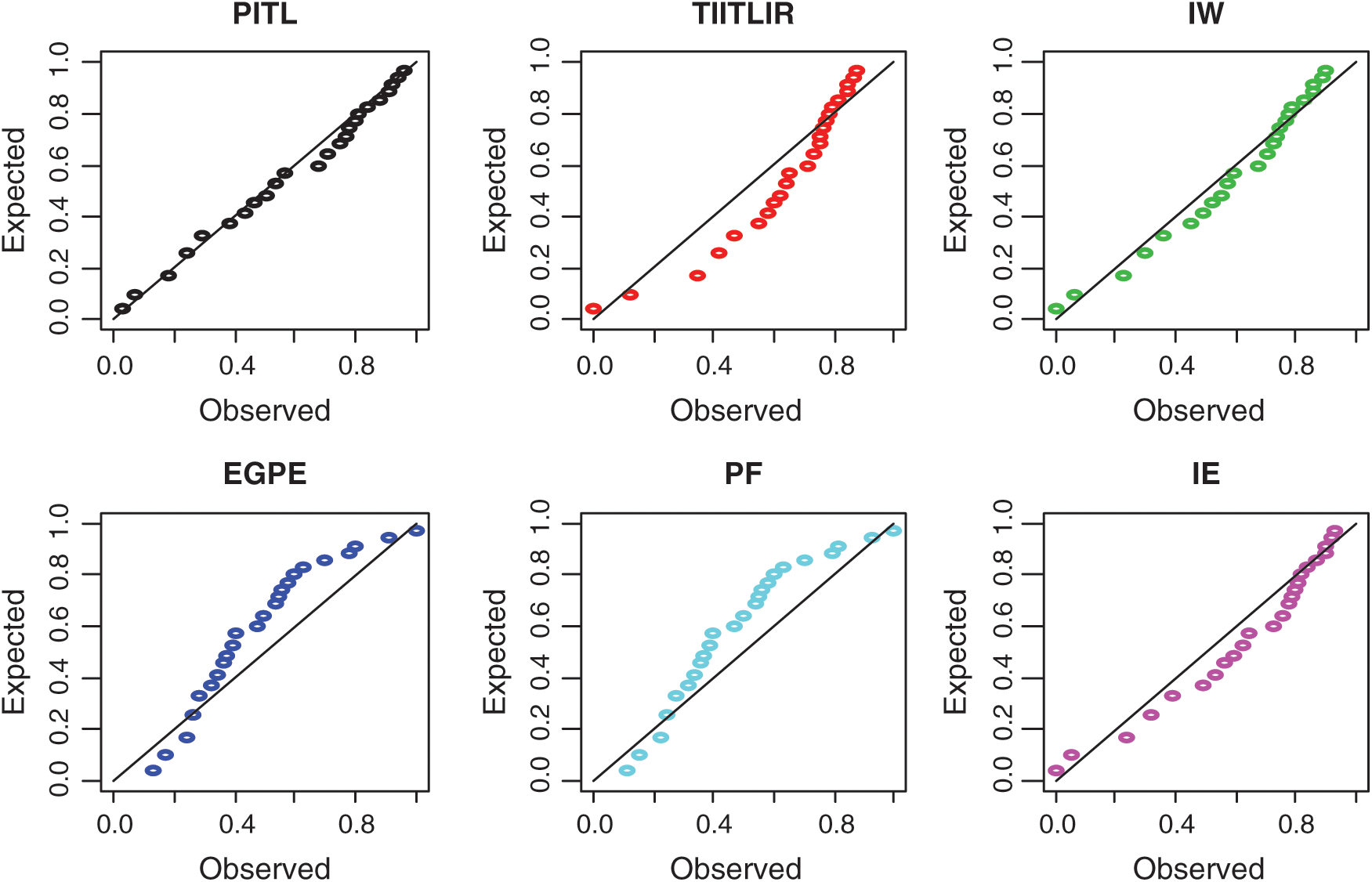
Figure 2: The PP plots of PITL, TIITLIR, IW, EGPF, PF and IE distributions for first data set
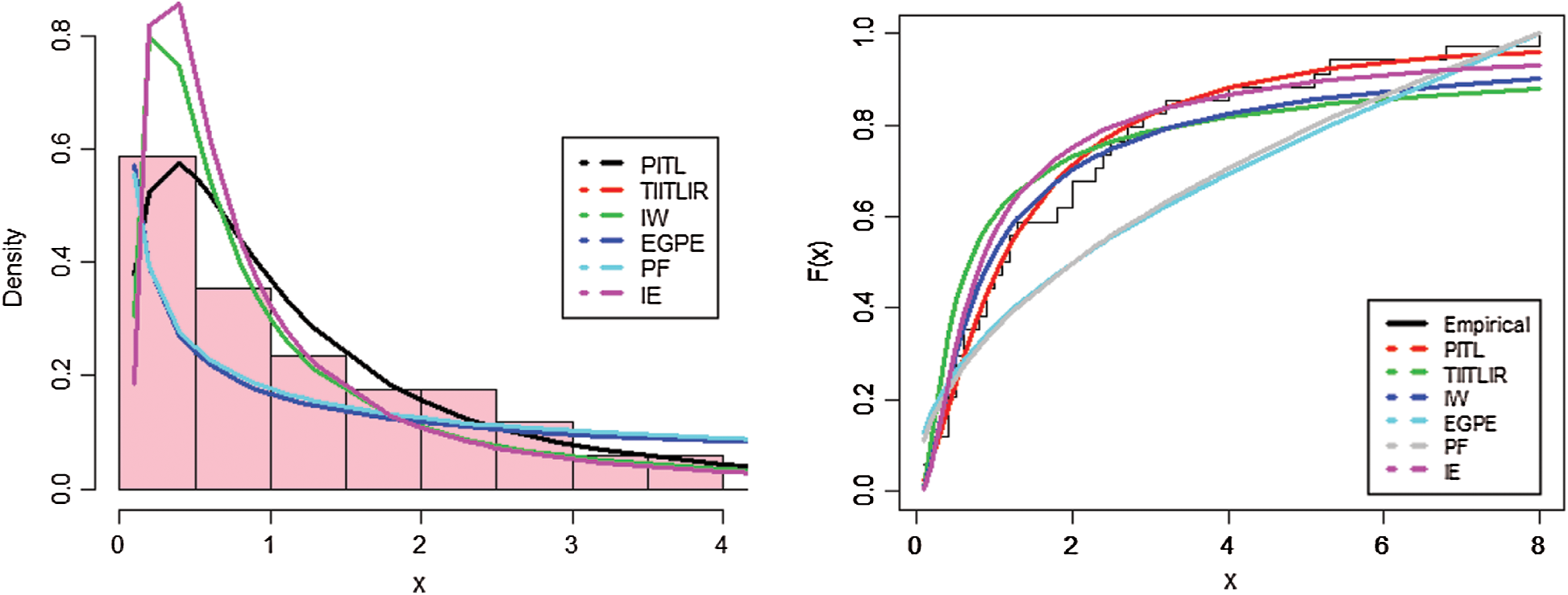
Figure 3: Estimated PDF and CDF of the models for the first data set
Second Data: The second real-life data was originally reported in [25]. The data contain 30 observations of the March precipitation (in inches) in Minneapolis/St Paul. The observed values are:
0.77, 1.74, 0.81, 1.20, 1.95, 1.2, 0.47, 1.43, 3.37, 2.2, 3, 3.09, 1.51, 2.1, 0.52, 1.62, 1.31, 0.32, 0.59, 0.81, 2.81, 1.87, 1.18, 1.35, 4.75, 2.48, 0.96, 1.89, 0.9, 2.05.
Tab. 9 provides comparison measures for the proposed distributions. Plots of estimated PDF and CDF of the PITL model are given in Fig. 4. PP plots of estimated densities are given in Fig. 5.
Table 9: The MLEs and SEs of the model parameters and goodness of fit measures for second data
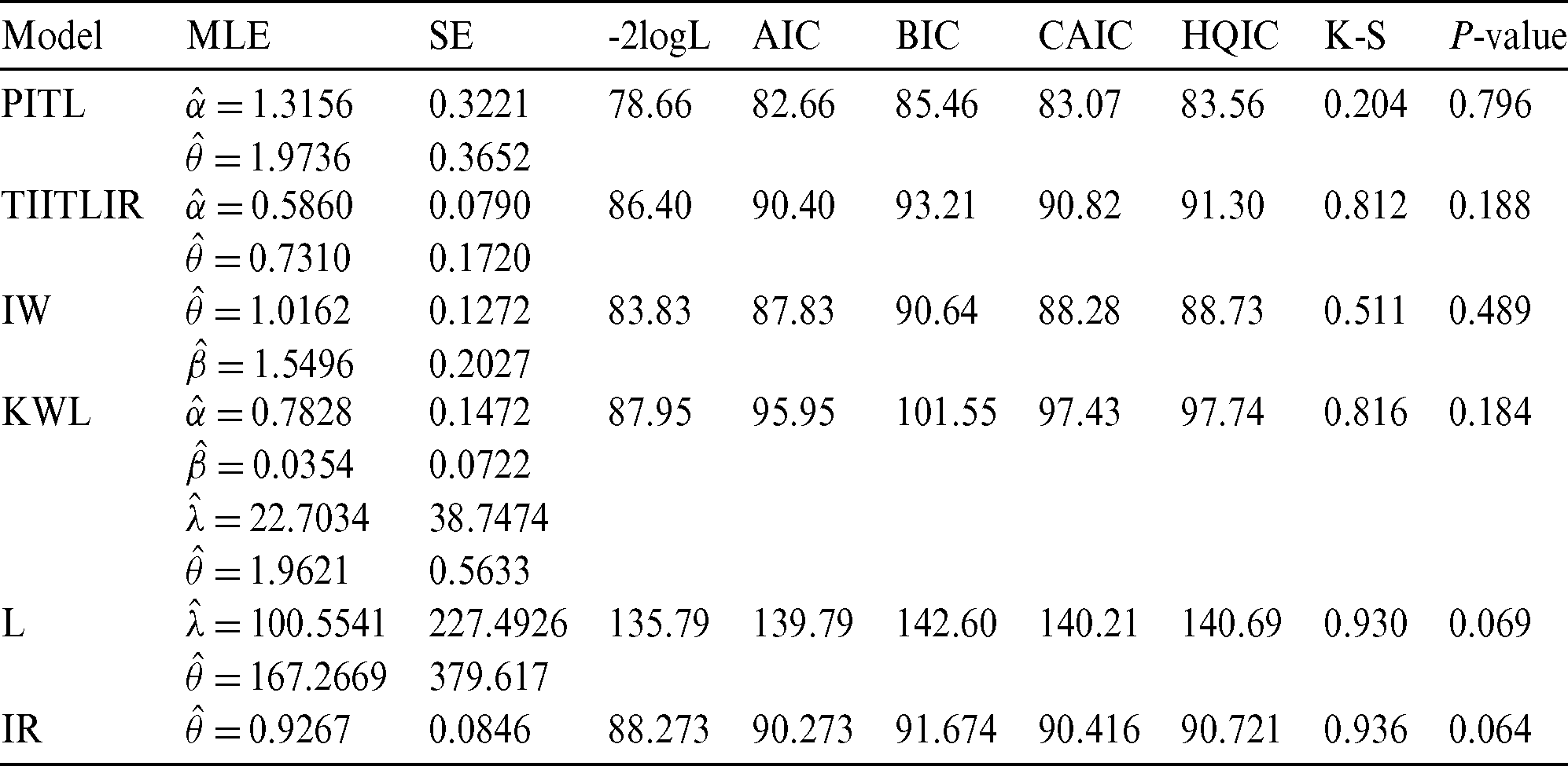
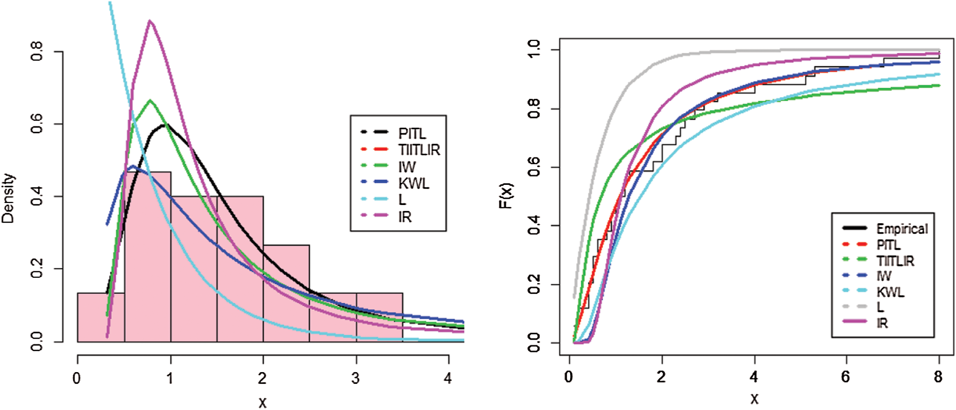
Figure 4: Estimated PDF and CDF of the models for the second data set
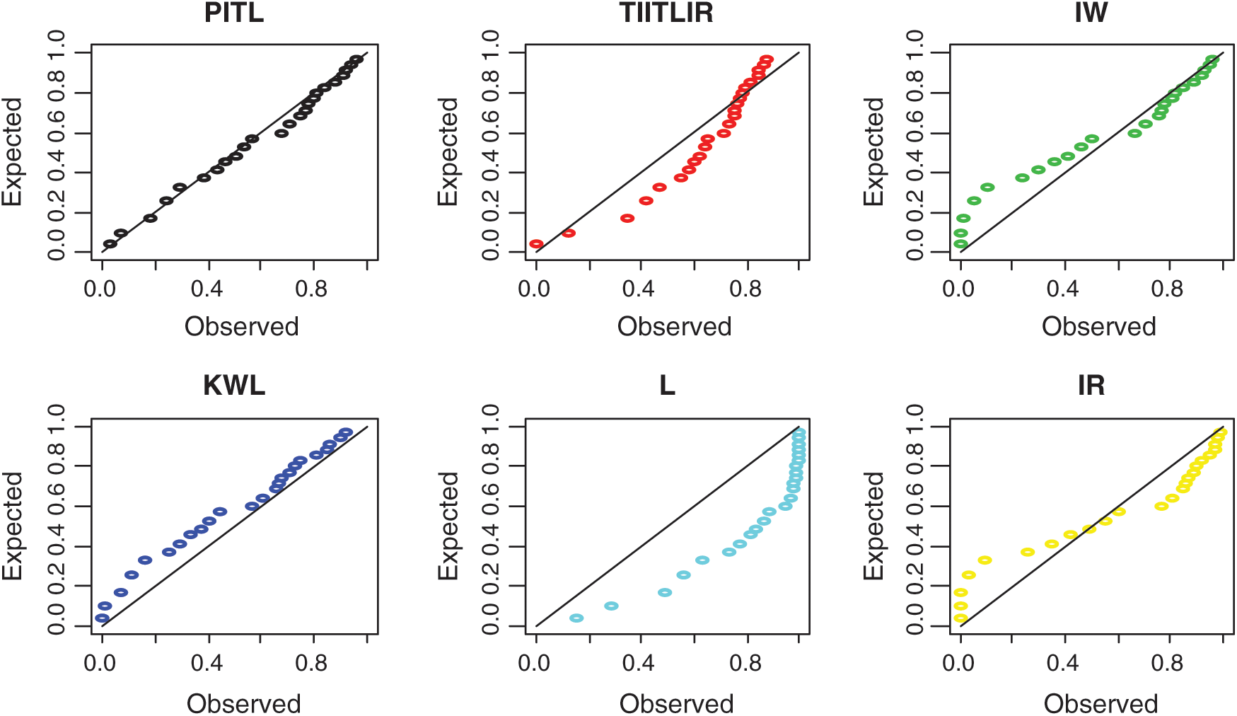
Figure 5: The PP plots of PITL, TIITLIR, IW, KWL, L and IR distributions for second data set
Based on Tabs. 8 and 9 and Figs. 2–5, it can be seen that the PITL provides the overall best fit. Consequently, the PITL distribution can be chosen as suitable model when comparing to other distributions to explain the studied data.
In this study, the power inverted Topp–Leone distribution is proposed. It provides more flexibility compared with the inverted Topp–Leone model. Some useful statistical properties of the PITL distribution are provided. We obtain the acceptance sampling plans for the PITL distribution when the life test is truncated at the median life of the stated distribution. At different parameters of the PITL distribution and different levels of consumer’s risk, the minimum sample size is computed under multiple truncation times. Also, at the obtained sample sizes, the probability of acceptance is computed to ensure that it’s less than or equal the complement of the consumer’s risk (1 − P*). The model parameters are estimated by the maximum likelihood, maximum product spacing, least squares, weighted least squares and Bayesian methods. A simulation study reveals that the estimates have desirable properties such as small relative biases and mean square errors as sample sizes increase. Then, we deal with two real data application and mention that the PITL model is the better than other competitive distributions.
Acknowledgement: The authors would like to thank the editor and the anonymous referees for their valuable and very constructive comments, which have greatly improved the contents of the paper.
Funding Statement: The author(s) received no specific funding for this study.
Conflicts of Interest: The authors declare that they have no conflicts of interest to report regarding the present study.
References
1. A. Z. Keller and A. R. R. Kamath. (1982). “Alternative reliability models for mechanical systems,” in Third Int. Conf. on Reliability and Maintainability, Toulse, France.
2. F. R. S. de Gusmão, E. M. M. Ortega and G. M. Cordeiro. (2011). “The generalized inverse Weibull distribution,” Statistical Papers, vol. 52, no. 3, pp. 591–619.
3. V. K. Sharma, S. K. Singh, U. Singh and V. Agiwal. (2015). “The inverse Lindley distribution: A stress-strength reliability model with application to head and neck cancer data,” Journal of Industrial and Production Engineering, vol. 32, no. 3, pp. 162–173.
4. A. M. Abd AL-Fattah, A. A. El-Helbawy and G. R. Al-Dayian. (2017). “Inverted Kumaraswamy distribution: Properties and estimation,” Pakistan Journal of Statistics, vol. 33, no. 1, pp. 37–61.
5. M. H. Tahir, G. M. Cordeiro, S. Ali, S. Dey and A. Manzoor. (2018). “The inverted Nadarajah–Haghighi distribution: Estimation methods and applications,” Journal of Statistical Computation and Simulation, vol. 88, no. 14, pp. 2775–2798.
6. A. S. Hassan and M. Abd-Allah. (2019). “On inverse power Lomax distribution,” Annals of Data Science, vol. 6, no. 2, pp. 259–278.
7. A. S. Hassan and R. E. Mohamed. (2019). “Parameter estimation for inverted exponentiated Lomax distribution with right censored data,” Gazi University Journal of Science, vol. 32, no. 4, pp. 1370–1386.
8. A. S. Hassan, M. Elgarhy and R. Ragab. (2020). “Statistical properties and estimation of inverted Topp–Leone distribution,” Journal of Statistics Applications & Probability, vol. 9, no. 2, pp. 319–331.
9. A. S. Hassan and S. G. Nassr. (2018). “Power Lomax Poisson distribution: Properties and estimation,” Journal of Data Science, vol. 18, pp. 105–128.
10. A. S. Hassan and S. G. Nassr. (2021). “Transmuted Topp–Leone power function: Theory and application,” Journal of Statistics Applications and Probability, vol. 10, no. 2, . [Online] Available: http://www.naturalspublishing.com/FC.asp?JorID=3. [Google Scholar]
11. A. S. Hassan, E. A. Elshrpieny and R. E. Mohamed. (2019). “Odd generalized exponential power function distribution: Properties and applications,” Gazi University Journal of Science, vol. 32, no. 1, pp. 351–370. [Google Scholar]
12. A. S. Hassan, M. Elgarhy, S. G. Nassr, Z. Ahmed and S. Alrajhi. (2019). “Truncated Weibull Frèchet distribution: Statistical inference and applications,” Journal of Computational and Theoretical Nanoscience, vol. 16, pp. 1–9. [Google Scholar]
13. A. S. Hassan, M. A. Sabry and A. M. Elsehetry. (2020). “Truncated power Lomax distribution with application to flood data,” Journal of Statistics Applications & Probability, vol. 9, no. 2, pp. 347–359. [Google Scholar]
14. M. E. Ghitany, D. K. Al-Mutairi, N. Balakrishnan and L. J. Al-Enezi. (2013). “Power Lindley distribution and associated inference,” Computational Statistics and Data Analysis, vol. 64, pp. 20–33. [Google Scholar]
15. E. H. A. Rady, W. A. Hassanein and T. A. Elhaddad. (2016). “The power Lomax distribution with an application to bladder cancer data,” SpringerPlus, vol. 5, no. 1, pp. 2144. [Google Scholar]
16. A. S. Hassan, S. M. Assar and A. M. Abd Elghaffar. (2020). “Statistical properties and estimation of power transmuted inverse Rayleigh distribution,” Statistics in Transition, New Series, vol. 21, no. 3, pp. 93–107. [Google Scholar]
17. M. Shaked and J. G. Shanthikumar. (2007). Stochastic Orders, New York: Springer. [Google Scholar]
18. S. Singh and Y. M. Tripathi. (2017). “Acceptance sampling plans for inverse Weibull distribution based on truncated life test,” Life Cycle Reliability and Safety Engineering, vol. 6, pp. 169–178. [Google Scholar]
19. R. C. H. Cheng and N. A. K. Amin. (1983). “Estimating parameters in continuous univariate distributions with a shifted origin,” Journal of the Royal Statistical Society: Series B (Methodological), vol. 45, no. 3, pp. 394–403. [Google Scholar]
20. H. F. Mohammed and N. Yahia. (2019). “On Type II Topp Leone inverse Rayleigh distribution,” Applied Mathematical Sciences, vol. 13, no. 13, pp. 607–615. [Google Scholar]
21. A. S. Hassan and S. G. Nassr. (2020). “A new generalization of power function distribution: Properties and estimation based on censored samples,” Thailand Statistician, vol. 18, no. 2, pp. 215–234. [Google Scholar]
22. M. H. Tahir, G. M. Cordeiro, M. Mansoor and M. Zubair. (2015). “The Weibull-Lomax distribution: Properties and applications,” Hacettepe Journal of Mathematics and Statistics, vol. 44, no. 2, pp. 455–474. [Google Scholar]
23. K. M. Hamdia, M. A. Msekh, M. Silani, N. Vu-Bac, X. Zhuang et al. (2015). , “Uncertainty quantification of the fracture properties of polymeric nanocomposites based on phase field modeling,” Composite Structures, vol. 133, pp. 1177–1190. [Google Scholar]
24. D. K. Bhaumik, K. Kapur and R. D. Gibbons. (2009). “Testing parameters of a gamma distribution for small samples,” Technometrics, vol. 51, no. 3, pp. 326–334. [Google Scholar]
25. D. Hinkley. (1977). “On quick choice of power transformation,” Applied Statistics, vol. 26, no. 1, pp. [Google Scholar]
 | This work is licensed under a Creative Commons Attribution 4.0 International License, which permits unrestricted use, distribution, and reproduction in any medium, provided the original work is properly cited. |
 -Entropies