DOI:10.32604/cmc.2021.013618
| Computers, Materials & Continua DOI:10.32604/cmc.2021.013618 | |
| Article |
Exploiting Deep Learning Techniques for Colon Polyp Segmentation
1Department of Computer Science and Engineering, University of Louisville, Louisville, KY, USA
2Centro de Computacion Cientifica Apolo at Universidad EAFIT, Medelin, Colombia
3eVida Research Group, University of Deusto, Bilbao, Spain
*Corresponding Author: Daniel Sierra-Sosa. Email: desier01@louisville.edu
Received: 13 August 2020; Accepted: 10 November 2020
Abstract: As colon cancer is among the top causes of death, there is a growing interest in developing improved techniques for the early detection of colon polyps. Given the close relation between colon polyps and colon cancer, their detection helps avoid cancer cases. The increment in the availability of colorectal screening tests and the number of colonoscopies have increased the burden on the medical personnel. In this article, the application of deep learning techniques for the detection and segmentation of colon polyps in colonoscopies is presented. Four techniques were implemented and evaluated: Mask-RCNN, PANet, Cascade R-CNN and Hybrid Task Cascade (HTC). These were trained and tested using CVC-Colon database, ETIS-LARIB Polyp, and a proprietary dataset. Three experiments were conducted to assess the techniques performance: 1) Training and testing using each database independently, 2) Mergingd the databases and testing on each database independently using a merged test set, and 3) Training on each dataset and testing on the merged test set. In our experiments, PANet architecture has the best performance in Polyp detection, and HTC was the most accurate to segment them. This approach allows us to employ Deep Learning techniques to assist healthcare professionals in the medical diagnosis for colon cancer. It is anticipated that this approach can be part of a framework for a semi-automated polyp detection in colonoscopies.
Keywords: Colon polyps; deep learning; image segmentation
Colorectal cancer is a disease that frequently goes undiagnosed in opportune manner. Since in its early-stages there are several differential diagnoses that must be ruled out, this issue leads to high mortality rates [1]. There has been a steady increment in the incidence of colon cancer in the last decades, which has led to a growing number of medical tests, colonoscopy being the standard one. This has generated an incremental burden on the medical personnel workload, which has often lead to the specialists finding it hard to keep up [2]. This type of cancer is the third most common cancer in men and the second most in women. In 2018, there were 1.8 million new cases and 881,000 deaths globally according to the American Cancer Society [3]. The incidence rates are higher in men than in women with a rate of 10.9% and 8.4% respectively. The highest rates are in Australia, New Zealand, Europe and North America and the lowest are in Africa and South-Central Asia [3–5].
The relative patients’ survival rate is between one and five years, ranging from 83.4% and 64.9% respectively, and it continues to decrease to 58.3% after ten years from the diagnosis. When colorectal cancer is timely detected the relative survival rate within five years increases to 90.3%. Nonetheless, if it spreads regionally this rate is reduced to 70.4%. In metastatic cases, the 5-year survival rate is just 12.5%, historically Germany and Japan have low incidence of colorectal cancer [4–7]. In Fig. 1, the worldwide incidence of the different types of cancer is depicted, colon and rectal add to 1,849,518 cases in 2018 and caused 861,663 deaths. Fig. 2 presents the most common deaths produced by this disease, combined, colon and rectal cancers constitute the second cause of deaths [4].
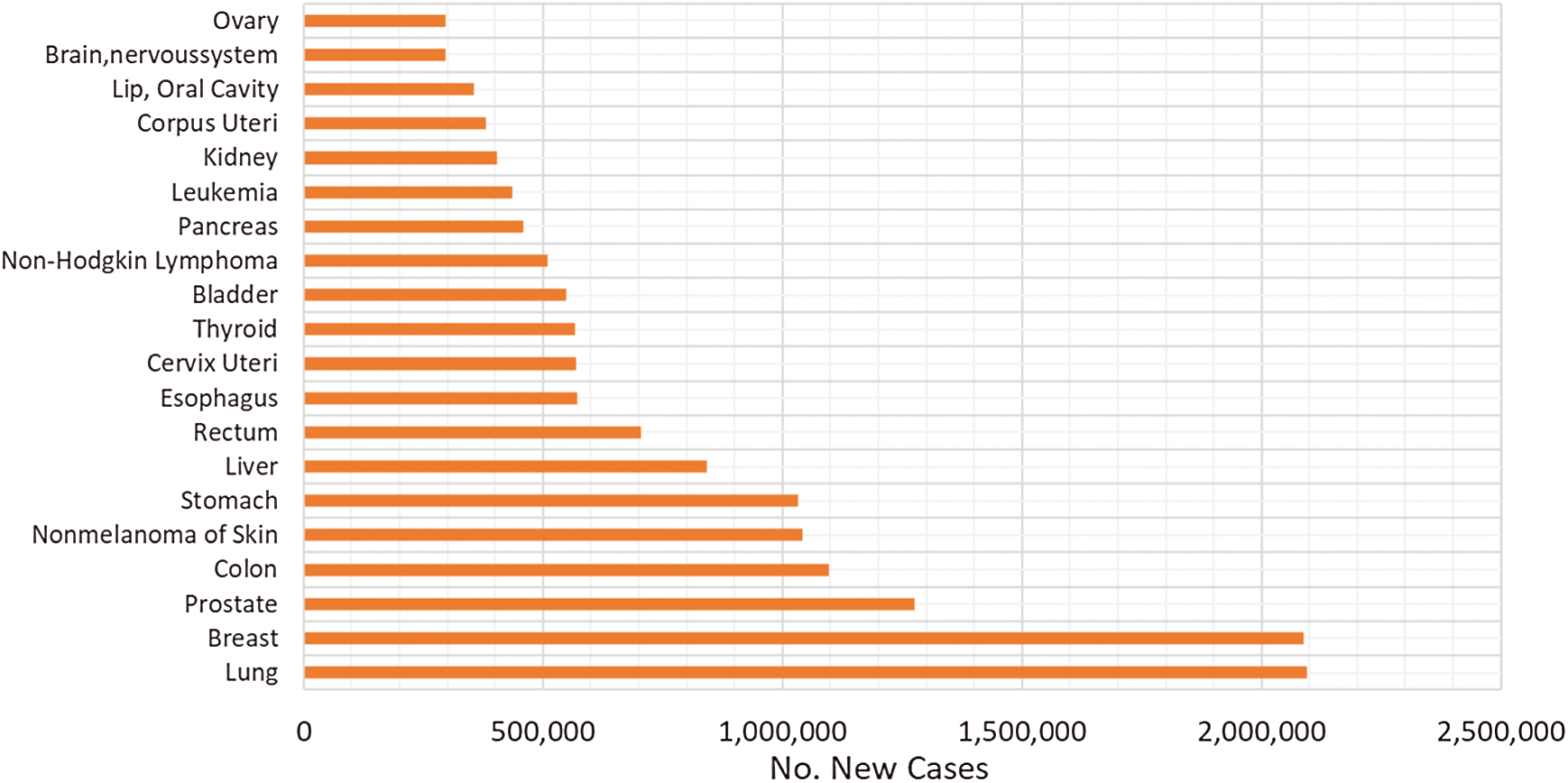
Figure 1: Worldwide incidence of the most frequent cancer types in 2018 [5]
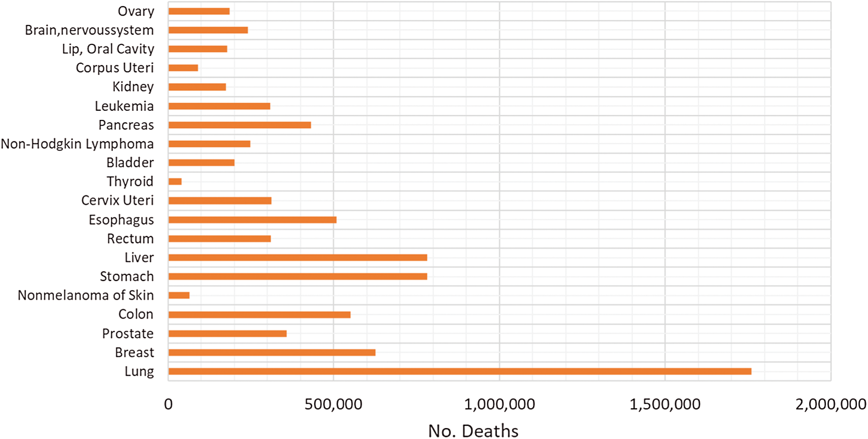
Figure 2: Worldwide number of death cases reported in 2018 [5]
The incidence increment is probably correlated to poor eating habits, obesity and smoking [6]. Fig. 3 shows the estimated incidence of colorectal cancer by country, due to sedentary lifestyle and an unhealthy habits China is in the first place of the list [8], followed by United States with 48 cases per 100,000 inhabitants, in this case the incidence is attributed to obesity alongside with tobacco and alcohol consumption.
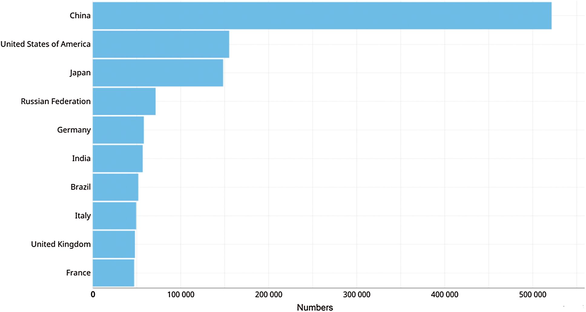
Figure 3: Estimated incidence of colorectal cancer by countries in the year 2018 [5]
Colon cancer diagnosis is more frequent in men than in women in the ages between 50 and 65 years. Since there is no early diagnosis, one out of every four cases will develop metastasis [9,10]. In Japan 86% of individuals diagnosed under the age of 50 were symptomatic at the time of diagnosis, which is directly related to advanced stages and worse prognosis [10,11]. On the other hand, France has a low estimated incidence probably due to its preventive policy in public primary care, including intestinal cancer test by colonoscopy, fecal occult blood and immunological screening [12].
The proprietary dataset used in this paper is from Basque Country in Bilbao Spain. Therefore, the detailed incidence of cancer cases in Spain is presented and summarized in Fig. 4. There were 567.463 new cases detected in 2018, meaning 67 cases per 100,000 inhabitants, and 263,895 deaths due to colorectal cancer, meaning 31 deaths per 100,000 inhabitants. By 2035 it is estimated that there will be 315,413 deceases because of cancer. In particular, there were [13].
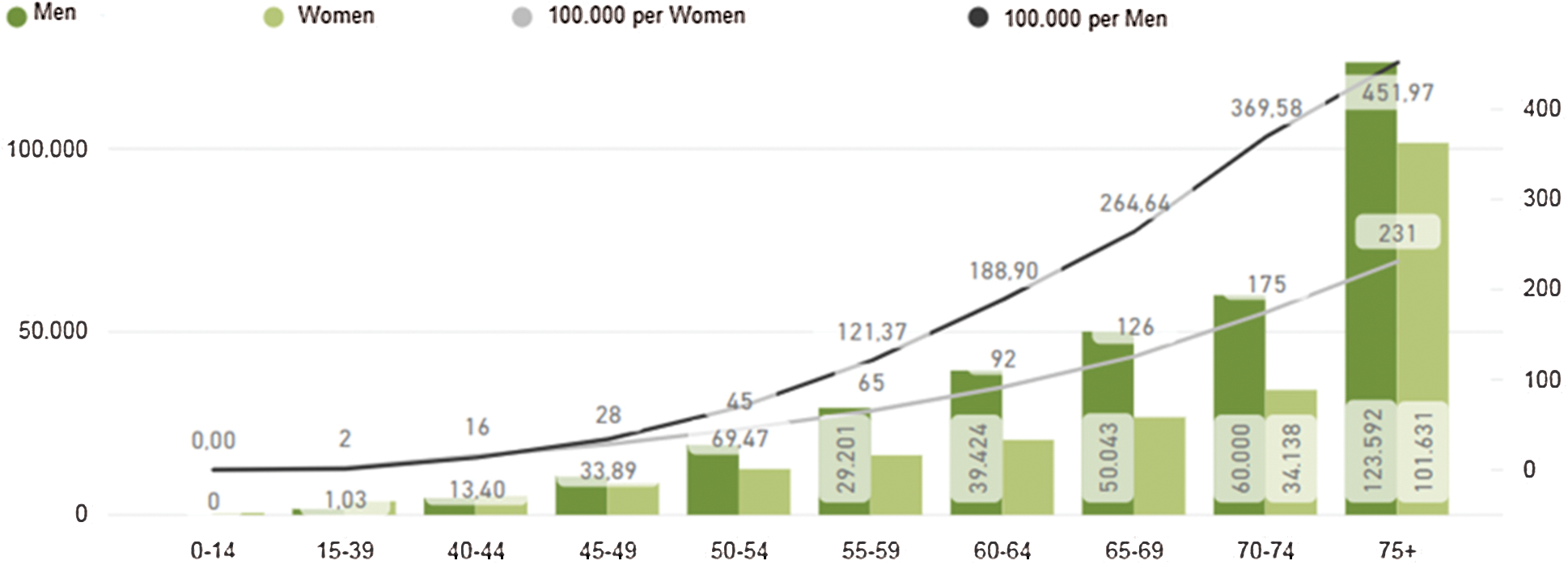
Figure 4: Estimated incidence of colorectal cancer in Spain [13]
Colorectal cancer consists in the apparition of neoplasms or polyps, originated when healthy cells from the inner lining of the colon or rectum change and grow uncontrollably, forming a mass called adenocarcinoma. Most colorectal cancer cases are preceded by diseases such as intestinal polyposis, Peutz–Jegher disease, Lynch syndrome, and inflammatory bowel disease [14]. Polyps are defined as inflammations of the gastrointestinal wall [15]. When diagnosing colorectal cancer the spread of the disease is measured using five stages, that could be also identified using a Deep Learning approach [16]. In stage 0 cancer treatment is usually conducted by removing the polyp through colonoscopy as the cancer is on the inner lining of the colon. In Stage I cancer has not grown outside the colon wall, if the polyp is removed completely no other treatment is needed. In Stage II the cancer grow through the colon wall and surgery to remove the section of the colon with cancer is needed, at this stage some doctors could recommend chemotherapy as an additional treatment. In Stages III and IV chemotherapy is needed, in Stage III colectomy is required to remove cancer areas and nearby lymph nodes, and in Stage IV due to metastases (often to liver) surgery is unlikely, unless it helps to prolong patients live. Early detection in stage 0 through Stage II is important as cancers could be cured with an 80–90% rate [15,17]. There are studies explaining that 1% increase in the detection rate of polyps is associated with a 3% decrease in the incidence interval of colorectal cancer [18].
This article presents the application of different Deep Learning architectures for the automatic detection and segmentation of colon polyps. These techniques are based on images acquired during colonoscopies and allowing early detection of cancer risk. The tests of the proposed algorithm have been made against standard databases, enabling to compare with other published works and against a new database created in the Basque Country in Spain. This evaluation constitutes a fundamental step in the usage of these techniques for a semi-automatic polyp detection framework.
Early detection of colon polyps provides valuable information to assess the risk of developing cancer. This fact has motivated several studies in automatic polyp detection, leading to diagnosis recommendation systems to assist healthcare professionals. We implemented four deep learning techniques to detect and segment polyps in colonoscopy images, and used CVC-CLINIC and ETIS-LARIB databases to compare our results with state-of-the-art techniques. All the models were trained using two GPU Nvidia GeForce GTX Titan X.
To achieve automatic detection of polyps, we compare some of the most recent Convolutional Neural Networks (CNN) architectures for instance segmentation. Four architectures proposed during the last few years based on their performance on the Microsoft COCO dataset were selected [19]. All predictions are filtered based on their confidence and merged to generate a single binary mask.
This technique is an extension of Faster R-CNN, adding a branch to predict segmentation masks and refining the Region of Interest (RoI) pooling. A Convolutional Neural Network (CNN) is employed to extract image features, from those features another CNN propose RoIs. Then this information is feed to fully connected layers to determine the boundary box from the required elements. Mask R-CNN adds a branch with two extra convolution layers for predicting the actual segmentation masks from each of the ROIs [20]. Additionally, in Mask R-CNN proposal the authors refined the RoI pooling, making every target cell the same size and calculating the feature maps within them by interpolation, this improves the accuracy significantly. In Fig. 5 the neural network flow is presented, ResNet-101 with ImageNet pre-trained weights is used as backbone for feature map extraction over the polyp images, then these feature maps are aligned with the RoIs and feet into fully connected layers (FC) and to additional convolutional layers to perform boundary box predictions and classification on the FC layers and segmentation mask prediction on the convolutional branch. The neural network architecture used in the convolutional layers has  dimensions, and a ReLU activation function was used in the hidden layers. On the presented experiments we used a learning rate of 0.001, learning momentum of 0.9 and weight decay of 10−4.
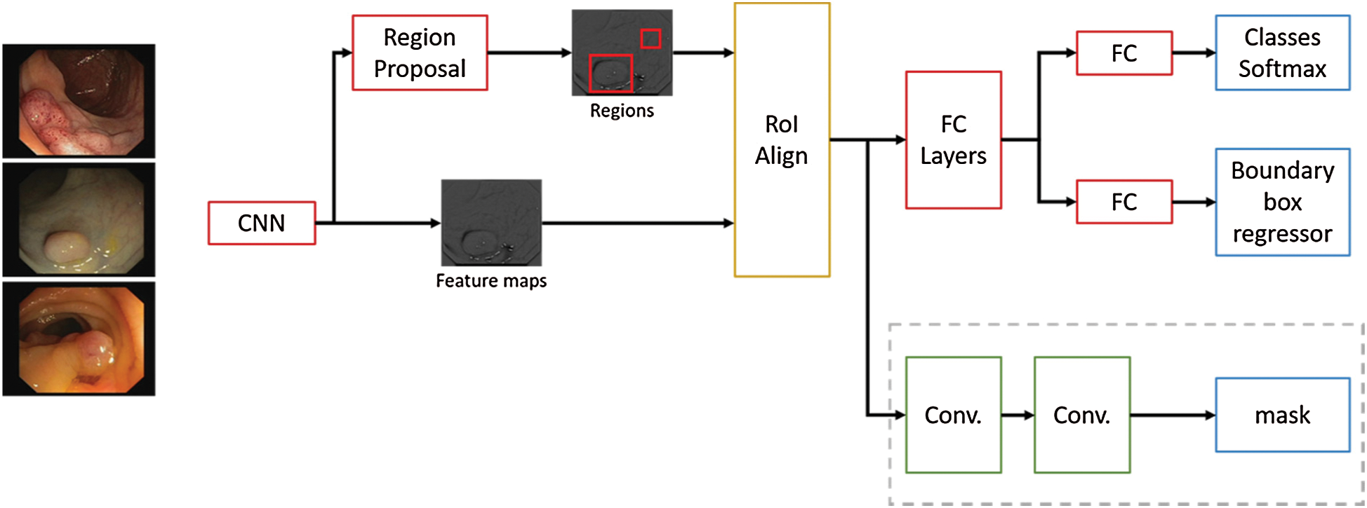
Figure 5: Mask R-CNN network flow for polyp region segmentation
In the previous architecture [20], the authors explore the usage of a Feature Pyramid Network (FPN) on the backbone of the Mask R-CNN network. In their experiments, they found a noticeable increment in their metrics over other architectures. In PANet [21], the authors improve on this architecture enhancing information propagation between low-level and high-level features. In order to achieve this, they propose the usage of a bottom-up augmentation path to propagate low-level features. On each stage of this processes the feature maps of previous stages use a  convolutional layer and adds it to the current one using a lateral connection. Like Mask R-CNN, these maps pass through a RoIAlign layer in order to pool feature grids from each level. Then, they are concatenated using a fusion operation such as element-wise max or element-wise sum in what is called an adaptive feature pooling layer, this architecture is described in Fig. 6. Finally, the authors of this method improved mask prediction adding a fully connected layer that gets concatenated to the final convolutional layer, which generates the final mask.
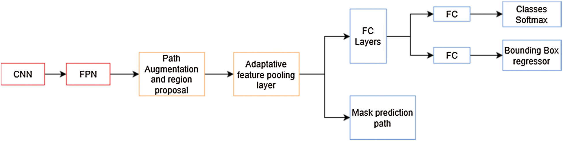
Figure 6: PANet architecture overview. The mask prediction path is similar to the one in mask R-CNN in Fig. 5
ResNext-101 pre-trained with ImageNet [22] was used as the feature extractor for this architecture. We employ Stochastic Gradient Descent (SGD) as optimizer with momentum of 0.9 and a weight decay of 10−4. We use a learning rate of 0.01 with 500 iterations of gradual warm up. In order to fit batches of 8 images in memory, we rescale the images to  pixels, except the ones from ClinicDB that have lower resolution. We trained the neural network for 20 iterations and selected the optimal epoch in order to avoid overfitting the datasets.
In [23] the authors presented a method for training and evaluating models based on the Faster R-CNN framework, which uses an IoU threshold of 0.5 to filter proposed bounding boxes, limiting the performance of deep learning algorithms. This can be attributed to the lack of incentive for the model to predict more accurate bounding boxes, and that using a higher IoU makes it harder for the model to obtain initial results over which to improve. As presented in Fig. 7, to solve this problem, the authors propose a modification to Faster R-CNN framework which include a multi-stage extension of the original architecture. They used a combination of cascaded bounding box regressions and cascaded detection. With this technique, the model is able to progressively refine its prediction, sampling the training data with increasing IoU thresholds on each stage. This allows the model to handle different training distributions.
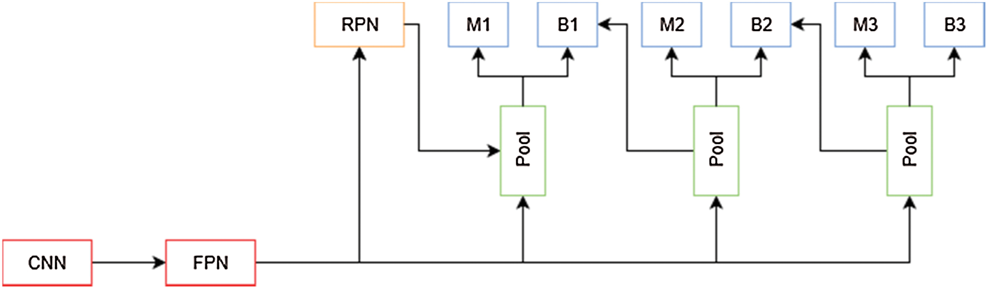
Figure 7: Cascade mask R-CNN architecture overview. M is a mask predictor and B is a bounding box predictor
The architecture selected as network backbone is ResNext-101 pre-trained with ImageNet database. For the experiments we employed SGD as optimizer with momentum of 0.9, weight decay of 10−4 and again we rescale the images to  pixels, except the ones from ClinicDB, in order to fit them in memory for a batch size of 8. We use a learning rate of 0.005 with a warm-up of 500 iterations. We trained the neural network for 20 iterations and selected the most optimal epoch in order to avoid overfitting the datasets.
2.1.4 Hybrid Task Cascade (HTC)
The advantages of cascade models for image segmentation were explored by [23], which resulted in Cascade Mask R-CNN, but [24] argue that this is not an optimal way of leveraging the improvements that a cascade model can provide. To improve Cascade Mask R-CNN results, the authors propose a new cascade architecture (Fig. 8) that interleaves the bounding box and mask prediction branches, so that the latter can take advantage of the updated bounding box predictions. Another addition is the inclusion of a segmentation mask. This layer connected to the output of the Feature Pyramid is used as a complementary task that improves performance when trained fused with the bounding box and mask features.
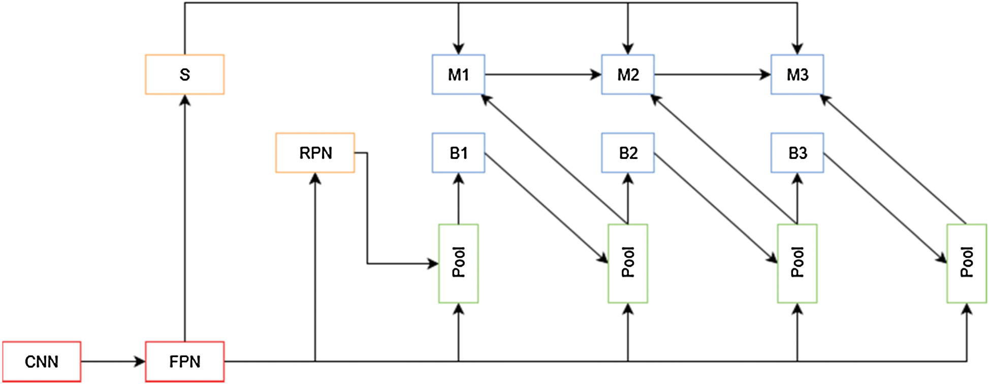
Figure 8: HTC network overview. S is the segmentation path for this architecture
The architecture selected as the network backbone is ResNext-101 pre-trained with ImageNet database. For the experiments we employ SGD with momentum of 0.9, weight decay of 10−4 and we rescale the images to  pixels, except the ones from ClinicDB. in order to fit them in memory for a batch size of 8. We use a learning rate of 0.005 with a warm up of 500 iterations. We trained the neural network for 20 iterations and selected the most optimal epoch in order to avoid overfitting the datasets.
Colonoscopy is the reference method for the diagnosis and treatment of colonic diseases. It is an exploratory technique that allows the assessment of the colon wall through endoscopic examination. The lesions detected are assessed to be removed and biopsies are taken for analysis. One of the main problems arising in the colon are polyps, these are abnormal tissue growths appear in the intestinal mucous membrane. They normally occur in between 15% and 20% of the adult population, being one of the most common problems affecting the colon and rectum. Even though most polyps are benign, their association with colorectal cancer has been proven, develop via the adenoma-carcinoma sequence [25]. As it can be seen in Fig. 9, in order to detect Polyps on colonoscopy screening three challenges should be addressed [26]:
• There are a variety of noises on the images known as artifacts, such as specular highlights, lens frames and inadequate preparation for the procedure.
• Polyps have a number of shapes and textures and they can vary from 3 mm to 10 mm.
• There are transformation and distortions from the employed imaging system.
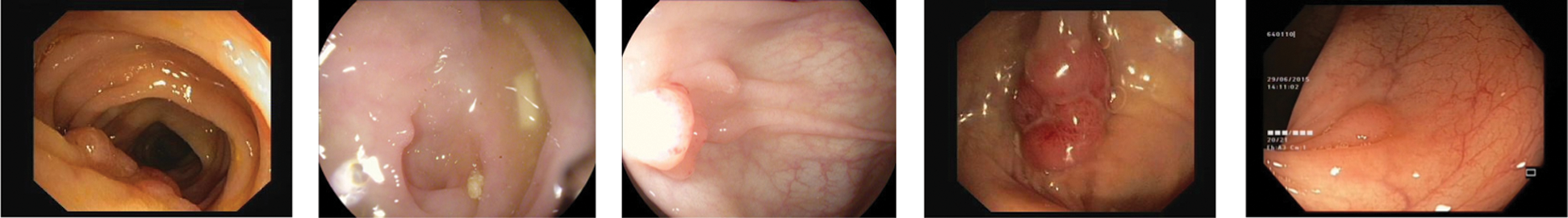
Figure 9: Different polyp shapes and artifacts present in colonoscopy images make difficult their segmentation
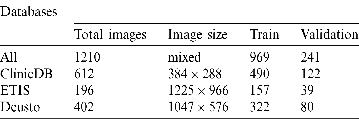
Several computer-aided techniques have been proposed to detect polyps in colonoscopies [27]. We used two public databases and one proprietary database to detect and segment colon polyps. All our experiments were trained and validated using these 3 databases: CVC-ClinicDB database and ETIS-LARIB Polyp from the 2015 MICCAI sub-challenge on automatic polyp detection [28] and one proprietary database from Deusto University e-Vida research group. Tab. 1 contains the number of images, image size and train and validation subset sizes, in the first column the combination from the 3 databases is called all and contains images with different sizes.
We conducted three sets of experiments in order to evaluate the performance of the proposed techniques when tested with different databases. The experimental set up is presented in Fig. 10, in the first experiment we compared the results when training the model by using each of the databases independently and test on independent evaluation sets, in the second experiment we used the training sets from the three databases for training and tested on each testing set from the databases independently, adding one testing set formed from the conjunction of the three databases. Finally, we trained on each database independently and tested on an expanded testing set formed by the conjunction of the three databases. On each of the experiments we employed an 80/20 training/test ratio.
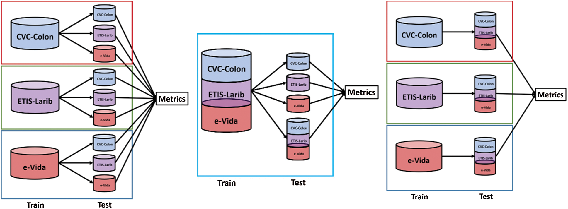
Figure 10: Experiments designed to test the performance of the proposed techniques by using 3 databases
To measure segmentation, we compare the binary mask generated by our model with the ground truth pixel by pixel. The metrics used for testing the segmentation performance are presented in Tab. 2. These metrics are defined in terms of the correct detection output for the cases that are inside the polyp region (True Positive), the detection output of polyps for cases outside the polyp in the ground truth (False Positive), polyp not detected in a region containing a polyp in the ground truth (False Negative), and no detection in a region without polyp in the ground truth (True Negative). These regions are described in Fig. 11, the overlap of regions is defined as True Positive, the missing detection of the ground truth are False Positive, the incorrect detection is False Positive, anything falling outside these regions are the True Negative cases.
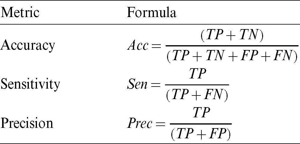
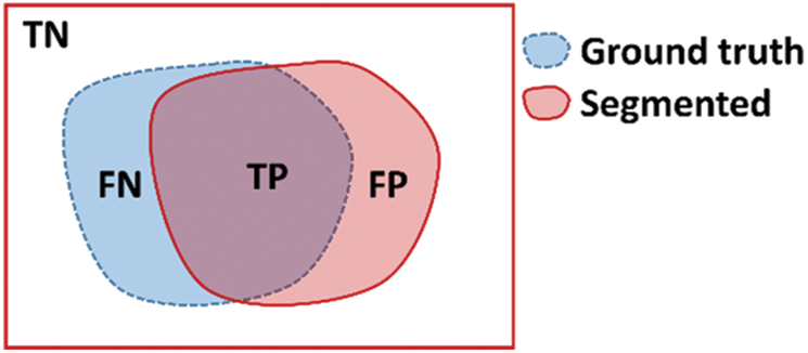
Figure 11: Region definition for TN: True Negative, FN: False Negative, TP: True Positive, and FP: False Positive
The results of the application of multiple Deep Learning models are presented in two sections, we present both the detection rate of polyps and the segmentation performance from the technique.
The polyp detection rate for the implemented techniques is presented in Tabs. 3–6. These tables summarize the error results of the three experiments proposed, the error is measured as the ratio between the detected polyp and the actual presence of a polyp on the image. The best performance is obtained when the model was trained using all databases and testing on Deusto database as highlighted in green. Additionally, we highlight for each database used in training, the best test result in bold. As observed the lowest error percentage is achieved when training with all datasets and testing on the Deusto data. ETIS dataset is relatively small and therefore, as expected, has more error in detection on average for all models.
Table 3: Mask R-CNN polyp detection rate
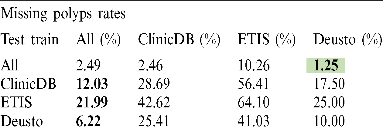
Table 4: PANet polyp detection rate
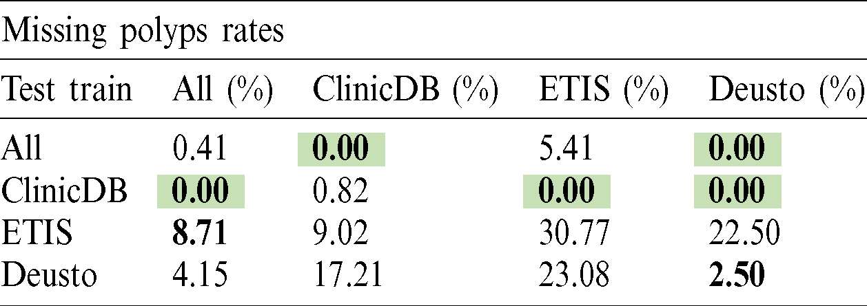
Table 5: Cascade R-CNN polyp detection rate

Table 6: HTC polyp detection rate

Tabs. 7–10 present the metrics results for the polyp segmentation when using the proposed techniques for polyp detection. The best performances for each of the metrics are highlighted in green, while the best performance for each of the databases are highlighted by using bold fonts. We note that training on all databases provides an overall advantage although it may not necessarily lead to the best performance in each metric.
Table 7: Mask R-CNN polyp segmentation rates

Table 8: PANet polyp segmentation rates

Table 9: Cascade R-CNN polyp segmentation rates

Table 10: HTC polyp segmentation rates

Even though few authors have explored the problem of polyp segmentation, multiple works on polyp detection and localization have been made in recent years. Most remarkable results have been obtained exploring the use of deep learning and end to end models instead of hand-crafted solutions, as it can be seen on the results of the 2015 MICCAI sub-challenge on automatic polyp detection [28].
To identify how relevant our results in segmentation are, the model is compared with the lowest polyp missing rate trained with ClinicDB and tested using ETIS against past results reported. In Tab. 11 we show the results of the two best models in the MICCAI competition, and their combination [28]. We also include the results of two previous works that used fully convolutional networks for this problem. One of them experimented with multiple well-known architectures such as GoogLeNet and VGG [29] and the other used a model based on Faster R-CNN with two types of image augmentation for increased accuracy [27].
Table 11: Segmentation metrics

For this comparison, the best models were included respectively (FCN-VGG, and Faster-CNN with Aug1 and with Aug2). Our results were adapted to the previously reported metrics based on the Intersection-over-Union (IoU) in the following way, using an IoU threshold of 0.5:
• True Positive (TP): The model made an accurate prediction of the location of a polyp. We mark with this label the prediction if the IoU between the output of our model and the ground truth is greater or equal than 0.5.
• False Positive (FP): The model predicted a polyp in the wrong location, or its segmentation mask covered an area much bigger or much smaller than the true area of the polyp. We use this label when the IoU is lower than 0.5 and gave a prediction.
• False Negative (FN): The model did not predict a mask when there is at least a polyp on the image. We only considered this label when none of the predictions of the network make past the confidence threshold and the model outputs an empty binary mask.
With this, we calculate precision, recall and F1 metrics. To obtain more precise polyp localizations we also test a higher confidence threshold to filter more detections, which in return lowers our recall. In both cases we tested the model trained using the ClinicDB dataset with all images from the ETIS dataset and not only those separated for validation.
In this paper the application of four deep learning models for the detection and segmentation of polyps in colonoscopy images was presented. These models were trained and tested using three data bases: CVC-CLINIC, ETIS-LARIB and a proprietary database from Deusto University. In order to evaluate the performance three experiments were conducted and discussed. The results were obtained and compared when using each database independently, combining them for training and for testing the models. It should be noted that these databases contain images with different resolutions and characteristics, which allowed us to demonstrate the model capabilities on a real deployment environment. The results for both the polyp detection rate and the segmentation were presented, the best detection rate was obtained when training the model with all the databases and using PANet architecture, the best segmentation accuracy (98.17%) was obtained when using HTC architecture trained with the merged dataset and tested on CVC-CLINIC database. The results obtained from the training and testing with the combined datasets are promising, we are currently working on a framework for real time processing of live feed from colonoscopy, integrating these techniques for the colon polyp detection and segmentation, with the Kudo’s classification of the findings, to generate an alert system to aid the medical personnel. providing computer-aided diagnosis of risk. We foresee that the presented method can be used to provide a robust semi-automated polyp detection and segmentation tool.
Acknowledgement: The authors would like to thank to Hospital Universitario Donostia (Inés Gil and Luis Bujanda), Hospital Universitario de Cruces (Manuel Zaballa and Ignacio Casado), Hospital Universitario de Basurto (Angel José Calderón and Ana Belen Díaz), Hospital Universitario de Araba (Aitor Orive and Maite Escalante), Hospital de San Eloy (Fidencio Bao and Iñigo Kamiruaga) and Hospital Galdakao (Alain Huerta) health centres and Osakidetza Central (Isabel Idígoras and Isabel Portillo) for their collaboration in the research.
Funding Statement: This research was supported by the Basque Government “Aids for health research projects” and the publication fees supported by the Basque Government Department of Education (eVIDA Certified Group IT905-16).
Conflicts of Interest: The authors declare that they have no conflicts of interest to report regarding the present study.
1. Observatorio AECC. (2020). “Cáncer de colon en cifras,” . [Online]. Available: http://observatorio.aecc.es/. [Google Scholar]
2. A. Sanchez-Gonzalez, B. Garcia-Zapirain, D. Sierra-Sosa and A. Elmaghraby. (2018). “Automatized colon polyp segmentation via contour region analysis,” Computers in Biology and Medicine, vol. 100, pp. 152–164. [Google Scholar]
3. R. L. Siegel, K. D. Miller and A. Jemal. (2019). “Cancer statistics, 2019,” CA: A Cancer Journal for Clinicians, vol. 69, no. 1, pp. 7–34. [Google Scholar]
4. F. Bray, J. Ferlay, I. Soerjomataram, R. L. Siegel, L. A. Torre et al. (2018). , “Global cancer statistics 2018: GLOBOCAN estimates of incidence and mortality worldwide for 36 cancers in 185 countries,” CA: A Cancer Journal for Clinicians, vol. 68, no. 6, pp. 394–424. [Google Scholar]
5. World Health Organization. (2018). “Latest global cancer data: Cancer burden rises to 18.1 million new cases and 9.6 million cancer deaths in 2018.” Technical Report September, International Agency for Research on Cancer, Press Release N02070; 263, . https://www.who.int/cancer/PRGlobocanFinal.pdf. [Google Scholar]
6. J. Ferlay, M. Colombet, I. Soerjomataram, T. Dyba, G. Randi et al. (2018). , “Cancer incidence and mortality patterns in Europe: Estimates for 40 countries and 25 major cancers in 2018,” European Journal of Cancer, vol. 103, pp. 356–387. [Google Scholar]
7. Observatorio del Cáncer de la AECC. (2018). “Incidencia y Mortalidad de Cáncer colorrectal en España en la población entre 50 y 69 años,” . [Online]. Available: https://www.aecc.es/sites/default/files/content-file/Informe-incidencia-colon.pdf. [Google Scholar]
8. M. J. Gu, Q. C. Huang, C. Z. Bao, Y. J. Li, X. Q. Li et al. (2018). , “Attributable causes of colorectal cancer in China,” BMC Cancer, vol. 18, no. 1, pp. 38. [Google Scholar]
9. CDC. (2013). “United States Cancer Statistics 2013,” . [Online]. Available: https://www.cdc.gov/cancer/uscs/pdf/uscs-2013-technical-notes.pdf. [Google Scholar]
10. A. Rico, L. A. Pollack, T. D. Thompson, M. C. Hsieh, X. C. Wu et al. (2016). , “KRAS testing and first-line treatment among patients diagnosed with metastatic colorectal cancer using population data from ten National Program of Cancer Registries in the United States,” Journal of Cancer Research & Therapy, vol. 5, no. 2, pp. 7. [Google Scholar]
11. A. Tamakoshi, K. Nakamura, S. Ukawa, E. Okada, M. Hirata et al. (2017). , “Characteristics and prognosis of Japanese colorectal cancer patients: The BioBank Japan project,” Journal of Epidemiology, vol. 27, no. 3, pp. S36–S42. [Google Scholar]
12. World Health Organization. (2014). “Cancer country profiles,” . [Online]. Available: https://www.who.int/cancer/country-profiles/irn_en.pdf. [Google Scholar]
13. Sociedad Española de Oncología Médica. (2018). “Las Cifras del Cáncer en España 2018,” . [Online]. Available: https://seom.org/seomcms/images/stories/recursos/Las_Cifras_del_cancer_en_Espana2018.pdf. [Google Scholar]
14. R. Prado, J. Lahsen and J. Hernández. (2008). “Síndrome de Peutz-Jeghers complicado: Reporte de un caso,” Revista Chilena de Cirugía, vol. 60, no. 3, pp. 249–254. [Google Scholar]
15. F. Arévalo, V. Aragón, J. Alva, M. Perez Narrea, G. Cerrillo et al. (2012). , “Pólipos colorectales: Actualización en el diagnóstico,” Revista de Gastroenterología del Perú, vol. 32, no. 2, pp. 123–133. [Google Scholar]
16. S. Patino-Barrientos, D. Sierra-Sosa, B. Garcia-Zapirain, C. Castillo-Olea and A. Elmaghraby. (2020). “Kudo’s classification for colon polyps assessment using a deep learning approach,” Applied Sciences, vol. 10, no. 2, pp. 501. [Google Scholar]
17. U. A. Gualdrini, A. Sambuelli, M. Barugel, A. Gutiérrez and K. C. Ávila. (2005). “Prevención del cáncer colorrectal (CCR),” Acta Gastroenterológica Latinoamericana, vol. 35, no. 2, pp. 104–140. [Google Scholar]
18. R. J. Barnard. (2004). “Prevention of cancer through lifestyle changes,” Evidence-Based Complementary and Alternative Medicine, vol. 1. [Google Scholar]
19. T. Y. Lin, M. Maire, S. Belongie, J. Hays, P. Perona et al. (2014). , “Microsoft coco: Common objects in context,” in European Conf. on Computer Vision, Zurich, Switzerland, Cham: Springer, pp. 740–755. [Google Scholar]
20. K. He, G. Gkioxari, P. Dollár and R. Girshick. (2017). “Mask R-CNN,” in Proc. of the IEEE Int. Conf. on Computer Vision, pp. 2961–2969. [Google Scholar]
21. S. Liu, L. Qi, H. Qin, J. Shi and J. Jia. (2018). “Path aggregation network for instance segmentation,” in Proc. of the IEEE Conf. on Computer Vision and Pattern Recognition, pp. 8759–8768. [Google Scholar]
22. O. Russakovsky, J. Deng, H. Su, J. Krause, S. Satheesh et al. (2015). , “Imagenet large scale visual recognition challenge,” International Journal of Computer Vision, vol. 115, no. 3, pp. 211–252. [Google Scholar]
23. Z. Cai and N. Vasconcelos. (2018). “Cascade r-cnn: Delving into high quality object detection,” in Proc. of the IEEE Conf. on Computer Vision and Pattern Recognition, Venice, Italy, pp. 6154–6162. [Google Scholar]
24. K. Chen, J. Pang, J. Wang, Y. Xiong, X. Li et al. (2019). , “Hybrid task cascade for instance segmentation,” in Proc. of the IEEE Conf. on Computer Vision and Pattern Recognition, Long Beach, California, pp. 4974–4983. [Google Scholar]
25. D. W. Day and B. C. Morson. (1978). “The adenoma-carcinoma sequence,” Major Problems in Pathology, vol. 10, pp. 58–71. [Google Scholar]
26. X. Mo, K. Tao, Q. Wang and G. Wang. (2018). “An efficient approach for polyps detection in endoscopic videos based on faster R-CNN,” in 24th Int. Conf. on Pattern Recognition (ICPR) IEEE, Beijing, China, pp. 3929–3934. [Google Scholar]
27. Y. Shin, H. A. Qadir, L. Aabakken, J. Bergsland and I. Balasingham. (2018). “Automatic colon polyp detection using region based deep cnn and post learning approaches,” IEEE Access, vol. 6, pp. 40950–40962. [Google Scholar]
28. J. Bernal, N. Tajkbaksh, F. J. Sánchez, B. J. Matuszewski, H. Chen et al. (2017). , “Comparative validation of polyp detection methods in video colonoscopy: Results from the MICCAI, 2015 endoscopic vision challenge,” IEEE Transactions on Medical Imaging, vol. 36, no. 6, pp. 1231–1249. [Google Scholar]
29. P. Brandao, E. Mazomenos, G. Ciuti, R. Caliò, F. Bianchi et al. (2017). , “Fully convolutional neural networks for polyp segmentation in colonoscopy, Computer-Aided Diagnosis,” Medical Imaging, vol. 10134, 101340F. [Google Scholar]
 | This work is licensed under a Creative Commons Attribution 4.0 International License, which permits unrestricted use, distribution, and reproduction in any medium, provided the original work is properly cited. |