A Cyber Kill Chain Approach for Detecting Advanced Persistent Threats

Yussuf Ahmed; A.Taufiq Asyhari; Md Rahman

doi:10.32604/cmc.2021.014223

1School of Computing and Digital Technology, Birmingham City University, Birmingham, UK
2Faculty of Computing, IBM CoE, ERAS, University Malaysia Pahang, Pahang, Malaysia
*Corresponding Author: Yussuf Ahmed. Email: yussuf.ahmed@bcs.org
Received: 07 September 2020; Accepted: 13 December 2020

Abstract: The number of cybersecurity incidents is on the rise despite significant investment in security measures. The existing conventional security approaches have demonstrated limited success against some of the more complex cyber-attacks. This is primarily due to the sophistication of the attacks and the availability of powerful tools. Interconnected devices such as the Internet of Things (IoT) are also increasing attack exposures due to the increase in vulnerabilities. Over the last few years, we have seen a trend moving towards embracing edge technologies to harness the power of IoT devices and 5G networks. Edge technology brings processing power closer to the network and brings many advantages, including reduced latency, while it can also introduce vulnerabilities that could be exploited. Smart cities are also dependent on technologies where everything is interconnected. This interconnectivity makes them highly vulnerable to cyber-attacks, especially by the Advanced Persistent Threat (APT), as these vulnerabilities are amplified by the need to integrate new technologies with legacy systems. Cybercriminals behind APT attacks have recently been targeting the IoT ecosystems, prevalent in many of these cities. In this paper, we used a publicly available dataset on Advanced Persistent Threats (APT) and developed a data-driven approach for detecting APT stages using the Cyber Kill Chain. APTs are highly sophisticated and targeted forms of attacks that can evade intrusion detection systems, resulting in one of the greatest current challenges facing security professionals. In this experiment, we used multiple machine learning classifiers, such as Naïve Bayes, Bayes Net, KNN, Random Forest and Support Vector Machine (SVM). We used Weka performance metrics to show the numeric results. The best performance result of 91.1% was obtained with the Naïve Bayes classifier. We hope our proposed solution will help security professionals to deal with APTs in a timely and effective manner.

Keywords: Advanced persistent threat; APT; Cyber Kill Chain; data breach; intrusion detection; cyber-attack; attack prediction; data-driven security and machine learning

In the last few years, we have seen the growth in the scale and complexity of cyber-attacks targeting organizations. A global report by IBM [1] showed that the average cost of a cyber-breach was found to be $3.86 million. One of the most sophisticated attacks utilized by cybercriminals is Advanced Persistent Threat (APT), whose goal is to gain unauthorized access, maintain a foothold and exfiltrate or modify data. APTs are targeted and persistent forms of attack and may go unnoticed for an extended timescale [2]. According to FireEye, the global median dwell time of APT attacks is 56 days [3]. APT attackers often use multiple attack vectors to obtain or modify the information, which is even made easier by the ever-expanding attack surface in the digitized world. For example, cybercriminals could exploit devices ranging from the Internet of Things (IoT), smart cameras, and Bring Your Own Devices (BYOD), which are present in most organizations.

In recent times we have also observed a remarkable increase in the number of remote users due to the Covid19 pandemic. Cybercriminals are using every opportunity to take advantage of this surge in remote working. They employ techniques such as phishing attacks to exploit unsuspecting users and to compromise previously secure networks. Attackers could also exploit internet-facing open ports on home routers with default credentials to compromise the remote users, causing a cascading effect on the infrastructure using the stolen credentials. According to a recent report by a leading UK Privileged Access Management (PAM) provider [4], 71% of the surveyed decision-makers believed the arrangement of remote working during the Covid-19 pandemic magnified the probability of a cyber-breach. APT attacks are mostly utilized by organized cyber criminals but there are also large security breaches linked to nation-state actors with the aims of espionage and attacks on national critical infrastructure.

According to a Verizon Data Breach Investigation Report [5], there was an increase in cyber espionage involving APTs using a combination of phishing and malware. According to another report by Malwarebytes [6], organized criminals and nation-state actors linked APT groups have been using coronavirus-based phishing attacks to compromise and gain a foothold on the victim machines [7]. The attack vectors used include template injection, malicious macros, and linked files, while others have used malicious attachments supposedly containing Covid19 prevention measures [8].

Recent interests have shown an increased focus to deal with APT attacks. A variety of cybersecurity measures and methodologies have been investigated to detect, monitor, and mitigate the APTs, and their impacts. Conventional cybersecurity approaches have demonstrated some limited success at detecting APTs due to their sophistication, and when they are detected, they tend to adapt very quickly and change course. Most of the APT groups are well resourced and will try every effort to achieve their goal. These motivate the recent development of machine learning and computational intelligence techniques to improve the detection of the APTs, which can then translate into timely intervention measures.

While several predecessor works have investigated machine learning for APT detection and mitigation, there have been various shortcomings in their effectiveness for wider uses. These include: (i) a lack of reliable publicly-open APT datasets, (ii) a lack of alignment with Industry-informed practice on the available dataset construction, (iii) limited experimental works to evaluate the learning algorithm effectiveness. This work proposes to advance the machine learning application for APT detection by addressing the latter two shortcomings from the previous works. Our main contributions include:

• Building upon a recently proposed APT dataset in [9], we leverage an industry-informed framework of Cyber Kill Chain to reconstruct a dataset that captures realistic APT stages. Through this dataset reconstruction, we employ data intelligence via machine learning that exploits possible patterns within the reconstructed dataset.

• Given the limited number of features in the original APT dataset, we perform feature extraction via multi-factor analysis (MFA) that creates abstract features to provide options for training machine learning models in the APT stage detection and classification.

• To improve the classification accuracy, we investigate feature selection techniques to remove noisy and less relevant features for APT stage detection and classification. A different number of selected features are assessed to provide optimal tuning to the overall machine learning models.

• Using baseline machine learning classifiers, we perform in-depth and rigorous analysis of the experimental results and assess the trade-off of the classifiers’ performance using a variety of performance metrics.

This work improves the work in [9] by using the industry-informed Cyber Kill Chain approach for dataset reconstruction for enhancing the resolution on the attack stages and alert types, which are critical in the APT attack analysis. To prevent a direct linkage between an attack stage and an alert type as found in [9], we carefully refine the alerts grouping with one alert possibly corresponding to multiple attack stages as informed by the APT lifecycle within the Cyber Kill Chain framework. This may inevitably reduce the ability to perform accurate stage classification. For improving the APT detection accuracy, we conduct feature extraction and selection before APT stage classification. For the subsequent sections of the paper, we will refer to the work in [9] as the APT dataset provider.

The rest of this paper is organized as follows. Section 2 discusses closely related works and how they shape our current work. Section 3 applies the Cyber Kill Chain to cybersecurity data modeling. Section 4 discusses our machine learning construction to classify the APT attack stages based on the Cyber Kill Chain informed data model. Section 5 explains the experiments to validate the effectiveness of the machine learning model covered in Section 4. Section 6 concludes the paper by highlighting important points in this work and setting up future research direction.

Most of the information available on APTs is from the industry, although some research was carried out in the academic circles. The extensive research by industry leaders such as FireEye [10] and Kaspersky [11] led to the discovery of many APTs, including those used by nation-state actors that are difficult to detect. For example, FireEye published research on APT41, which is linked to nation-state actors and used for espionage and financial gains [12]. Several industry leaders proposed attack Life Cycle frameworks for dealing with cyber threats. These frameworks include the Lockheed Martin Cyber Kill Chain, the Diamond model, Mandiant Attack Life Cycle, and MITRE ATT&CK model.

The Lockheed Martin Cyber Kill Chain has seven stages covering the whole attack life cycle and is the primary focus of our research. The Diamond model is another approach for detecting intrusion and has four interconnected features that are present in every attack. These features are adversary, capability, infrastructure, and victim. The Mandiant attack life cycle consists of multiple components mapped to the various phases of the attack life cycle. The industry research has its own limitations, given they are not peer-reviewed and are mostly used as a platform to market their products. APT attacks have also been gaining interest from academic researchers, and several authors have published articles on this subject. In [13], the authors surveyed APTs and proposed a taxonomy for APT defense classification. Similarly, [14] carried a survey on APTs and reviewed some of the known APT groups’ activities but did not cover defensive or detective technical measures. This work mostly relied on publicly available data on APTs shared by the industry, although they described such sources’ limitations.

Another APT attack life cycle methodology was proposed in [15]. The authors proposed four stages which were, prepare, access, resident, and harvest. In the preparation stage, the attackers gather information relating to the target. The access and harvest stages broadly encompass the step involved in compromising the target. According to the authors, the most common attack vectors for APT include watering hole and spearfishing. In [16], the authors discussed the tools and techniques available to the attackers and linked them to the various stages of the Cyber Kill Chain, but the review was more generic. It could have benefited from evaluating certain APT attacks or groups. Similarly, in [17], the author proposed a taxonomy for banking Trojans based on the Cyber Kill Chain. In another work [18], the authors leveraged the Cyber Kill Chain to break-down complex attacks and built a picture of the APT attackers’ tactics, techniques, and procedures (TTPs). The authors analyzed over 40 APTs to build their proposed taxonomy.

As mentioned in Section 1, the original APT dataset provider proposed a machine learning-based framework for APT detection and proposed six APT steps; however, they only considered four of these as detectable APT attack stages. These stages are (i) Point of entry, (ii) C&C communication, (iii) Asset/data recovery, (iv) Data exfiltration. Their MLAPT framework consists of three phases: threat detection, alert correlation, and attack detection. Their proposed detection modules are Disguised exe File Detection (DeFD), Malicious File Hash Detection (MFHD), Malicious Domain Name Detection (MDND), Malicious IP Address Detection (MIPD), Malicious SSL Certificate Detection (MSSLD), Scanning Detection (SD) and Tor Connection Detection (TorCD) as in Fig. 1.

In [19], the authors proposed an approach for detecting APT using fractal methods based on a k-NN algorithm, which, according to the authors, resulted in a reduction in false positives and false negatives. In a similar report [20], the authors performed experiments to detect the stages of APT attacks. They used the NSL-KDD dataset and selected Principal Component Analysis (PCA) for feature sampling.

In [21], the author categorized the APT attack lifecycle into five phases: reconnaissance, compromise, maintaining access, lateral movement, and data exfiltration. In [22], the authors categorized APT phases into reconnaissance, delivery, exploitation, operation, data collection, and exfiltration and proposed an APT detection methodology.

Reference [23] studied a conceptual framework for APT detection, building on the work by the APT dataset provider. Their proposed solution is a work in progress and did not contain experiments and results to demonstrate their proposed framework’s effectiveness. We differ from their work significantly because we performed experiments using the APT dataset, reconstructed the dataset, and performed feature extraction, feature selection, and classification along with detailed analysis of the results.

Despite the recent progress in APT research, the existing works are mostly hampered by the lack of datasets on APT. Most of the current research relies on old datasets that might not reflect on the current sophistication of the attacks. There are few initiatives for sharing data, such as the Veris framework [24] but even then, the data could be heavily anonymized. Furthermore, there is limited experimental evidence of explicit association and linkage between existing APT datasets and the corresponding machine learning with the Cyber Kill Chain data modeling.

In this research, we attempt to address these aforementioned technical gaps by reconstructing the recently proposed APT dataset, as mentioned in Section 1, through the Cyber Kill Chain modeling and mapping approach. Based on the reconstructed dataset, we next design and develop machine learning models to intelligently learn from the dataset. We then conduct rigorous experiments and analysis of the results to gain insights into the accuracy of the machine learning models and other relevant performance metrics. This work can provide a foundation for future provisioning of automated APT detection and classification with minimized human intervention.

The Cyber Kill Chain consists of seven stages, as described in the previous section. In this section, we are going to build on the work by the previous authors. We will reconstruct the data and map the detection alerts to the stages of the Cyber Kill Chain. We will then perform feature extraction and selection to enhance the accuracy of the stage detection model. Fig. 3 shows the APT stages proposed by the original dataset providers alongside our work based on the Cyber Kill Chain. We are building on their work to improve the overall detection accuracy. The methodology proposed by the earlier authors covers six stages, as described in Section 2. Our first step was to map their proposed APT stages and detection methods to the Cyber Kill Chain.

Fig. 3 depicts that their stages and detection modules fall within the delivery, command & control, and action on objectives stages of the CKC. Their point of entry stage, which corresponds to the delivery stage of CKC, is broad and can be matched to the other stages. However, in our opinion, it is more suitable for the delivery stage of the CKC given this was considered the initial point of compromise. We will briefly discuss each of the seven CKC stages and assign detection modules, including those proposed by the APT dataset provider and others from our proposed work.

Reconnaissance, which is also referred to as information gathering, is the first stage of carefully planned cyber-attacks. The two main types of reconnaissance techniques are active and passive reconnaissance. In passive reconnaissance, the attacker has no direct interactions with the target, while in active reconnaissance, the intruder interacts with the target to obtain information that could be used during the later stages.

Although there is no detection module for the reconnaissance stage in the framework proposed by the original APT dataset provider and no observations relating to this stage in the dataset, we believe this is crucial for detecting cyber-attacks in the early stages. We want to follow this up in our future work and plan to build a detection module. Our proposed detection methods for this stage include: (i) OS fingerprinting [25], (ii) Port scanning [25], (iii) Alerts on robot.txt access which can reveal restricted paths [26], (iv) DNS enumeration [27], (v) DNS honey tokens [28].

Attackers use the information gathered during the reconnaissance stage to create a carefully crafted malicious payload tailored to meet their requirements. The attackers usually use automated tools for packaging their malware. Remote Access Trojan (RAT) and exploits are used during the weaponization.

The original APT dataset provider’s work did not create a detection module for this stage in their framework, given the attackers will not be interacting with the target system at this stage. We agree with the authors and have not assigned any alert to this stage in our CKC informed model.

Malicious actors deploy a weaponized payload to the target during the delivery stage. There are multiple means for payload delivery available to the attackers, including malicious emails, click-by downloads, watering hole [29], or infected USB devices [30]. The authors of the original APT dataset called it the point of entry in their proposed APT lifecycle. They used the detection methods in Fig. 3. to detect their APT steps. However, we expanded it further, considering some of the sophisticated APT attacks, such as Stuxnet, were delivered using infected USB sticks [30]. We added infected USB drives, malicious links [31], and injection attacks [32] to the list of alerts in our proposed detection methods, and we plan to build a detection module.

To be able to execute a malicious payload successfully, a vulnerability must exist on the target system. This could be a known vulnerability or zero-day exploit. Security metrics such as Mean Time to Patch (MTT) could measure the response times for patching the vulnerabilities and reduce the window of opportunity for cybercriminals. In the work by the APT dataset provider, the authors did not directly specify a detection module and alerts for the exploitation stage, although their point of entry stage may overlap with this stage. In this stage, we used two alerts from the original authors and added three of our own, namely: (i) Brute force detection, (ii) Pass hash detection alerts, (iii) Task schedule, (iv) Scripting, (v) PowerShell [33].

The attackers execute the malware during this stage. To avoid detection, they often use a dropper and downloaders to disable the security monitoring tools such as anti-virus to avoid detection during the malware installation [34]. In this stage, we used one alert from the detection methods proposed by the APT dataset provider. We added a further two alerts: privilege escalation and injection attack alerts, as shown in Fig. 3.

Attackers get management control of the target and establish a backdoor to maintain persistent access. In this stage, we used the detection methods proposed by the original APT dataset provider, which are: (i) Malicious IP address, (ii) Malicious SSL certificate, (iii) Malicious domain flux detection.

This refers to the final part of the Cyber Kill Chain. We mapped it to the lateral movement, asset/data discovery and data exfiltration stages proposed by the APT dataset provider. The authors used Tor connection alerts and scanning as their detection methods. We added DNS tunneling detection [35] and want to create a detection module in our future work. We also added internal reconnaissance as a subcategory for this stage. Hackers can use Internal reconnaissance or lateral movement to find valuable assets [36].

This model’s primary goal is to improve APT detection accuracy using a Cyber Kill Chain approach and leveraging data-driven intelligence. To achieve this research’s objectives, we used a publicly available dataset on APT shared by the original APT dataset provider. Most of the features in the dataset were categorical data except the numerical timestamp. The original dataset consists of 8 features, 1 label, and 3676 observations. These features are alert id, alert type, timestamp, source IP, source port, destination IP, destination port, and infected host, with the last entry being steps that represent the label. To evaluate the prediction model, we prepared the dataset, performed feature extraction, feature selection, attack stage classification, and then saved the model. In the next part, we are going to explain how we prepared the dataset.

The original dataset consists of 8 features and 3676 observations mapped to a label comprising 6 APT stages proposed by the authors. In Section 3, we discussed the attack modules and alerts proposed in their MLAPT framework. We then mapped their detection modules and our proposed detection methods to the CKC stages, as shown in Fig. 3. We reconstructed the dataset, performed feature extraction and selection during the dataset preparation stage, as shown in Fig. 2. In the next part, we are going to explain our feature extraction and selection processes.

Figure 3: APT alerts mapped to the CKC, demonstrating state-of-the-art assignment with experimental machine learning and comparison with our work

Feature extraction represents the task of obtaining a set of features from sample data and enhancing the classifier’s performance [37]. In our experiment, we considered several feature extraction methods, including Principal Component Analysis (PCA), Multiple Correspondence Analysis (MCA), and Multiple Factor Analysis (MFA). PCA denotes a method for reducing large datasets dimensionality while minimizing information loss using linear combinations (weight average) of a set of variables [38]. MCA is another statistical technique best suited for tables with individuals described by several qualitative variables [39]. MFA is a PCA variation, making it possible to analyze more than one data table representing a group of variables collected on the same observations [40]. Given this dataset contains both qualitative and quantitative variables, we selected MFA as our feature extraction methods.

Feature selection refers to selecting only the most important features based on their ranking to reduce complexity, remove noise, and increase the model’s efficiency. The feature selection process’s objective is to build a less complex but comprehensive model without compromising accuracy [41] by removing redundant or less relevant futures. In our case, we selected Information Gain (IG), Gain Ratio (GR), and OneR as the feature selection methods, as shown in Tab. 3. The main reason for selecting these methods is that they all provide scores and rank features according to their relevance.

We applied a set of classifiers to the training data. Many supervised learning algorithms are widely adopted for classification, and they include Naive Bayes, Support Vector Machine (SVM), Random Forest, k-NN, Decision trees, and linear classifiers. We used the Weka machine learning tool to perform our classification. In our experiment, we used the following classification algorithms.

The Naïve Bayesian classifier is an algorithm that leverages posterior probability for classification [42]. Suppose we have images

and

as the probability of B given D and vice-versa, P(B) and P(D) denote the likelihoods of B and D, respectively. These parameters can be linked through a Bayesian equation as follows.

Using this, one can construct a classifier using a maximum posterior probability rule gained from a dataset [42], i.e.,

where Ck are label instances in the dataset, xi are data points (instances) and images

is the estimated label. In our case, the classes Ck refer to our CKC stages while xi refer to data instances of the features.

The Bayes Net, also known as Bayesian Belief Network (BNN), is a classifier that models the relationship between features in a more generic way. Bayes Net may be employed as a classifier that gives the posterior probability distribution of the classification node provided by the other attribute’s value [43]. It is a graphic description of conditional probabilities.

k Nearest neighbor is another algorithm for classification and regression. It calculates the distance between the supplied data and inputs to make its predictions. The k value is the nearest neighbor’s count, and this value will affect the prediction accuracy. k-NN assumes similar features are located closer to each other. In our experiment, the value of k is fixed to 5 (k = 5). k-NN calculates the distance between the new point and the training point. Several methods can be used to calculate the distance, and these include the Euclidean, Manhattan, and Hamming. For example, [44] proposed algorithms for anomaly detection in a series of payloads by calculating the Hamming distance among consecutive payloads.

k-NN has its limitation, including the challenge of determining the true value of k and high computational time, especially for large datasets due to the need to compute the distance between each point. The following equations can be used to calculate the distance parameter using the Euclidean, Manhattan, and Hamming distances denoted by images

, and

, respectively.

SVM represents an algorithm for supervised learning-based classification and uses hyperplanes to define the two data classes’ decision boundaries. SVM produces high-performance results, and kernel functions such as RBFKernel and Polykernel could reduce the complexities of various data types. It is also less prone to overfitting compared to other models. The main limitation of SVM is the longer computation time, especially for larger datasets.

In this section, we will be discussing the steps involved in the setup of our experiment and the analysis of the results. We will start with the performance evaluation metrics, which will be used to examine the model’s effectiveness. This will be followed by the experiment setup and a reflection of the results.

The performance of the model was investigated using Weka’s performance metrics. These metrics include accuracy (Acc), detection rate (DR), F-measure (F1), and false alarm rate (FAR) [45]. The accuracy score is a reflection of the effectiveness of the algorithms used. The detection rate is the number of actual stages detected over the total number of stages detected in the dataset. The measurement for these metrics is defined in Eqs. (6)–(9) as used in [45].

Herein TP and TN refer to True Positive and Negative, respectively, while FP and FN denote False Positive and Negative, respectively. Tab. 1 shows an example of the results obtained using the Naïve Bayes classifier.

Table 1: Results for various feature selection techniques with Naïve Bayes classifier

Tab. 1 shows the result from the five metrics using Naïve Bayes. In this example, the highest prediction accuracy of 91.1% was obtained with features from OneR, while the lowest FAR of 1.2% was obtained with features from GainRatio. The highest detection rate was achieved with OneR. The results from the F1-measure showed features from OneR scored the highest results with a prediction of 91.2%.

In this experiment, we began by examining the original dataset to understand the various features and observations. We then decided to perform the following steps to reconstruct and relabel the original dataset.

• Removed feature “alert id” from the original dataset. This was a redundant feature that was not contributing to our model, leaving us with 7 features.

• Perform classification based on the 7 features using Naive Bayes, Bayes Net, k-NN, Random Forest, and SVM classification algorithms. This will be our baseline results.

• Extract a further 7 features using MFA from the original 7, giving us a total of 14 features.

• We then selected the top 10, 7, and 5 features in turns and performed the classification.

Tab. 2 shows the experiment scenarios along with the description that explains the composition of stages.

The main aim of this research was to improve the detection accuracy of the APT stages. We used a dataset on APT, which was shared by other researchers. The main challenge we faced was the limited number of features on the dataset, and we addressed that by performing feature extraction and selection techniques. Our experiment set the threshold of a satisfactory outcome to be 84.9% for the prediction accuracy based on the original APT dataset provider’s work. Our results achieved a prediction accuracy of 91.1%, which was more than the threshold. In the next subsections, we will discuss the results of our feature extraction and selection processes followed by our classifier results.

The original APT dataset contains 8 features and 1 label. We removed the “alert_id” and were left with 7 features. We then used the R package’s FactoMinerR to convert the non-numerical features to categorical features before performing the feature extraction. We eventually ended up with 14 features in total, including 7 extracted features. We then used Information gain, Gain ratio, and OneR feature selection techniques to choose the features that contributed most to our model. We started selecting all the features, including the extracted ones, and then gradually reduced the features until the optimal level was achieved.

The features were ranked from highest to lowest using the techniques described above. The results showed that 14 of the features had a value greater than zero, which means the MFA feature extraction technique successfully extracted the features relevant to the model. All our extracted features had a value greater than zero. We then performed further feature selection processes until we were left with the final 5 features. Tab. 3 shows the top 5 features from the InfoGain, GainRatio, and OneR feature selection methods. Features from OneR produced better results, followed by the features from GainRatio and then InfoGain. The top 5 features from OneR consist of two original features and three extracted features, while the top 5 features from GainRatio consisted of three original features and two extracted features. The top 5 features from InfoGain are all original features, but their prediction accuracy was less than the other two method’s features. We compared the results from the experiment stages and found our feature extraction and selection processes contributed to improvement in the model’s prediction accuracy.

Once we completed relabelling the data and removing the redundant feature, we performed the classification on the remaining 7 features. Tab. 4 shows the classifier’s results, including their prediction accuracy. This result will be our baseline. The result shows that the highest accuracy score of 87.43% was obtained with the SVM classifiers.

Our next step was to perform classification on the 14 features, including the 7 extracted features. The result shows that the highest prediction accuracy of 87.87% was obtained with the SVM classifier, as shown in Tab. 4. We then performed the classification using the top 10 features consisting of 4 original and 6 extracted features, which shows our extracted features are relevant to the model. The original features are feat1, feat2, feat6, and feat8, while the extracted features are feat9, feat10, feat11, feat12, feat13, and feat14. The result showed improvements in accuracy compared to the 14 features. The highest accuracy of 91.41% was obtained with SVM.

Having analyzed the top 10 features’ classification results, we then decided to select the top 7 features and perform further classifications. The 7 features in the ranking were feat1 and feat6 from the original dataset and feat9, feat11, feat12, feat13, and feat14 from the extracted features. The results show a slight decrease in the accuracy results compared to the top 10 features. The top-performing classification algorithm was Bayes Net, which had a prediction accuracy of 90.85%.

Finally, we selected the top 5 features according to their ranking score, and the highest prediction accuracy of 91.1% was obtained with Naive Bayes. Tab. 4 shows the experiment stages and the corresponding description. There are five stages in total, which start with the relabelled dataset until we reach the final stage, consisting of the relabelled data, extracted features, and top selected features. In this table, CKC stands for the Cyber Kill Chain, and FS stands for feature selection. In FS1, FS2, and FS3, we selected the top 10, 7, and 5 features, respectively. Fig. 4 shows the experiment stages and the selected features, along with the results obtained from the classifiers. From the figure, it is evident that the prediction accuracy is affected by the number of features.

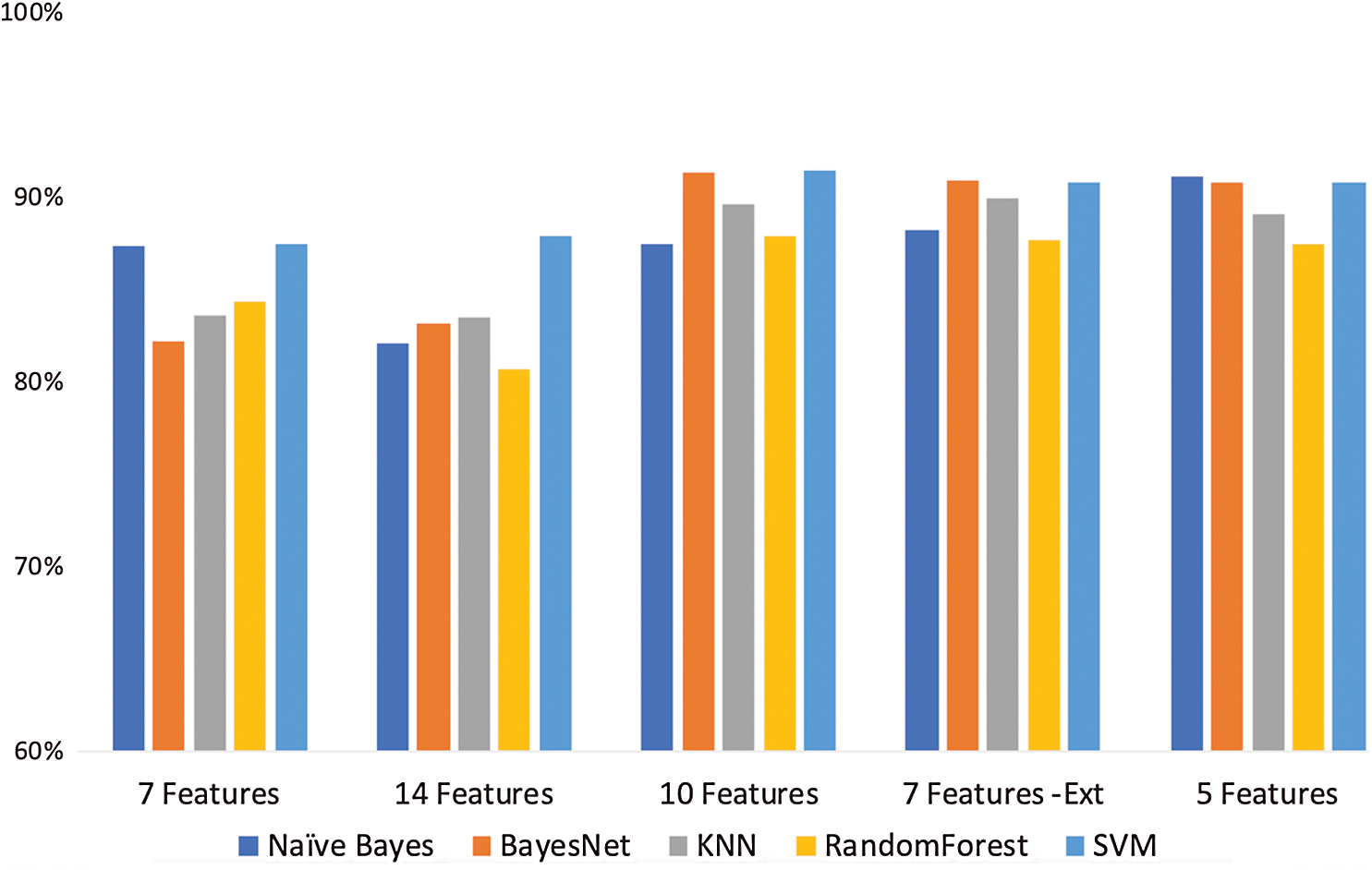
Figure 4: Classifier accuracy rates under various numbers of selected features for classification

In this work, our proposed approach has been studied to detecting APTs relevant for a rather generic IoT framework. Further research may consider applying the Cyber Kill Chain concept to securing specific areas of IoT-enabled applications, such as [46–48].

In this work, we used an APT dataset and reconstructed it to match with the CKC stages. We then performed feature extraction, feature selection, and classification until the final 5 features were selected, as shown in Tab. 3. Overall, we obtained a performance score of 91.1%. We used some of the alerts in multiple stages of the CKC compared to the one to one matching between alerts and stages used by dataset providers. We used feature selection to reduce the impact this would have had on our model’s overall prediction accuracy. We believe it was sensible to use some of the alerts in multiple stages, given this will test the performance of the model more rigorously and the fact that alerts will often appear in multiple stages during the APT attack lifecycle.

The APT dataset we have used is not large, and the original features were only 8, 1 label, and 3676 observations. Relevant cyber-security works would benefit from the incorporation of more detection modules and features. We intend to expand on this research in our future work and plan to build a much larger dataset, which contains the detection modules proposed in our work, as shown in Fig. 3.

Funding Statement: The work of Y. Ahmed and A. T. Asyhari was supported in part by the School of Computing and Digital Technology at Birmingham City University. The work of M. A. Rahman was supported in part by the Flagship Grant RDU190374.

Conflicts of Interest: The author(s) declare that they have no conflict of interest to report regarding the present study.

References

I. Ponemon. (2020). “Cost of a data breach report,” IBM Technical Report.
A. Ahmad, J. Webb, K. C. Desouza and J. Boorman. (2019). “Strategically-motivated advanced persistent threat: Definition, process, tactics and a disinformation model of counterattack,” Computers & Security, vol. 86, pp. 402–418.
J. Kutscher. (2020). “M-Trends 2020: Insights from the front lines,” Milpitas, CA, USA, . [Online]. Available: https://www.fireeye.com/blog/threat-research/2020/02/mtrends-2020-insights-from-the-front-lines.html [Accessed: September 03, 2020].
Centrify. (2020). “Remote working has increased the risk of a cyber breach, says three quarters of UK businesses,” Santa Clara, CA, USA, . [Online]. Available: https://www.centrify.com/about-us/news/press-releases/2020/remote-working-increased-risk-cyber-breach/ [Accessed: September 03, 2020].
Verizon. (2020). “Data breach investigation report,” Verizon Technical Report.
Malwarebytes. (2020). “APTs and Covid-19: How advanced persistent threats use the Coronavirus as a lure,” Malwarebytes Technical Report.
GReAT. (2020). “APT trends report Q1 2020 APT trends report Q1 2020,” SECURELIST, Kaspersky, . [Online]. Available: https://securelist.com/apt-trends-report-q1-2020/96826/ [Accessed: September 03, 2020].
Security Magazine. (2020). “Coronavirus campaign spreading Malware,” Troy, MI, USA: BNP Media, . [Online]. Available: https://www.securitymagazine.com/articles/91646-coronavirus-campaigns-spreading-malware [Accessed: September 03, 2020].
I. Ghafir, M. Hammoudeh, V. Prenosil, L. Han, R. Hegarty et al. (2018). , “Detection of advanced persistent threat using machine-learning correlation analysis,” Future Generation Computer Systems, vol. 89, pp. 349–35
FireEye. (2020). “FireEye ecosystem: Survival in cyberspace isn’t easy,” FireEye, Milpitas, CA, USA, . [Online]. Available: https://www.fireeye.com [Accessed: September 03, 2020].
Kaspersky. (2020). “Kaspersky APT intelligence reporting,” Kaspersky, Moscow, Russia, . [Online]. Available: https://www.kaspersky.com/enterprise-security/apt-intelligence-reporting [Accessed: September 03, 2020].
FireEye. (2020). “Double Dragon: APT41, a dual espionage and cyber crime operation,” FireEye, Milpitas, CA, USA, . [Online]. Available: https://content.fireeye.com/apt-41/rpt-apt41/ [Accessed: September 03, 2020].
A. Alshamrani, S. Myneni, A. Chowdhary and D. Huang. (2019). “A survey on advanced persistent threats: Techniques, solutions, challenges, and research opportunities,” IEEE Communications Surveys & Tutorials, vol. 21, no. 2, pp. 1851–1877.
A. Lemay, J. Calvet, F. Menet and J. M. Fernandez. (2018). “Survey of publicly available reports on advanced persistent threat actors,” Computers & Security, vol. 72, pp. 26–59.
M. Li, W. Huang, Y. Wang, W. Fan and J. Li. (2016). “The study of APT attack stage model,” in Proc. IEEE/ACIS 15th Int. Conf. on Computer and Information Science, Okayama, Japan, pp. 1–5.
T. Yadav and A. M. Rao. (2015). “Technical aspects of cyber kill chain,” in Proc. Int. Symp. on Security in Computing and Communications, Kochi, India, pp. 438–452.
D. Kiwia, A. Dehghantanha, K.-K. R. Choo and J. Slaughter. (2018). “A cyber kill chain based taxonomy of banking Trojans for evolutionary computational intelligence,” Journal of Computational Science, vol. 27, pp. 394–409.
P. N. Bahrami, A. Dehghantanha, T. Dargahi, R. M. Parizi, K.-K. R. Choo et al. (2019). , “Cyber kill chain-based taxonomy of advanced persistent threat actors: Analogy of tactics, techniques, and procedures,” Journal of Information Processing Systems, vol. 15, no. 4, pp. 865–889.
S. Siddiqui, M. S. Khan, K. Ferens and W. Kinsner. (2016). “Detecting advanced persistent threats using fractal dimension based machine learning classification,” in Proc. ACM Int. Workshop on Security and Privacy Analytics, New Orleans, Louisiana, USA, pp. 64–69.
W.-L. Chu, C.-J. Lin and K.-N. Chang. (2019). “Detection and classification of advanced persistent threats and attacks using the support vector machine,” Applied Sciences, vol. 9, no. 21.
R. Brewer. (2014). “Advanced persistent threats: Minimizing the damage,” Network Security, vol. 2014, no. 4, pp. 5–9.
P. Giura and W. Wang. (2012). “A context-based detection framework for advanced persistent threats,” in Proc. Int. Conf. on Cyber Security, Washington, DC, USA, pp. 69–74.
F. A. Garba, S. B. Junaidu, I. Ahmad and M. Tekanyi. (2019). “Proposed framework for effective detection and prediction of advanced persistent threats based on the cyber kill chain,” Scientific & Practical Cyber Security Journal, vol. 3, pp. 1–11.
VERIS. (2020). “The vocabulary for event recording and incident sharing,” VERIS Community, . [Online]. Available: http://veriscommunity.net/index.html [Accessed: September 03. 2020].
B. Anderson and D. McGrew. (2017). “OS fingerprinting: New techniques and a study of information gain and obfuscation,” in Proc. IEEE Conf. on Communications and Network Security, Las Vegas.
The Register. (2015). “Robots.txt tells hackers the places you don’t want them to look,” . [Online]. Available: https://www.theregister.com/2015/05/19/robotstxt/ [Accessed: September 03, 2020].
S. Marchal, J. Francois, C. Wagner and T. Engel. (2012). “Semantic exploration of DNS,” in Proc. Int. Conf. on Research in Networking, Prague, Czech Republic, pp. 370–384.
A. Shulman, M. Cherny and S. Dulce. (2015). “Compromised insider honey pots using reverse honey tokens,” US Patent US20150135266A1.
N. Nissim, R. Yahalom and Y. Elovici. (2017). “USB-based attacks,” Computers & Security, vol. 70, pp. 675–688.
J. P. Farwell and R. Rohozinski. (2011). “Stuxnet and the future of cyber war,” Survival, vol. 53, pp. 23–40.
F. Vanhoenshoven, G. Napoles, R. Falcon, K. Vanhoof and M. Koppen. (2016). “Detecting malicious URLs using machine learning techniques,” in Proc. IEEE Symp. Series on Computational Intelligence, Athens, Greece, pp. 1–8.
S. Gupta and B. B. Gupta. (2017). “Cross-site scripting (XSS) attacks and defense mechanisms: Classification and state-of-the-art,” International Journal of System Assurance Engineering and Management, vol. 8, pp. 512–530.
D. Hendler, S. Kels and A. Rubin. (2018). “Detecting malicious powershell commands using deep neural networks,” in Proc. Asia Conf. on Computer and Communications Security, Incheon, Korea, pp. 187–197.
O. Thonnard, L. Bilge, G. O’Gorman, S. Kiernan and M. Lee. (2012). “Industrial espionage and targeted attacks: Understanding the characteristics of an escalating threat,” in Proc. Int. Workshop on Recent Advances in Intrusion Detection, Amsterdam, The Netherlands, pp. 64–85.
A. Nadler, A. Aminov and A. Shabtai. (2019). “Detection of malicious and low throughput data exfiltration over the DNS protocol,” Computers & Security, vol. 80, pp. 36–53.
O. Al-Jarrah and A. Arafat. (2014). “Network intrusion detection system using attack behavior classification,” in Proc. Int. Conf. on Information and Communication Systems, Irbid, Jordan, pp. 1–6.
M. S. Reza and J. Ma. (2016). “ICA and PCA integrated feature extraction for classification,” in Proc. IEEE Int. Conf. on Signal Processing, Chengdu, China, pp. 1083–1088.
I. T. Jolliffe and J. Cadima. (2016). “Principal component analysis: A review and recent developments,” Philosophical Transactions of the Royal Society A: Mathematical, Physical and Engineering Sciences, vol. 374, no. 2065, pp. 20150202.
F. Husson and J. Josse. (2014). “Multiple correspondence analysis,” Visualization and Verbalization of Data, pp. 165–184.
H. Abdi, L. J. Williams and D. Valentin. (2013). “Multiple factor analysis: Principal component analysis for multitable and multiblock data sets,” Wiley Interdisciplinary Reviews: Computational Statistics, vol. 5, no. 2, pp. 149–179.
J. Li, K. Cheng, S. Wang, F. Morstatter, R. P. Trevino et al. (2017). , “Feature selection: A data perspective,” ACM Computing Surveys, vol. 50, no. 6, pp. 1–45.
M. N. Murthy and V. S. Devi. (2011). Pattern Recognition: An Algorithmic Approach. London: Springer-Verlag.
J. Cheng and R. Greiner. (1999). “Comparing Bayesian network classifiers,” in Proc. Conf. on Uncertainty in Artificial Intelligence, Stockholm, Sweden, pp. 101–108.
D. Stabili, M. Marchetti and M. Colajanni. (2017). “Detecting attacks to internal vehicle networks through Hamming distance,” in Proc. AEIT Int. Annual Conf., Cagliari, Italy, pp. 1–6.
S. J. Lee, P. D. Yoo, A. T. Asyhari, Y. Jhi, L. Chermak et al. (2020). , “IMPACT: Impersonation attack detection via edge computing using deep autoencoder and feature abstraction,” IEEE Access, vol. 8, pp. 65520–65529.
M. A. Rahman, M. N. Kabir, S. Azad and J. Ali. (2015). “On mitigating hop-to-hop congestion problem in IoT enabled intra-vehicular communication,” in Proc. Int. Conf. on Software Engineering and Computer Systems, Malaysia, pp. 213–217.
M. A. Rahman and A. T. Asyhari. (2019). “The emergence of Internet of Things (IoTConnecting anything, anywhere,” Computers, vol. 8, no. 2, pp. 213–217.
M. A. Rahman, M. M. Hasan, A. T. Asyhari and M. Z. A. Bhuiyan. (2017). “A 3D-collaborative wireless network: Towards resilient communication for rescuing flood victims,” in Proc. IEEE 15th Int. Conf. on Dependable, Autonomic and Secure Computing, USA, pp. 385–390.

Computers, Materials & Continua DOI:10.32604/cmc.2021.014223
Article