DOI:10.32604/cmc.2021.014507
| Computers, Materials & Continua DOI:10.32604/cmc.2021.014507 | |
| Article |
A Computational Analysis to Burgers Huxley Equation
1Department of Mathematics, Numl University, Islamabad, 44000, Pakistan
2Department of Mathematics, Air University, Islamabad, 44000, Pakistan
3Department of Mathematics, Air University, Multan Campus, Multan, 66000, Pakistan
4Department of Mathematics, King Abdulaziz University, Jeddah, Saudi Arabia
*Corresponding Author: Muhammad Shoaib Arif. Email: shoaib.arif@mail.au.edu.pk
Received: 24 September 2020; Accepted: 04 December 2020
Abstract: The efficiency of solving computationally partial differential equations can be profoundly highlighted by the creation of precise, higher-order compact numerical scheme that results in truly outstanding accuracy at a given cost. The objective of this article is to develop a highly accurate novel algorithm for two dimensional non-linear Burgers Huxley (BH) equations. The proposed compact numerical scheme is found to be free of superiors approximate oscillations across discontinuities, and in a smooth flow region, it efficiently obtained a high-order accuracy. In particular, two classes of higher-order compact finite difference schemes are taken into account and compared based on their computational economy. The stability and accuracy show that the schemes are unconditionally stable and accurate up to a two-order in time and to six-order in space. Moreover, algorithms and data tables illustrate the scheme efficiency and decisiveness for solving such non-linear coupled system. Efficiency is scaled in terms of L2 and  norms, which validate the approximated results with the corresponding analytical solution. The investigation of the stability requirements of the implicit method applied in the algorithm was carried out. Reasonable agreement was constructed under indistinguishable computational conditions. The proposed methods can be implemented for real-world problems, originating in engineering and science.
Keywords: Burgers Huxley equation; finite difference schemes; HOC schemes; Thomas algorithm; Von-Neumann stability analysis
This paper describes the multiplex schemes solution for two dimensional non-linear Burgers Huxley equation. Such an equation serves as the coupling between the  diffusive terms and Z(Zx + Zy) the convectional phenomena. This equation is of high importance for showing a prototype model describing the interaction between reaction mechanisms, convection effects and diffusion transports. It is the combination of both Burgers & Huxley phenomena with non-linear term means reactions kind of characteristics behaviour, to capture some features of fluid turbulence which caused by the effects of convection & diffusion [1–3]. It is a quantitative paradigm which deals with the flow of electric current through the surface membrane of a giant nerve fibre. Nerve pulse propagation in nerve fibres and wall motion in liquid crystals. Recently research has been measured to investigate two dimensional Burgers Huxley phenomena for understanding the various physical flows in fluid theory [4–6] which leads to implementing a novel methodology for studying new insights [7,8]. It is worth mentioning that there is a vast amount of different approaches available in the literature to calculate the solutions of non-linear systems of partial differential equations. Seeking the Burgers Huxley equations numerical solution, wavelet collocation methods for the solution of Burgers Huxley equations [9] have already been studied in combination with variational iteration technique [10,11]. Moreover, the propagation of genes (Burger & Fisher) and Reaction-Diffusion (Gray Scott) models [12,13] investigated largely by the technique of computation [14]. On the other hand, optimal homotopy asymptotic & homotopy perturbation method was carried out to find the approximate solution of Boussinesq-Burgers equations [15]. Finally, some novel techniques also take into account like chaos theory [16], non-linear optics and fermentation process [17,18]. Wazwaz obtained the solitary wave solutions of one dimensional Burgers Huxley equation using tanh-coth method [19]. Hashim et al. [20,21] using Adomian Decomposition Method. Molabahrami et al. [22] used the homotopy analysis method to find the solution of one dimensional Burger Huxley equation also Efimova et al. [23] find the travelling wave solution of such equation. Batiha et al. [24] used Hope-Cole transformation with Gao et al. [25] find the exact solution of the generalized Burgers equation.
This research aims to deal with higher-order compact schemes with the finite difference methodology [8]. Our primary focus is to attain a compatible scheme which is highly efficient and easy to implement with better accuracy. Although, Burgers Huxley equation can be in three dimensions still some features kept unexplored in the two-dimensional scenario. Let us explorer some new insights in BH equation which consists of the two-dimensional domain which can be written as:

where 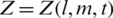 is the unknown velocity &
  . Laplacian can be defined as

with two dimensional behavior,

also  is a non-linear reaction term. The coefficient
  are advection and reactions coefficients accordingly with
  &
&  . These parameters describe the interaction between reaction mechanisms, convection effects & diffusion transports [26,27]. Let us consider the initial condition,

which can be seen from the upcoming Eq. (12). The Dirichlet boundary conditions are given by,

where  is a rectangular domain in R2 &
  are given sufficiently smooth functions, and
  may represent unknown velocity, whereas
  represents convection terms along with linear diffusion
  . Such phenomena perpetuate the ionic mechanisms underlying the initiation and propagation of action potentials in the squid giant axon [28,29].
More generally, it is a challenging task for determining and preservation of physical properties like accuracy, stability, convergence criteria and design efficiency for the given two-dimensional problem. This equation can be an effective procedure for the solution of various deterministic problems in physics, biology and chemical reactions. Also, deals in the investigation of the growth of colonies of bacteria consider population densities or sizes, which are non-negative variables. Most non-linear models of real-life problems are still very challenging to solve either numerically or theoretically. There has recently been much attention devoted to the search for better and more efficient solution methods for determining a solution, analytical or numerical, to non-linear models [30,31]. In [31–34] authors present a method used to solve partial equations with the use of artificial neural networks and an adaptive strategy to collocate them. To get the approximate solution of the partial differential equations Deep Neural Networks (DNNs) has been used, which shows impressive results in areas such as visual recognition [35]. Recently in [36], authors develop a numerical method with third-order temporal accuracy to solve time-dependent parabolic and first-order hyperbolic partial differential equations. We focused on elaborating further by comparing analytical and numerical techniques.
The dynamical balance between the non-linear reaction term and diffusive effects which constitute stable waveform after colliding with each other. In (1) the negative coefficients of  and Z3 follow the physical behaviour of two dimensional BH Eq. (1). Such an equation can be converted into the non-linear ordinary differential equation which is as follows:

Let  , the wave variable which balances the non-linear reaction term (
 ) where
  are index values and diffusion transport (the highest derivative involved), we have
  . This enables us to set: Put M = 1 in (6) we get

Let  , and
, and 

Substitutes aforementioned in Eq. (6), we have the following solution to (7)

Arranging the coefficients of  , and equating these coefficients to zero, the system of algebraic equations in
  and e are obtained. By solving the following set of the algebraic system of equations, we have the following form:

In Eq. (10), the solution is of the form:
Case 1: We found that b1 = 0,
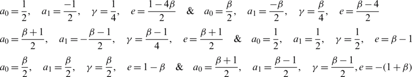
Case 2: We found that a1 = 0,

From Cases 1 and 2, the kink solution is of the form:
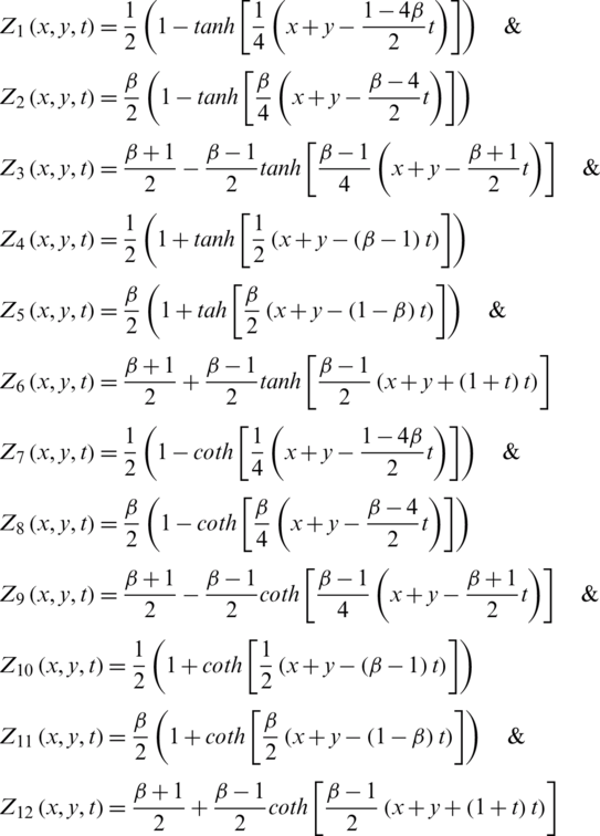
Now by solving (1) using the tanh-coth method, the analytical solution (kink solution) is in a compact form in both cases is as follows:

with initial condition:

where Z is the unknown velocity, and  are wavenumbers which are developed during the solution of BH equation.
3 Description of Compact Schemes
Let us discretize the spatial domain which consists of N and M positive integers, such that hl and hm present step sizes along with l and m directions, respectively [37]. The spatial nodes can be denoted by  , namely, li = ihl,
  & mj = jhm,
  . For the temporal domain, let us take dt as time-step discretization,
  , with
  . Also
  with
with  [37–39]. Where
  is the temporal step size. Set
  , for any
  , with some more notations:

for  .
.
Implementation Procedure:
Let us we divide (1) into two parts such as:

Now considering one-dimensional steady convection-diffusion equation in the following form:

where  are the constants while
  are the convective velocities.
  is the smooth functions of l and m may represent the reaction, vorticity. Now the three-point scheme is as follows:

Now applying the Taylor series expansion to Eq. (14) we have the following results:


where 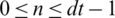 and the truncation error is

By adding Eqs. (17) and (18) we have the following form (1) which yields:

where  ,
, 
Apply Crank–Nicholson time discretization, which leads to:

where  represents the truncation error [36–39]. The existence and uniqueness of the solutions of the scheme (21) can be easily found by positive definite property. By applying operators and simplifying the (21) in compact form, The scheme is a system of linear equations based on variable
  , then after applying operators 21 can be written in the following way:

where  are all constants coefficients of
  and
and  which includes
  and constant values. Let
  …
… where
where  . The matrix form of the compact scheme is as follows

By calculating and simplifying the terms, we have the following tridiagonal matrix if of the form:

where D11 matrix is the same as the matrix D33. The Eq. (23) is a tridiagonal block matrix.

The matrix we have generated is diagonally dominant and can solve through Thomas algorithm. Which authenticate the consistency & accuracy of the solution of the form  .
.
4 Description of Six order Compact Finite Difference Scheme
For complex systems the results will be dependent on the formation of the mesh, We apply higher-order compact scheme at the system in Eq. (1) with a uniform mesh at  . Scheme description is as follows:
Interior Boundary Points:
The compact schemes at interior boundary points are as follows:

Above schemes in Eq. (25) constitute  family of tridiagonal structure with parametric values
  . For
. For  , we get fourth-order accurate scheme while using
  11, the scheme becomes sixth-order accurate which leads to
  [36–39]. Also, near boundary points, we have to construct a sixth-order compact scheme to sustain accuracy throughout the two-dimensional domain [36–39].
First Boundary Point 1:
At the first boundary point, the six order compact scheme is of the following form.

Above system in Eq. (26), the coefficients can be found by matching Taylor’s series expansion comparing with various orders up to order O7, as a result, construction of the linear system is obtained. By constructing the linear system values of d′s, which can be solved in the usual way to get the following along l direction,  [36,37]. Others ones can found in the same way.
2nd Boundary Point 2:

Above system in Eq. (27), by constructing the linear system values of d′s, which can be solved in the usual way to get the following along l direction,  [36–39]. Others ones can found in the same way.
Nth Boundary Point:
At Nth boundary point of six order compact scheme is of the following way:

Above system in Eq. (28), by constructing the linear system values of d′s, which can be solved in the usual way as done in boundary point 1 and 2.
Implementation Algorithm:
By arranging Eqs. (26)–(28) in the following algorithm:

where P are mentioned in Eq. (1), also matrices A and B are  sparse with triangular nature along C and D are
  sparse with triangular in shape.
Theorem:
The truncation error in the compact six order finite difference scheme for equations in the system (1) is,

The convergence benchmark, efficiency and accuracy of the proposed scheme in terms of norms can be defined as:


where  denoted as an analytical solution while
  represents the numerical solution by mesh points (
 ). In this experiment
  , where
  is an eigenvalue of
  respectively.
The stability is concerned with the growth or decay of the error produced in the finite-difference solution. For the representation of theoretical analysis, we set P = 0 in Eq. (1). Assuming the boundary conditions are accurately propagating, we can apply the Fourier analysis method to our proposed equation.
 For a time-dependent PDE, the corresponding difference scheme is stable in the norm
  if there exists a constant M such that

where M is independent of  and initial condition e0.
Following the Von Neumann stability analysis criteria, fix the non-linear terms so that for linear stability, the numerical solution can be displayed in the following way:

where  is the amplitude at time level
  is called the imaginary unit.
  leads to wave number in l, and m directions with
  are phase angles. The amplification factor is defined by

By using Eqs. (30) and (35) and dividing by r.h.s of Eq. (35) and simplifying, we have the following form:
where  and Eq. (37) is of the following way:

where R & S are the compact forms of Eq. (37). For stability, it has to satisfy the following condition:

After simplification to an aforementioned condition which holds true. Therefore,  [38–41]. Hence the scheme is unconditionally stable.
The novel numerical scheme is compared with the analytical results of Eq. (1) by using tanh-coth method. For this objective, we consider the same parameter  , and varying
  . Numerical and analytic solutions are compared and justified in term of error norms to magnify the importance of higher accuracy.
Furthermore, to avoid turbulence, by varying  values in the Tab. 1 with grid size
  , dt = 0.001 and grid space =0.3125 with respect to time = 1 is observed. Improvement in accuracy is noted by varying the values of
  parameter. Also, the BH equation produced the best results by using six order compact finite difference scheme. At different
  values, Tab. 2 indicates error which increased at a very low rate by changing the values of
  from high to low which make the comparison to previous work give authentication for accuracy [34]. The truncation error is calculated in Tab. 3, using
  and
and  with fixed grid size
  . By changing time steps dt = 0.001 with the same grid size showed results in the Tab. 4. The approximate results using six order compact scheme correspond to error norm are shown in the Tab. 6. In this, table the comparison of fourth-order and six order are analyzed by refining the temporal space, which shows this scheme is better than the corresponding fourth-order. In the Tab. 7 six order and fourth-order compact finite difference scheme comparison is carried out which measured in term of
  norm. Different parameters are also observed under the same scheme. In the Tab. 8 scheme efficiency encountered using
  , L2 &
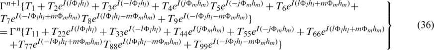
  norms. Graphical representation of numerical schemes on BH equation is observed. Comparison of analytical and numerical results by using fourth and sixth-order compact finite difference scheme has been analyzed. At t = 2,
  , dt = 0.0001,
  can be seen from the Fig. 1. While six order scheme at
  with time-space dt = 0.0001 and grid space
  is seen from the Fig. 2 which shows more accurate and refine results as compared with Fig. 1 using the same parameter. In Figs. 3 and 4, analysis shows that the error norm using fourth-order scheme at
  . While in Fig. 5, we choose
  using a higher-order scheme to analyze error profile at grid size
  . In summary, it is aspirant from the figures and tables; the analytical and numerical solutions are best fitted with generation encrypting. In the end, the novel six order compact scheme is the best agreement with the analytical solution.
Table 1: Fourth-order compact scheme

Table 2: Six order compact scheme


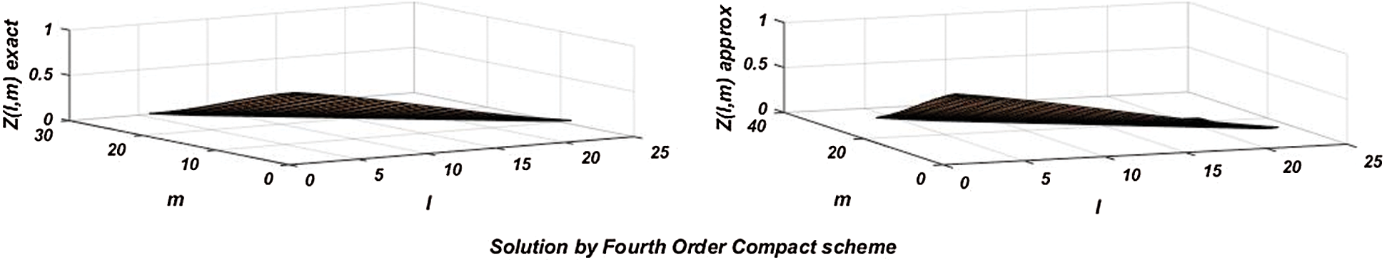
Figure 1: Results obtained by using 4th order scheme at dt = 0.00011 &  at
at 
Figure 2: Results which obtained by using 6th order scheme at dt = 0.0001, &  at a time level 2
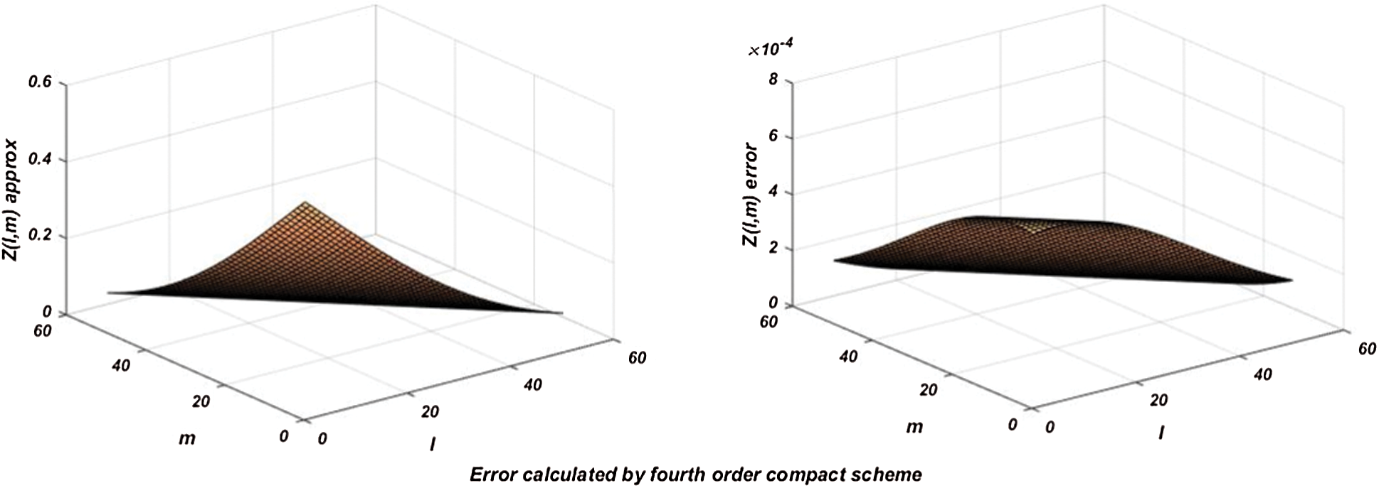
Figure 3: Results for error estimation by using 4th order scheme at dt = 0.001 &  at time 1
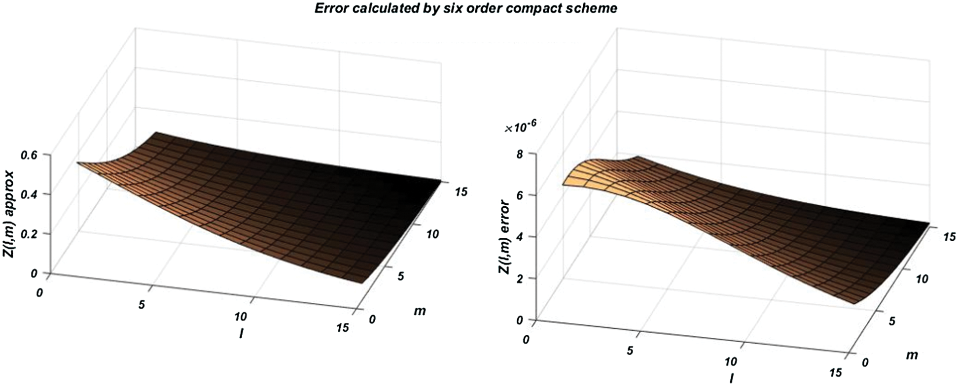
Figure 4: Results for error estimation by using 6th order scheme at dt = 0.001 &  at time 1
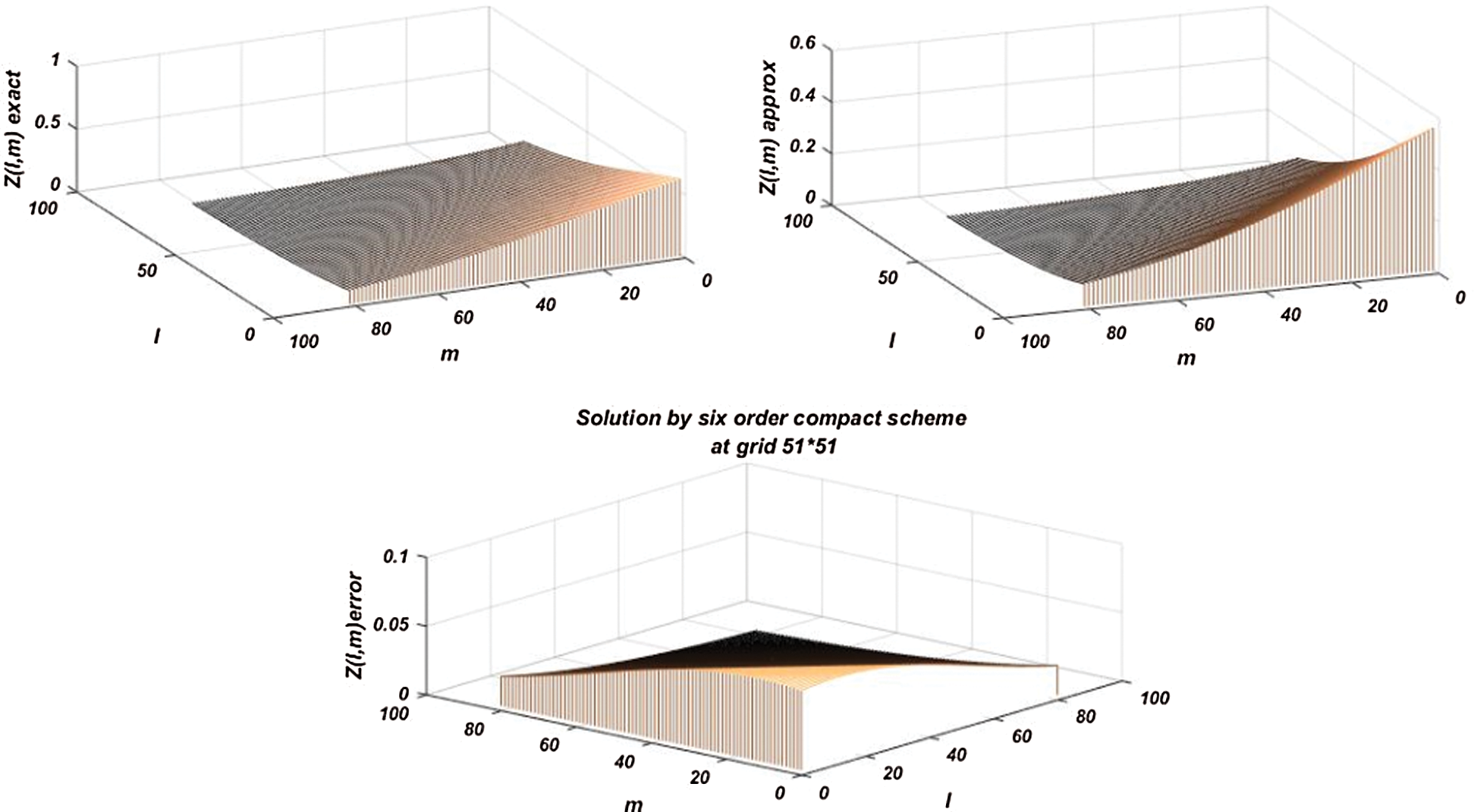
Figure 5: Results obtained by using 6th order scheme at  at time level 0.5
Comparison between approximation and analytical solutions is made at the final time of computation time = 2 s at the critical point  using fourth-order compact scheme at grid size
  .
.
Comparison between approximation and analytical solutions is made at the final time of computation time = 1 at the critical point  using fourth-order compact scheme at grid size
  .
.
Tab. 3 shows error profile data by using fourth-order compact scheme at  for unknown value
  . Self time: is the time spent in a function excluding the time spent in its child functions while
  is the time to execute the algorithm.
Tab. 4 shows error profile data by using Six order compact scheme at  for unknown value
  .
.
Tab. 5 shows a comparison of two schemes at  and
and  for unknowns
  .
.

Tab. 6 shows a comparison of two schemes at  for unknowns
  .
.

6 Central Processing Unit Performance
A combinatorial logic circuit executes the mathematical operation for each function in the algorithm within the central processing unit. To establish the platform of CPU performance along physical memory transmission capacity is observed when the higher-order compact scheme is developed by using MATLAB software [35,39,42,43]. By increasing the grid size, the number of calculations is increased, and it is difficult to overcome such issue which can take a longer time to execute. Because of numerical schemes efficiency, the computational experiment is done on two different computer machines like Lenovo 6th generation having 2.4 GHz 8 cores and 16 GB memory along 5th generation Dell machine having 4 physical cores and 16 logical cores. Different feathers involved in two computational experiments can be analyzed from the following data tables.
Tab. 7 shows results for the different grid using 6th order compact scheme on Lenovo CPU oriented computational machine (MATLAB software).
Table 7: Central processing unit performance

Tab. 8 shows results for the different grid using 6th order compact scheme on DELL CPU oriented computational machine (MATLAB software).
Table 8: Central Processing Unit Performance

To check the relative performance and execution time, here in this algorithm which used two machines, Dell and Lenovo, as follows:

where,

The execution time of the Lenovo machine at  grid size is 170.579 s, and Dell machine execution time at the same grid size is 165.123 s. To calculate the relative performance we have
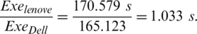
Results conclude that Dell machine is 1.033 faster than the Lenovo machine.
 can be defined as:

where  . For CPU time, the clockrate = 2 GHz, of Lenovo machines and clock rate, is 10 s, by increasing the clockrate means increase
  . The clockrate of Lenovo machine
  . To calculate the clockrate we have
  .2. So

Clock rate performance of Dell machine is, 
Comparison is performed to analyze Dell with Lenovo machines with both clock rate performance and relative performance. Thus MATLAB handles problems with care, and we can analyze results at each point of the loop and any iteration during computations.
Higher-order schemes for determining the two dimensional Burgers Huxley equation was developed in this paper. As it was not studied before by using such schemes of diffusive dissipation of errors. We came to know that the BH equation in two dimensional which is studied to find efficiency, accuracy and stability and by comparing with analytical and numerical approaches in terms of  & relative errors. It is evident from the fact that computed numerical experiments of two dimensional Burgers Huxley equation, solutions obtained by fourth and six order schemes are in good agreement with the analytical solutions. Figures and tables clearly show the tendency of fast and monotonic convergence of the results toward the analytical solution. Also, the computational discretization of the proposed model results in a sparse tridiagonal structure of the matrix, which can be overcome by the Thomas algorithm. Results lead to a remarkable improvement in accuracy, efficiency and computer performance which can be seen from data tables.
Acknowledgement: The authors are thankful to the anonymous referee for their suggestions and helpful comments that improved this article. We are also grateful to Vice-Chancellor, Air University, Islamabad, for providing an excellent research environment and facilities.
Funding Statement: The authors received no specific funding for this study.
Conflicts of Interest: The authors declare that they have no conflicts of interest to report regarding the present study.
1. J. M. Burgers. (1948). “A mathematical model illustrating the theory of turbulence,” Advances in Applied Mechanics, vol. 1, pp. 177–199. [Google Scholar]
2. W. F. Ames. (1995). Finite difference methods for partial differential equations, vol. 22. New York: Academic Press, pp. 1–47. [Google Scholar]
3. J. Noye. (1984). “Finite difference methods for partial differential equations,” North-Holland Mathematics Studies, vol. 83, pp. 95–354. [Google Scholar]
4. J. D. Logan. (2008). An Introduction to Non-Linear Partial Differential Equations. New York: Wily International Science, pp. 1–398. [Google Scholar]
5. G. Sewell. (2005). The Numerical Solution of Ordinary and Partial Differential Equations. Canada: John Wiley and Sons, Inc., Hoboken, New Jersey. [Google Scholar]
6. R. L. Burgen and J. D. Faries. (2011). “Numerical analysis,” in: Book, 9th ed. Brooks/Cole, Cengage Learning. [Google Scholar]
7. N. Taghizadeh, M. Akbari and A. Ghelichzadeh. (2011). “Exact solution of Burgers equations by homotopy perturbation method and reduced differential transformation method,” Australian Journal of Basic and Applied Sciences, vol. 5, pp. 580–589. [Google Scholar]
8. S. S. Ray and A. Gupta. (2013). “On the solution of Burgers–Huxley and Huxley equation using wavelet collocation method,” Computer Modelling in Engineering & Sciences, vol. 91, pp. 409–424. [Google Scholar]
9. J. E. Macas-Daz. (2018). “A modified exponential method that preserves structural properties of the solutions of the Burgers Huxley equation,” International Journal of Computer Mathematics, vol. 95, no. 1, pp. 3–19. [Google Scholar]
10. S. S. Ray and A. Gupta. (2014). “Comparative analysis of variational iteration method and Haar wavelet method for the numerical solutions of Burgers Huxley and Huxley equations,” Journal of Mathematical Chemistry, vol. 52, pp. 1066–1080. [Google Scholar]
11. R. Munafo. (2009). “Reaction diffusion by the Gray-Scott model: Pearsons parameterization,” Unpublished Material, Available: http://mrob.com/pub/comp/xmorphia/index.html, under Creative Commons Attribution Non-Commercial 2.5 License. [Google Scholar]
12. M. Saqib, S. Hasnain and D. Mashat. (2017). “Highly efficient computational methods for two dimensional coupled non-linear unsteady convection-diffusion problems,” IEEE Acess, vol. 5, pp. 7139–7148. [Google Scholar]
13. A. Gupta and S. S. Ray. (2014). “On the solutions of fractional Burgers Fisher and generalized Fisher equations using two reliable methods,” International Journal of Mathematics and Mathematical Sciences, vol. 2014, pp. 1–16. [Google Scholar]
14. A. Gupta and S. S. Ray. (2014). “Comparison between homotopy perturbation method and optimal homotopy asymptotic method for the soliton solutions of Boussinesq Burger equations,” Computer & Fluids, vol. 103, no. 1, pp. 34–41. [Google Scholar]
15. P. Vadasz and S. Olek. (2000). “Convergence and accuracy of Adomian decomposition method for the solution of Lorenz equation,” International Journal of Heat and Mass Transfer, vol. 43, no. 10, pp. 1715–1734. [Google Scholar]
16. H. N. A. Ismail, K. Raslan and A. A. Abd-Rabboh. (2004). “Adomian decomposition method for Burgers–Huxley and Burgers Fisher equations,” Applied Mathematics and Computation, vol. 159, no. 1, pp. 291–301. [Google Scholar]
17. I. Hashim, M. S. M. Noorani and M. R. S. Al-Hadidi. (2006). “Solving the generalized Burgers Huxley equation using the Adomian decomposition method,” Mathematical and Computer Modelling, vol. 43, no. 1, pp. 1404– 1411. [Google Scholar]
18. A. M. Wazwaz. (2008). “Analytic study on Burgers, Fisher, Huxley equations and combined forms of these equations,” Applied Mathematics and Computation, vol. 195, no. 1, pp. 754–761. [Google Scholar]
19. H. N. A. Ismail, K. Raslan and A. A. Abd-Rabboh. (2004). “Adomian decomposition method for Burgers Huxley and Burgers Fisher equations,” Applied Mathematics and Computation, vol. 159, no. 1, pp. 291–301. [Google Scholar]
20. I. Hashim, M. S. M. Noorani and M. R. S. Al-Hadidi. (2006). “Solving the generalized Burgers Huxley equation using the Adomian decomposition method,” Mathematical and Computer Modelling, vol. 43, no. 11–12, pp. 1404–1411. [Google Scholar]
21. I. Hashim, M. S. M. Noorani and B. Batiha. (2006). “A note on the Adomian decomposition method for the generalized Huxley equation,” Applied Mathematics and Computation, vol. 181, no. 2, pp. 1439–1445. [Google Scholar]
22. A. Molabahramia and F. Khani. (2009). “The homotopy analysis method to solve the Burgers Huxley equation,” Nonlinear Analysis: Real World Applications, vol. 10, no. 2, pp. 589–600. [Google Scholar]
23. O. Y. U. Efimova and N. A. Kudryashov. (2004). “Exact solutions of the Burgers Huxley equation,” Journal of Applied Mathematics and Mechanics, vol. 68, no. 3, pp. 413–420. [Google Scholar]
24. B. Batiha, M. S. M. Noorani and I. Hashim. (2008). “Application of variational iteration method to the generalized Burgers Huxley equation,” Chaos Solitons and Fractals, vol. 36, no. 3, pp. 660–663. [Google Scholar]
25. H. Gao and R. X. Zhao. (2010). “New exact solutions to the generalized Burgers–Huxley equation,” Applied Mathematics and Computation, vol. 217, no. 4, pp. 1598–1603. [Google Scholar]
26. R. K. Mohanty, W. Dai and D. Liu. (2015). “Operator compact method of accuracy two in time and four in space for the solution of time-dependent Burgers–Huxley equation,” Numerical Algorithms, vol. 70, no. 3, pp. 591–605. [Google Scholar]
27. M. Ablowitz, B. Fuchssteiner and M. Kruskal. (1987). “Topics in soliton theory and exactly solvable non-linear equations,” in Proc. of the Conf. on Non-linear Evolution Equations, Solitons and the Inverse Scattering Transform, Oberwolfach, Germany, pp. 1–352. [Google Scholar]
28. A. L. Hodgkin and A. F. Huxley. (1952). “A quantitative description of membrane current and its application to conduction and excitation in nerve,” Journal of Physiology, vol. 117, no. 4, pp. 500–554. [Google Scholar]
29. G. Adomian. (1988). “A review of the decomposition method in applied mathematics,” Journal of Mathematical Analysis and Applications, vol. 135, no. 2, pp. 501–544. [Google Scholar]
30. E. Y. Deeba and S. A. Khuri. (1996). “A decomposition method for solving the non-linear Klein–Gordon equation,” Journal of Computational Physics, vol. 124, no. 2, pp. 442–448. [Google Scholar]
31. X. Y. Wang, Z. S. Zhu and Y. K. Lu. (1990). “Solitary wave solutions of the generalized Burgers Huxley equation,” Journal of Physics A: Mathematical and General, vol. 23, no. 3, pp. 271–274. [Google Scholar]
32. A. M. Wazwaz. (2002). Partial Differential Equations, Methods and Applications. The Netherland: Balkema Publishers. [Google Scholar]
33. M. Saqib, S. Hasnain and D. Mashat. (2017). “Computational solutions of three dimensional advection-diffusion equation using fourth-order time-efficient alternating direction implicit scheme,” AIP Advances, vol. 7, pp. 85306. [Google Scholar]
34. J. Jichun and Y. T. Chen. (2020). Computational Partial Differential Equations Using Matlab, 2nd ed. Boca Raton, London, New York: Chapman and Hall/CRC Applied Mathematics and Nonlinear Science Series. [Google Scholar]
35. Y. Huang, M. H. N. Skandari, F. Mohammadizadeh, H. A. Tehrani, S. G. Georgiev et al. (2019). , “Space-time spectral collocation method for solving Burgers equations with the convergence analysis,” Symmetry, vol. 11, no. 12, pp. 1439. [Google Scholar]
36. K. N. Tripathi. (2018). “Analytical solution of two-dimensional non-linear space time-fractional Burgers Huxley equation using fractional sub equation method,” National Academy Science Letters, vol. 41, no. 5, pp. 295–299. [Google Scholar]
37. J. Wei and M. Winter. (2003). “Asymmetric spotty patterns generated by Gray Scott Model in R2,” Studies in Applied Mathematics, vol. 110, no. 1, pp. 63–102. [Google Scholar]
38. K. Zhang, J. C. Wong and R. Zhang. (2008). “Second order implicit and explicit schemes to Gray Scott model,” Journal of Computational and Applied Mathematics, vol. 213, no. 2, pp. 559–581. [Google Scholar]
39. S. A. M. Tonekaboni. (2013). “Mathematical investigation of two-dimensional pattern formation,” International Journal of Biological Research, vol. 2, no. 1, pp. 1–5. [Google Scholar]
40. H. Guo, X. Zhuang and T. Rabczuk. (2019). “A deep collocation method for the bending analysis of Kirchhoff plate,” Computers, Materials & Continua, vol. 59, no. 2, pp. 433–456. [Google Scholar]
41. C. Anitescu, E. Atroshchenko, N. Alajlan and T. Rabczuk. (2019). “Artificial neural network methods for the solution of second-order boundary value problems,” Computers, Materials & Continua, vol. 59, no. 1, pp. 345–359. [Google Scholar]
42. E. Samaniego, C. Anitescu, S. Goswami, V. M. Nguyen-Thanh, H. Guo et al. (2020). , “An energy approach the solution of partial differential equations in computational mechanics via machine learning: Concepts, implementation and applications,” Computer Methods in Applied Mechanics and Engineering, vol. 362, no. 15, pp. 112790. [Google Scholar]
43. Pasha S. A., Nawaz Y., Arif M. S. (2021). “A third-order accurate in time method for boundary layer flow problems,” Applied Numerical Mathematics, vol. 161, no. 1, pp. 13–26. [Google Scholar]
 | This work is licensed under a Creative Commons Attribution 4.0 International License, which permits unrestricted use, distribution, and reproduction in any medium, provided the original work is properly cited. |
 )
) )
)