DOI:10.32604/cmc.2021.012396
| Computers, Materials & Continua DOI:10.32604/cmc.2021.012396 | |
| Article |
Numerical Analysis of Novel Coronavirus (2019-nCov) Pandemic Model with Advection
1Department of Mathematics and Statistics, The University of Lahore, Lahore, Pakistan
2Department of Mathematics, National College of Business Administration and Economics Lahore, Pakistan
3Faculty of Engineering University of Central Punjab Lahore, Pakistan
4Faculty of Mathematics and Statistics, Ton Duc Thang University, Ho Chi Minh City, 72915, Vietnam
5Department of Mathematics, College of Arts and Science at Wadi Aldawaser, Prince Sattam Bin Abdulaziz University, 11991, Alkharj, Kingdom of Saudi Arabia
6Department of Mathematics, University of Management and Technology, Lahore, Pakistan
*Corresponding Author: Ilyas Khan. Email: ilyaskhan@tdtu.edu.vn
Received: 29 June 2020; Accepted: 21 October 2020
Abstract: Recently, the world is facing the terror of the novel corona-virus, termed as COVID-19. Various health institutes and researchers are continuously striving to control this pandemic. In this article, the SEIAR (susceptible, exposed, infected, symptomatically infected, asymptomatically infected and recovered) infection model of COVID-19 with a constant rate of advection is studied for the disease propagation. A simple model of the disease is extended to an advection model by accommodating the advection process and some appropriate parameters in the system. The continuous model is transposed into a discrete numerical model by discretizing the domains, finitely. To analyze the disease dynamics, a structure preserving non-standard finite difference scheme is designed. Two steady states of the continuous system are described i.e., virus free steady state and virus existing steady state. Graphical results show that both the steady states of the numerical design coincide with the fixed points of the continuous SEIAR model. Positivity of the state variables is ensured by applying the M-matrix theory. A result for the positivity property is established. For the proposed numerical design, two different types of the stability are investigated. Nonlinear stability and linear stability for the projected scheme is examined by applying some standard results. Von Neuman stability test is applied to ensure linear stability. The reproductive number is described and its pivotal role in stability analysis is also discussed. Consistency and convergence of the numerical model is also studied. Numerical graphs are presented via computer simulations to prove the worth and efficiency of the quarantine factor is explored graphically, which is helpful in controlling the disease dynamics. In the end, the conclusion of the study is also rendered.
Keywords: 2019-nCov; infectious model with advection; reproductive number; stability analysis; numerical graphs
Novel Coronavirus-19 is a newly emerged virus that initiated from China. Like other viruses, coronavirus needs host cells for replication. It is considered that coronavirus transmitted from bats to humans. This virus out broke in China and was declared a pandemic by WHO, after a short span of time. Zhou et al. [1] developed a mathematical model to study its propagation in China. the virus belongs to the SARS (severe acute respiratory syndrome) family [2]. It affects the nose, upper throat, or lower respiratory tract. The general symptoms of the infection are cough, fever, flu, and shortness of breath. When an infected person coughs or sneezes, its aerosols spread in the environment and when its particles approach a susceptible individual directly or indirectly, the spread of the virus takes place. This process is explained by Kucharski et al. [3]. This virus disseminated rapidly around the globe, including Pakistan [4]. Coronavirus-19 does not have a high rate of mortality even though it is dreadful. As it is a novel virus, no one has immunity against it. Everyone is susceptible to it. So special care and precautionary steps must be followed for safety purposes. There were 22.3 million confirmed COVID-19 cases around the globe. It is the need of the hour to stop the propagation of COVID-19 among the susceptible people. Mathematical modeling plays an important role in predicting the disease dynamics.
Every infectious disease cannot be stopped by applying for the research study and medicines. Many other factors affecting the transmission of the disease should also be taken into consideration [5]. When the mobility of individuals enhances the propagation of the disease then the role of space coordinates as well as time coordinate become influential [6]. In this study, a classical disease model is modified to the advection model by considering the advection terms and some appropriate parameters. By considering these terms, the extended model has become more realistic [7,8]. Jiang et al. [9] investigated the dynamics of coronavirus with clinical signs and symptoms, by using artificial intelligence. Wang et al. [10] studied the constant value problems and arbitrary value problems, moreover, he investigated the numerical solutions to these problems. Tian [11] presented particle swarm optimization with chaos-based initialization for numerical optimization. Naveed et al. [12] investigated the dynamics of the coronavirus model with the delay technique. This model takes into account the dynamics of both the populations i.e., human beings and viruses.
Basic reproductive number R0 is calculated to predict the disease occurrence in the population. The facts show that human behavior can minimize the epidemic level of coronavirus. A compartmental model is used to understand the fundamentals of disease transmission. Currently, the characteristics of the COVID-19 is understood up to a great extent and mathematical models are being presented by many researchers, but the advection process is not considered in these models. Due to this deficiency in the models, clear understanding of the disease dynamics is very difficult. Since, mobility is the basic need of humans to perform numerous activities in daily life. But this essential factor is increasing the virus spread in the community. By considering pros and cons of the COVID-19, we have proposed the mathematical model with advection, which provides us with the understanding of the virus dynamics and its controllability. On the basis of this study, the relevant authorities can formulate the health policy and precautionary measures, with a more feasible approach.
The paper is arranged as follows: in Section 2, the deterministic coronavirus pandemic model and its equilibria are described. Section 3, deals with the numerical method along with its positivity, stability, consistency and convergence analysis. In Section 4, the current work is explained with numerical simulations. Finally, in Section 5, we reach at the conclusion and future direction is also described.
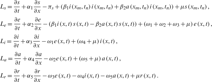
Many researchers took interest in the dynamics of contiguous diseases and their spread with respect to time and space. The compartmental model is used to understand the basics of disease transmission [13]. In the corona epidemic model, advection term is adjusted for the better perception of the disease transmission. The nonstandard FD scheme is constructed with the capability of structure perseverance [14,15]. In this model, the whole population is represented with N(t) and is divided into five compartments as follows: for any time t, the susceptible humans are represented with S(t), exposed humans with E(t), symptomatic infected humans with I(t), asymptomatic infected with A(t) and the recovered humans with R(t). The parameters furnished in the model are described as follows:
 : The recruitment rate
 : The mortality rate with natural incidences or due to virus infection
 : The infection rate of symptomatic humans
 : The infection rate of asymptomatic humans
 : The interaction rate of exposed humans with symptomatic infected humans
 : The interaction rate of exposed humans to asymptomatic infected humans
 : The rate of exposed humans who have recovered from the virus due to natural immunity
 : The rate of symptomatic carriers who have recovered after quarantine
 : The rate of quarantine or isolation of asymptomatic infected humans. In the coronavirus pandemic model following assumption is made that dispersion of virus takes place via symptomatic and asymptomatic carriers who make bilinear incidence rate with the susceptible humans. Without loss of generality, all types of other interactions have been ignored. The flow diagram of the 2019-nCov is presented in Fig. 1 [16]:
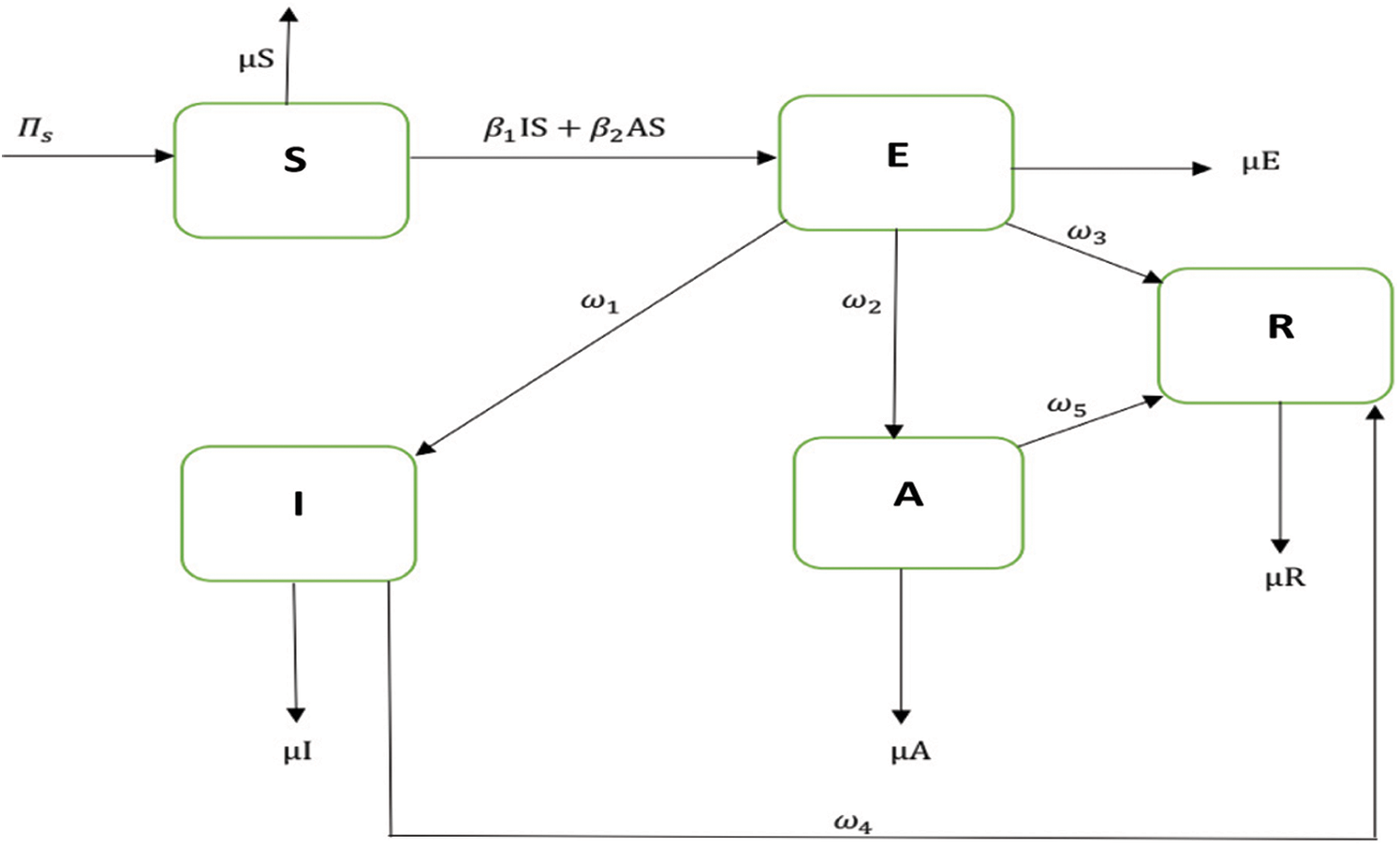
Figure 1: Flow diagram of the model
Azam et al. [17] successfully showed the importance of the advection, representing the bulk transfer of the disease in various compartments of the population. The presented model with the advection terms is a new one and the computations are pretty much connected to physical observations. The SEIAR advective COVID-19 model is described as:


with the initial conditions

and the homogeneous Neumann boundary conditions

The whole population is divided into five compartments as follows: at time  and location
  the susceptible humans are described with S(x, t), exposed humans with E(x, t), symptomatic infected humans with I(x, t), asymptomatic infected with A(x, t) and recovered humans are expressed with R(x, t). Also,
  are positive advection coefficients according to susceptible, exposed, symptomatic infected, asymptomatic infected and recovered classes. The rest of constants are mentioned above in the dynamical model formulation. All the parameters used in PDE’s model are positive.
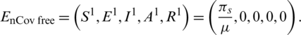
The Eqs. (1) to (5) admit two equilibrium states in the feasible region. The 2019-nCov free equilibrium of the Eqs. (1) to (5) is described as follows:
Also, 2019-nCov existing equilibrium of the system, from Eqs. (1) to (5) is as follows:

where, 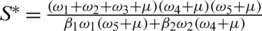 ,
,  ,
,  ,
,  and
and 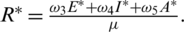
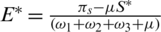
Notice that the reproduction number of the model is defined as  .
.
2.2 Sensitivity Analysis of the Reproduction Number
To test the sensitivity of the reproduction number for each of its parameters, we proceed as follows:
Notice that the parameters like  ,
,  and
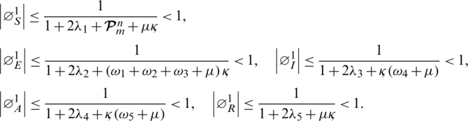
and  are sensitive due to the nature of the model. On the other hand, the rest of the parameters are insensitive. More precisely, the sensitive parameters of the model have a direct relation with the reproduction number. It means that dynamics of the model depends on sensitive parameters i.e. any increase in sensitive parameters will eventually lead to the fact that the virus is existing in the population and vice versa.
By rewriting Eqs. (1) to (5) as


For all  0, the initial conditions will be

And the homogeneous Neumann boundary conditions will be

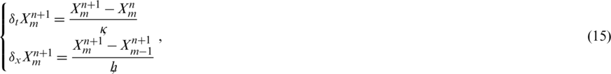
Our proposed scheme is developed by replacing the following time and space partial derivatives in Eqs. (8) to (12),
where  and
and  are partition norms of fixed partitions of intervals [0, T] and [0, L] respectively. Where
  and
and 


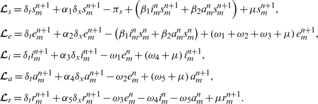
3.1 Development of the Proposed Nonstandard Finite Difference Scheme
Take Eq. (16) and apply discrete forms with respect to time and space respectively as defined in Eq. (15). Then
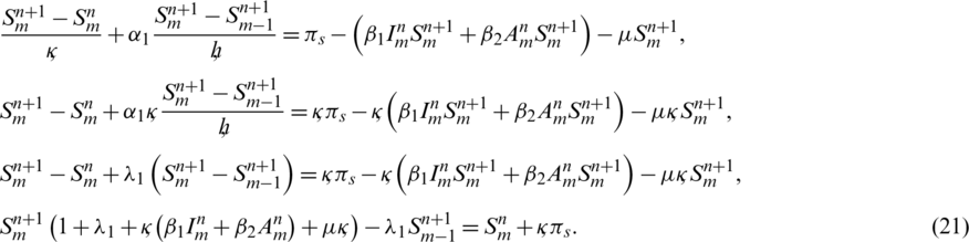
Similarly, by applying same algebraic calculations we can also express Eqs. (17) to (20) in the form of linear equations as follows,


For simplification it is assumed that  ,
,  ,
,  ,
,  and
and  , subject to the following initial and boundary conditions
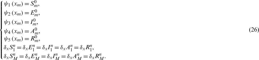
The notations,  are numerical approximations of S, E, I, A, R at point
3.2 M-matrix Theory and Positivity
Our proposed method can also be written in vector form as
For each 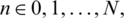


If M represents any of  then these all are real matrices of size (N + 1) * (N + 1). In general M can be written as
The diagonal entries are  ,
,  ,
,  ,
,  and
and  . The negative off-diagonal entries of these matrices are
Here, we will use M-matrix theory to show the positivity of our proposed method. M-matrix is a non-singular square matrix with positive inverse matrix. It is mentionable that diagonal elements are positive and off-diagonals elements are zeros or negative. This fact is of great use to show that our proposed scheme is positivity preserving. i.e., we will use the fact that Q, U, V, W, X are M-matrices and their inverses are non-negative due to restrictions on initial conditions.
Theorem 1: If  are positive functions then our proposed scheme from Eqs. (21) to (25) subject to all the initial and boundary conditions in Eq. (26) are positive then the system is solvable and has positive solutions.
Proof: We will use mathematical induction to prove the positivity and uniqueness. Our initial data guarantees that S0, E0, I0, A0, R0 are all positive vectors.
Let us assume that it is true for some n, i.e., Sn, En, In, An, Rn are positive vectors.
Now, we have to show that it is also true for n + 1. Since Q, U, V, W, X are M-matrices, so the fact that they are non-singular and their inverses exist and they are positive is assured. Furthermore, vectors on the right hand sides of the equations from Eqs. (27) to (31) are also positive.
We can rewrite the system from Eqs. (27) to (31) as follows:
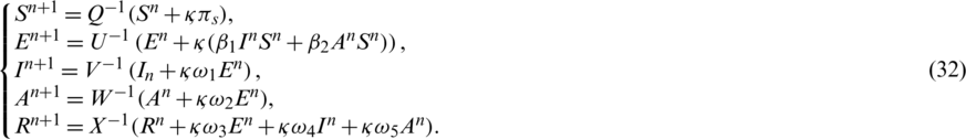
Notice that left hand sides of Eq. (32) are positive. So, it is true for all n. Hence, our proposed scheme is capable of preserving positivity.
Next, we will use discrete form of Gronwall’s inequality. The inequality is stated in the form of following lemma.
Lemma 1: If a discrete function  satisfies the inequality
then  Where
Where  and C6 are positive constants. For the following results, we will assume that numerical solutions of our proposed scheme are uniformly bounded and there exists a common bound
  at point
  for the norms of the numerical solutions obtained from Eqs. (16) to (20).
To establish the non-linear stability of the method, we will consider two numerical solutions 
 of Eqs. (16) to (20) with respective sets of initial data (
 ) and
) and 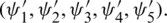


Subject to
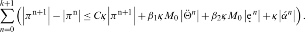
Subtract Eqs. (33) to (37) from Eqs. (16) to (20) simultaneously and let


taking the absolute values on both sides of the last equation and apply triangular inequality as well as using the upper bound M0 on the left-hand side to obtain,
where as  , by taking sum on both sides, we have
using the telescopic sum on left-hand side and then rearranging the terms algebraically, we have
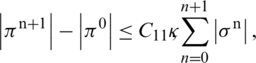
where


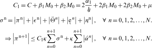
Similarly, we can use telescopic sum for equations Eqs. (35) to (38) and by adopting the same process, following results hold:
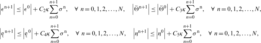
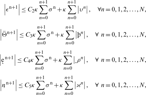
In the above inequalities, the constants C2, C3, C4 and C5 are described as follows:
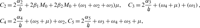
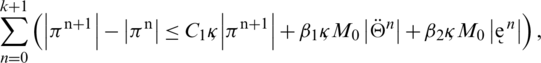
By adding the above inequalities,  , we get,
 , where C6 is given by where
It is clear that C6 is positive and depends upon  .
.
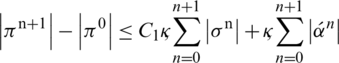
Subtracting  from both sides of the above inequality, we get
This implies that 
It satisfies the condition of Lemma (1). Hence the conclusion followed from lemma 1 that our proposed scheme possesses non-linear stability.
At this stage, we will use von-Neumann criteria to show the linear stability of the proposed method in the result:
Theorem 2: The proposed scheme is linearly stable if  and
and  are positive functions.
Proof: By following von-Neumann criteria let  and
and  be positive numbers and let
  be real numbers. By taking a solution of the proposed discrete model in the form as mentioned in the next step:

next, freeze nonlinear term and put  as a positive constant. After simplification, we have

By applying similar process on rest of the equations, we will get the following


Taking the norm on both sides of Eqs. (53) to (57) and bounding them from above implies that
All these equations satisfy von-Neumann stability criteria. Hence our proposed scheme is stable.
To deal with the consistency analysis of the numerical scheme for Eqs. (16) to (20), let us assume continuous operators as
Let the discrete operators are
Theorem 3: If  and the norm
  then there exists a constant
  independent of
  and
and  such that for each
  ,
,  ,
, 
Proof: Using the boundedness and smoothness of s and applying Taylor’s series, there exist positive constants d1, d2, d3, d4 and d5 such that
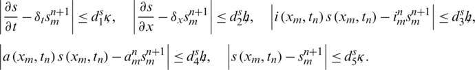
since d1, d2, d3, d4 and d5are independent of  and
and 
As a result  holds if
 , independent of
  and
and 
In a similar fashion, there exist constants  which don’t depend on
  and
and  i.e.,
i.e.,

Hence our proposed scheme is consistent and first order accurate in time and space. Finally, we have the positive constant Åindependent of time and space norms such that

which also doesn’t depend upon norms.
Theorem 4: Let us assume that  ,
,  and
and  be the exact solutions of Eqs. (1) to (5) subject to initial and boundary conditions Eqs. (6) to (7). Then the numerical solutions
  , of Eqs. (16) to (20) subject to Eq. (26) with linear order in time and space converges to exact solution if
  where C > 0.
Proof: For convenience, let us assume that all the constants are the same as mentioned in nonlinear stability. Also, notice that the solutions exist and are positive as discussed earlier in this manuscript. Under these circumstances, it is obvious that the following discrete system is satisfied,


where,  ,
,  and
and  are the local truncation errors.
Since, by using Theorem 3, there exists a constant  independent of norms
  and
and  , such that
 ,
,  ,
,  ,
,  and
and  for each
  .
.
Now subtract Eq. (52) from Eq. (16), we get the following expressions,

let us assume that  ,
,  ,
,  ,
,  ,
,  , after simplifying, we have,
Taking absolute values on both sides of the last equation and applying triangular inequality then use upper bound M0 on the left-hand side to obtain,
where 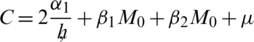 , by taking sum on both sides, we have the following expression:
Using telescopic sum on the left-hand side and then rearranging terms algebraically we have
Since, initial conditions provide that 
Similarly, we can show that
By adding all these inequalities, we have the following:

where 
Then Lemma 
Hence we concluded that
 Our proposed scheme has the convergence of linear order in time and space.
4 Numerical Application and Simulations
The numerical solutions of Eqs. (1) to (5) are in good agreement with the dynamical behavior of the model by using different assumed values of the parameters. Khan et al. [18] presented the parameter values as follows:
 ,
,  ,
,  ,
,  ,
,  ,
,  ,
,  ,
,  ,
,  , for RnCov < 1. For RnCov > 1,
  ,
,  ,
,  ,
,  ,
,  ,
,  ,
,  ,
,  and
and  .
.
The initial conditions are,


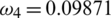
Example 1: nCov free equilibrium ( )
)
For the simulations, we let  ,
,  ,
,  ,
,  ,
,  ,
,  ,
,  ,
,  and
and  . By using initial conditions and performing simple calculations, we get RnCov = 0.7223 < 1.
 is a nCov free equilibrium of the system Eqs. (8) to (12).
Figure 2: Mesh graphs of Eqs. (8) to (12) for different parameters for instance  .5,
.5,  .05,
.05,  .05,
.05,  .5,
.5,  .47876,
  .000398,
  .0854302,
  .09871 and
  .1243, by using initial conditions and RnCov = 0.7223 < 1
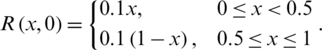
Figure 3: Mesh graphs of Eqs. (8) to (12) for different parameters like  ,
,  ,
,  ,
,  ,
,  ,
,  ,
,  ,
,  and
and  , by using the initial conditions and RnCov = 1.1659 > 1
We use proposed NS finite difference scheme to plot the graphs of Fig. 1. The graphs are approximate solutions of SEIAR system from Eqs. (8) to (12). It can be observed that our proposed scheme is converging to  .
.
Example 2: nCov present equilibrium ( )
)
For the simulations, we fix the parameter values as  ,
,  ,
,  ,
,  ,
,  ,
,  ,
,  ,
,  and
and  . Then RnCov = 1.1659 > 1. We use the proposed NS finite difference scheme from Eqs. (8) to (12) to plot the graphs of Fig. 2. These graphs are the approximate solutions of our discrete system at nCov present equilibrium point. From Fig. 3 we can see that our proposed scheme converges to
  . Furthermore simulations in Fig. 4 show that if we increase the quarantine parameter (a)
  , (b)
, (b)  and (c)
  then this can help us in decreasing the infection in the population.
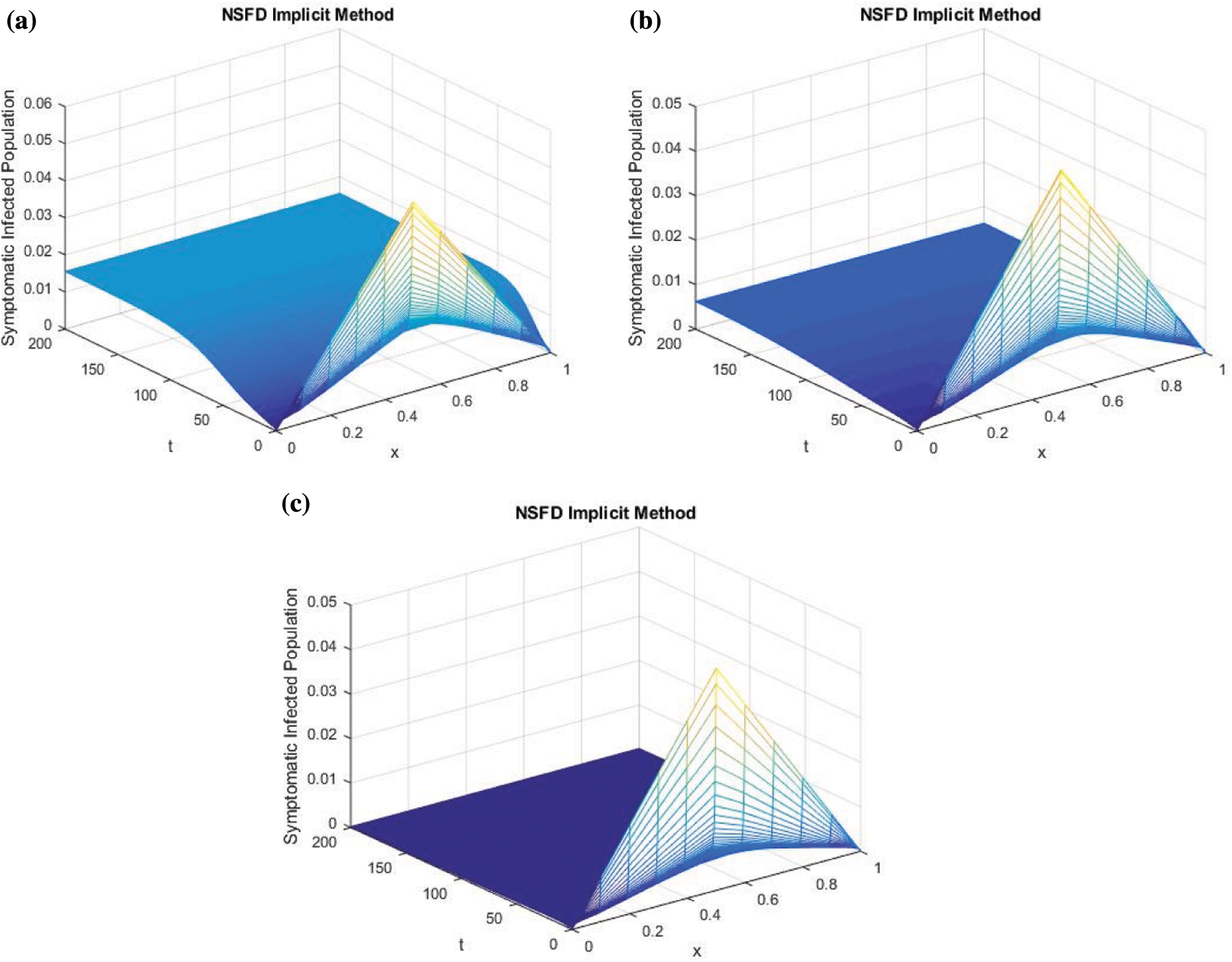
Figure 4: Effect of quarantine strategy on symptomatic infected human by increasing quarantine parameter (a)  , (b)
, (b)  and (c)
From Fig. 4, it is observed that by the implementation of the quarantine strategy the infection can be decreased in the population.
In Fig. 5, we have presented the effect of quarantine on the dynamical behavior of asymptomatic infected compartment of the model. We observe that the increase in quarantine strategy reduce the number of asymptomatic humans.
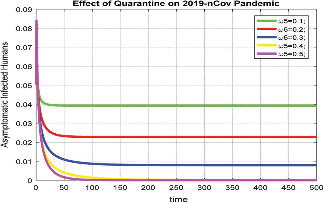
Figure 5: Effect of quarantine
In this article, we have presented the mathematical model and the dynamics of coronavirus (nCov-19). Our new formation deals with the nCov-19 virus transmission. The role of advection in the virus propagation is elaborated. We have investigated the approximate solutions of the proposed PDE model based on logical background and numerical simulations by focusing on the relationship of different biological, environmental and physical factors that determine the spatial spreading of nCov-19. We have proposed a positivity-preserving finite-difference scheme. Taylor’s series and first-order approximation for time and space partial derivatives are used to solve the model. The discrete system have two fixed points which are identical to the equilibrium points of the (continuous) SEIAR model. Also, it is shown that both set of equilibrium points have the same stability properties. It is shown that the solution of the discrete system is positive for positive initial conditions by using M-matrix theory. In addition, the basic reproductive number associated with the discrete model is also mentioned which leads to disease threshold value. It is shown that the featured discrete model is linearly stable in the sense of von Neumann. Its non-linear stability and the convergence are also proved by using discrete Gronwall’s inequality. The consistency of the scheme is checked by using Taylor’s theorem and it is verified that the proposed scheme has first-order accuracy in both time and space variables. The numerical simulations executed in Figs. 1–3 unveil the fact that our proposed scheme preserves the main structural properties of the continuous system and if we increase the value of the quarantine parameter, infection in the population can be decreased and controlled. The mathematical model (1–5) proposed for novel COVID-19 including the advection is a good addition to the existing models. The results obtained via simulations will provide a tribune for various authors to compare their studies. An immediate extension of the current work may be the corresponding two space dimensional models. Further the obtained results need to be studied in the light of the physical behavior of all the state variables. The tricky part of the current and future research is to consider and devise reliable numerical schemes.
Funding statement: The author(s) received no specific funding for this study.
Conflicts of Interest: The authors declare that they have no conflicts of interest to report regarding the present study.
1. S. Zhao and H. Chen. (2020). “Modeling the epidemic dynamics and control of covid-19 outbreak in China,” Quantitate Biology, vol. 11, no. 1, pp. 1–9. [Google Scholar]
2. T. M. Chen, J. Rui, Q. P. Wang, Z. Y. Zhao, J. A. Cui et al. (2020). , “A mathematical model for simulation the phase-based transmissibility of a novel coronavirus,” Infectious Diseases Poverty, vol. 9, no. 24, pp. 1–8. [Google Scholar]
3. A. J. Kucharski, T. W. Russell, C. Diamond, Y. Liu, J. Edmunds et al. (2020). , “Early dynamics of transmission and control of covid-19: A mathematical modelling study,” Lancet Infectious Diseases, vol. 11, no. 2, pp. 1–17. [Google Scholar]
4. Q. Lin, S. Zhao, D. Gao, Y. Lou, S. Yang et al. (2020). , “A conceptual model for the coronavirus disease 2019 (covid-19) outbreak in Wuhan, China with individual reaction and government action,” International Journal of Infectious Diseases, vol. 93, no. 1, pp. 211–216. [Google Scholar]
5. M. Jiang, A. Coffee, A. Bari, J. Wang, X. Jiang et al. (2020). , “Towards an artificial intelligence framework for data-driven prediction of coronavirus clinical severity,” Computers, Materials & Continua, vol. 63, no. 1, pp. 537–551. [Google Scholar]
6. D. Baleanu, A. Raza, M. Rafiq, M. S. Arif and M. Asghar. (2019). “Competitive analysis for stochastic influenza model with constant vaccination strategy,” IET Systems Biology, vol. 13, no. 6, pp. 316–326. [Google Scholar]
7. N. Ahmed, M. Fatima, D. Baleanu, K. S. Nisar, I. Khan et al. (2020). , “Numerical analysis of the susceptible exposed infected quarantined and vaccinated reaction-diffusion epidemic model,” Frontiers in Physics, vol. 1, no. 1, pp. 1–19. [Google Scholar]
8. M. Tahir, S. I. A. Shah, G. Zaman and T. Khan. (2019). “Stability behavior of mathematical model MERS coronavirus spread in population,” Filomat, vol. 33, no. 12, pp. 3947–3960. [Google Scholar]
9. X. G. Jiang, M. Coffee, A. Bari, J. Z. Wang, X. Y. Jiang et al. (2020). , “Towards an artificial intelligence framework for data-driven prediction of coronavirus clinical severity,” Computers Materials & Continua, vol. 63, no. 1, pp. 537–551. [Google Scholar]
10. S. X. Wang, J. H. He, C. Wang and X. T. Li. (2018). “The definition and numerical method of final value problem and arbitrary value problem,” Computer Systems Science and Engineering, vol. 33, no. 5, pp. 379–387. [Google Scholar]
11. D. P. Tian. (2018). “Particle swarm optimization with chaos-based initialization for numerical optimization,” Intelligent Automation and Soft Computing, vol. 24, no. 2, pp. 331–342. [Google Scholar]
12. M. Naveed, M. Rafiq, A. Raza, N. Ahmed, I. Khan et al. (2020). , “Mathematical analysis of novel coronavirus (2019-nCov) delay pandemic model,” Computers, Materials & Continua, vol. 64, no. 3, pp. 1401–1414. [Google Scholar]
13. E. Shim, A. Tariq, W. Choi and G. Chowell. (2020). “Transmission potential and severity of covid-19 in south korea,” International Journal of Infectious Diseases, vol. 17, no. 2, pp. 1–19. [Google Scholar]
14. A. Raza, M. S. Arif and M. Rafiq. (2019). “A reliable numerical analysis for stochastic gonorrhea epidemic model with treatment effect,” International Journal of Biomathematics, vol. 12, no. 5, pp. 445–465. [Google Scholar]
15. J. E. M. Díaz and S. Tomasiello. (2017). “A structure-preserving modified exponential method for the fisher-kolmogorov equation,” Applied Mathematical and Information Sciences, vol. 11, no. 1, pp. 1–9. [Google Scholar]
16. M. Naveed, D. Baleanu, M. Rafiq, A. Raza, A. H. Soori et al. (2020). , “Dynamical behavior and sensitivity analysis of a delayed coronavirus epidemic model,” Computers, Materials & Continua, vol. 65, no. 1, pp. 225–241. [Google Scholar]
17. S. Azam, J. E. M. Díaz, N. Ahmed, I. Khan, M. S. Iqbal et al. (2020). , “Numerical modeling and theoretical analysis of a nonlinear advection-reaction epidemic system,” Computer Methods and Programs in Biomedicine, vol. 193, no. 1, pp. 1–20. [Google Scholar]
18. M. A. Khan and A. Atangana. (2020). “Modeling the dynamics of novel coronavirus (219-nCov) with fractional derivative,” Alexandria Engineering Journal, vol. 2, no. 33, pp. 1–11. [Google Scholar]
 | This work is licensed under a Creative Commons Attribution 4.0 International License, which permits unrestricted use, distribution, and reproduction in any medium, provided the original work is properly cited. |