DOI:10.32604/cmc.2021.014991
| Computers, Materials & Continua DOI:10.32604/cmc.2021.014991 | |
| Article |
COVID19: Forecasting Air Quality Index and Particulate Matter (PM2.5)
1School of Information Technology and Engineering, Vellore Institute of Technology, Vellore, 632007, India
2Department of Computer Science, College of Computer Science and Engineering, Taibah University, 41477, Saudi Arabia
3Department of Electrical Engineering, Umm Al Qura University, Makkah, 21955, Saudi Arabia
4School of Computer Science and Engineering and Engineering, Vellore Institute of Technology, Vellore, 632007, India
*Corresponding Author: C. Vanmathi. Email: vanmathi.c@vit.ac.in
Received: 31 October 2020; Accepted: 06 January 2021
Abstract: Urbanization affects the quality of the air, which has drastically degraded in the past decades. Air quality level is determined by measures of several air pollutant concentrations. To create awareness among people, an automation system that forecasts the quality is needed. The COVID-19 pandemic and the restrictions it has imposed on anthropogenic activities have resulted in a drop in air pollution in various cities in India. The overall air quality index (AQI) at any particular time is given as the maximum band for any pollutant. PM2.5 is a fine particulate matter of a size less than 2.5 micrometers, the inhalation of which causes adverse effects in people suffering from acute respiratory syndrome and other cardiovascular diseases. PM2.5 is a crucial factor in deciding the overall AQI. The proposed forecasting model is designed to predict the annual PM2.5 and AQI. The forecasting models are designed using Seasonal Autoregressive Integrated Moving Average and Facebook’s Prophet Library through optimal hyperparameters for better prediction. An AQI category classification model is also presented using classical machine learning techniques. The experimental results confirm the substantial improvement in air quality and greater reduction in PM2.5 due to the lockdown imposed during the COVID-19 crisis.
Keywords: AQI; PM2.5; COVID19; air quality in India; AQI-forecasting
Globalization encourages many factors, such as increasing the number of urban areas and factories as well as increasing automobile usage facilitating economic complacency. According to statistical data [1], 55% of the global population has already migrated to urban areas, and this figure may go as high as 68% by 2050. Thus, the pollutant levels in ambient air are rising, leading to major health issues. Additionally, in the process of migrating to smart cities, technological development is inevitable. A detailed study on air quality by environmental researchers over the last thirty years shows that not only the proliferation of cities and improper maintenance of automobiles cause air pollution but the pollution level is greatly modified by metrological factors too [2]. Air pollutants are grouped into two classes. Primary class pollutants are the ones directly discharged from the source into the atmosphere, whereas secondary class pollutants are discharged through sandstorms or by man-made activities, such as automobiles and industries. Primary pollutants are sulfur dioxide (SO2), particulate matter (PM), nitrogen dioxide (NOx), and carbon monoxide (CO), whereas secondary pollutants are those in the atmosphere that develops due to a chemical or physical reaction involving primary pollutants. Photochemical oxidants and secondary PM are good examples of the second class of pollutants. Common air pollutants (CO, SO2, lead, ground-level ozone (O3), NO2, and PM) trigger high-risk health threats. Globally, many agencies such as the Environmental Protection Agency (EPA) and the European Union (EU) have set standards for air quality procedures that detail the tolerable levels of such pollutants. The air quality index (AQI) metric is a benchmark used to measure the health of the ambient air. Fig. 1 indicates the various categories of AQI as per the EPA.
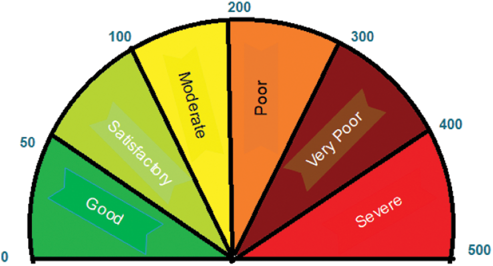
Figure 1: AQI categories as defined by EPA
A report [3] forecasted that 3.3 million annual premature deaths across the world are linked to outdoor air pollution, and this number may double by 2050. The main cause of such events is PM2.5. In India, nearly one million people died in 2015 because of poor air quality [4]. According to the World Air Quality Index project [5], India is among the top 10 countries in the world with poor air quality. In the past few years, Indian cities have featured regularly in the top 20 heavily polluted cities of the world [6,7]. An evidence-based report [8] stated that exposure to fine particulates has serious effects on patients with cardiopulmonary symptoms.
In the context of the increasingly serious health issues caused by the COVID-19 pandemic, researchers have conducted a substantial number of studies forecasting the various air pollutant levels in the ambient air. According to one report [9], when human activities were restricted because of the COVID-19 pandemic in India, PM2.5 levels decreased substantially in most cities. Correlated AQI data in Indian cities, especially in the northern and eastern regions, were better than they had been in years. Following WHO’s air quality guidelines (WHO, 2005), the tolerable values of pollutants such as PM2.5, PM10, O3, NO2, and SO2 are as follows: 25  g/m3 (24-h mean), 50
  g/m3 (24-h mean), 100
  g/m3 (8-h mean), 200
  g/m3 (1-h mean), and 20
  g/m3 (24-h mean). The suggested air quality guidelines for CO are 4 mg/m3 (1-h mean).
Hypotheses to detect the link between COVID-19 lockdown activities and air pollutants are included The 73 meteorological parameters are collected from more than 10,000 air quality stations. The extraordinary restrictions in economic activity caused by the pandemic substantially reduced NOx and PM levels to 60% and 31% in 34 countries, which in turn reduced instances of premature mortality [10]. This shows the importance of proposing alternative solutions for fossil fuel based transport and industry.
Parallel [11] to its rising economic and technological development, China has faced severe air pollution in the past few decades. The report claimed that the COVID-19 lockdown did not reduce air pollution in China. Although there were major emission reduction in transportation and a slight reduction in industry, the meteorology sector was unfavorable during the pandemic period across most parts of the country. This proves that meteorological variation contributes to more air pollution than other activities of a country. Considering the facts presented in the aforementioned sections, a system is needed that can forecast the various pollutants in the air on a monthly or hourly basis. The system should continuously generate data about air pollutants, to infer insight about the same which requires expertise approaches.
Currently, there are two state-of-the-art methods for predicting air quality: (i) statistical models and (ii) artificial intelligence techniques. Statistical models based on single variable linear regression [12] have shown a negative correlation between different variables that influence prediction. Meanwhile, artificial-intelligence-based approaches can include several parameters to facilitate better forecasting. References [13–15] presented artificial-neural-network-based classifiers to forecast pollution from meteorological data. Further, a trend study [16,17] revealed that AI techniques are more reliable in solving forecasting problems. Therefore, most air quality prediction models [18–20] are designed on AI platforms. The efficacy of the model lies in its precise prediction of various levels of air pollutants. The COVID-19 crisis has had a confounding effect on air pollutants.
Outdoor air pollution is mostly due to anthropogenic fine PM (PM2.5). The authors in [21] analyzed PM2.5 using machine learning techniques. Their proposed classification model confirmed the reliability of the classification of three different concentrations of PM2.5. The study made better predictions of PM2.5 using meteorological data of heavy precipitation or strong winds.
Reference [19] developed a system to examine pollutant (CO, SO2, NO, O3, and PM 2.5) concentrations on an hourly basis and predict AQI. The system was based on support vector regression, with radial basis function used as a kernel to make more reliable predictions. The system classified the samples accurately into six categories as per the guidelines of the EPA. In contrast with standard regression models, [22] presented a solution to predict pollutant levels on an hourly basis using multi-task learning (MTL). The MTL model allows one to choose different regularization techniques. Some proposed a few regularization methods, such as the Fresenius norm and nuclear norm that can be used with the model to make more reliable predictions. Reference [23] predicted that the level of PM2.5 can increase by 33% because of restricted activities. Forecasting was simulated using weather research forecasting (WRF) and air quality model (AERMOD). WRF-AERMOD ignored the influence of meteorological variables and unfavorable events in November 2019. The research concluded that the risks associated with PM2.5 declined by 52% in India. Researchers interested in WRF-AERMOD can refer to [24]. A simple, robust model is needed to address current air quality prediction requirements using a fewer number of samples. The model in this paper considers the average AQI values recorded in India to forecast future AQI values. The classification model is trained using AQI values and validated using the results obtained by the forecasting model.
The rest of the paper is organized as follows. Section 2 elaborates on the data preprocessing and data visualization phase for designing a precise model. Section 3 discusses the steps taken to design AQI forecasting models. Section 4 presents an AQI category classification model using machine learning techniques. Section 5 presents future research directions.
2 Data Preparedness and Visualization
A thorough data visualization phase is established to provide insights into data recorded in urban areas in India. This will allow the forecasting and classification model to find prevalent factors.
The dataset is taken from the World Air Quality Index historical data platform [25]. The filtered dataset consists of 29,531 instances for 23 Indian cities. Each data point consists of 16 parameters. Furthermore, the dataset includes several air pollutant concentrations from various cities in India arranged according to date. The recorded samples were collected from January 2015 to July 2020.
In the preprocessing step, unwanted data and null values are removed. The data analysis reveals that there are many missing values. In particular, a few of the city columns have many missing values. In the AQI column, complete data can be found only for Delhi. This is unfortunate because it shows that official records of pollutant levels are not complete. The dataset has a few columns with many missing values removed. These missing data do not influence prediction because the average value of a particular column is used for estimating Indian AQI values among 29,531 instances.
The AQI calculation considers seven pollutant data measures: PM2.5, PM10, SO2, NOx, NH3, CO, and O3. The average values in the last 24 hours are used, with the condition of obtaining at least 16 values. For CO and O3, the maximum values in the last 8 hours are used. Each measure is converted into a Sub-Index based on predefined groups.
2.4 Air Pollutants Pattern Visualization
Air pollutant concentration in India is analyzed using Python 3.6 data visualization tools to gain insights into patterns. The most challenging part of defining the value of AQI is the non-availability of some pollutants. Fig. 2 provides better insights into pollutant levels (CO, O3, and PM2.5) in terms of months and years. The monthly data depicted in Fig. 2 shows the apparent fall in air pollution in July and August. Such an effect may be primarily due to the monsoon season, which occurs during these months. A major decline in air pollution is observed around the month of June, there is then a slow rise to the highest levels during the winter season. This decline, rise, and peak can be attributed to the practice of burning crops in the northern parts of India.
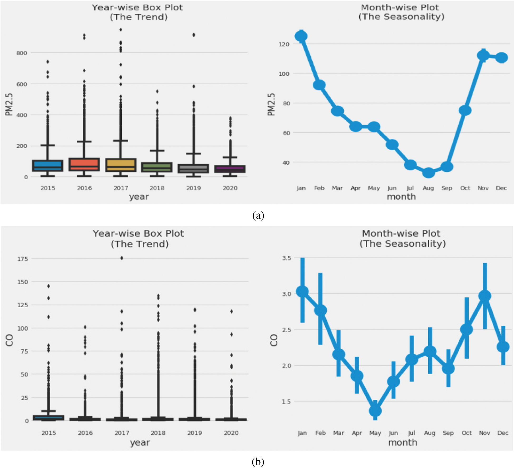
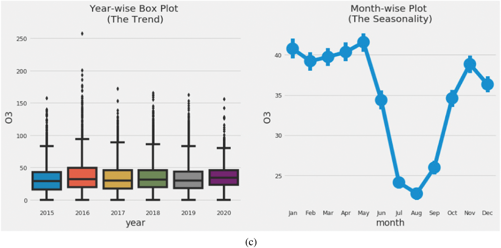
Figure 2: Concentration level measured in terms of months in India. (a) PM2.5 (b) CO (c) O3
Fig. 3a provides a snapshot of the trends observed in AQI values computed for various cities in India. Two highly noticeable patterns can be seen over the years. One is a general downward trend. The other is a marginal reduction in AQI values. Fig. 3b depicts the PM2.5 (pollutant) levels recorded from 2015 to 2020. One can right away see clear patterns and trends over the years. There are two highly noticeable major trends. One is a general downward trend, and the other is an upward trend of a recorded PM2.5 values. Over the past five years, observations regarding the level of PM2.5 reduced marginally. In both cases, the levels of AQI and PM2.5 substantially declined according to the data. This could be a misleading fact given the observations made in Delhi and Ahmedabad in 2015. Therefore, the initial portion of the graphs in Figs. 3a and 3b are highly exaggerated. However, a general decline is observed in PM2.5 pollutant concentration over the years. Figs. 4a and 4b interpret the seasonal decomposition of AQI as well as PM2.5 values observed over the years. The data reveals a clear seasonality, and fewer clear trends can be observed as well. This may be due to the increasing restrictions on pollution imposed by the government. The final major downward surge was undoubtedly due to the recent COVID-19 pandemic. Furthermore, regarding seasonality, the question arises as to what causes an increase during certain months and a decline in others? Regarding the AQI levels depicted in Figs. 4a and 4b, there are two large peaks: the first peak is in October, and the second is in January. The amount of pollution recorded from around July to September is the lowest, after which there is a subsequent sharp increase. Similarly, there is a decrease from January to July due to a combination of winter aversion (explained later); the valley effect (explained later); seasonal factors such as dust storms, crop fires, burning of solid fuels for heating, firecracker-related pollution during the Diwali festival, stubble burning; and so on. North Indian states witness a greater increase in pollution.
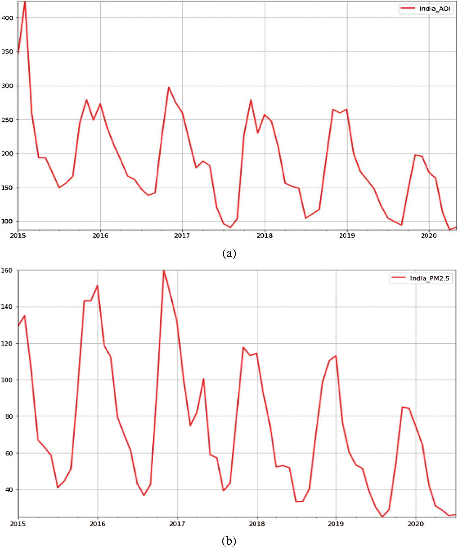
Figure 3: (a) Recorded AQI values from 2015–2020 in India. (b) The recorded concentration of PM2.5 levels from 2015–2020 in India
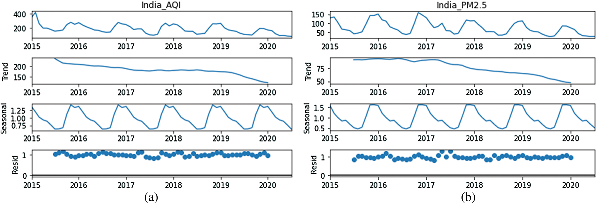
Figure 4: (a) Seasonal decompose of AQI values. (b) Seasonal decompose of PM2.5 in India
During the summer, the air in the lowest part of the atmosphere is warmer and lighter, so it rises in an upward direction. Naturally, the air carries pollutants away from the ground and mixes them with cleaner air in the upper layers of the atmosphere using a process called “vertical mixing.” In contrast, in the winter and monsoon seasons, the air in the planetary boundary layer becomes thinner and the cooler air near the earth’s surface becomes denser. Consequently, the cooler air may get trapped under the warm air above, which forms a kind of atmospheric “lid.” This is referred to as “winter inversion”. The vertical mixing of air occurs only within this layer; the pollutants thus released need enough space to diffuse in the atmosphere. As pollution levels reduce in summer, allowing the warmer air to rise freely, the boundary layer becomes thicker, allowing pollutants to disperse. Similarly, in the winter afternoons; the heat brings down the pollution slightly. The effects of inversion are sharper at night; this is why air quality levels instantly drop overnight. This may also be the reason behind experts requesting people to refrain from early morning walks when they could be exposed to much higher pollution levels. In the coastline areas, sea breeze and moisture disperses pollution. In the Indo-Gangetic Plain, Punjab, Delhi, Uttar Pradesh, Bihar, and West Bengal, the valley is surrounded by the Himalayas and other mountain ranges. Polluted air is therefore locked in the valley and cannot drift around because of low-speed winds. In Delhi and Kanpur, industrial and vehicular emissions coupled with biomass burning increases pollution.
A forecasting model to predict AQI and PM 2.5 values for India is proposed using Seasonal Autoregressive Integrated Moving Average (SARIMA) and Facebook’s Prophet Library. The model is optimized to predict AQI and PM2.5 values for the coming year. Fig. 5 shows the proposed framework of the model.
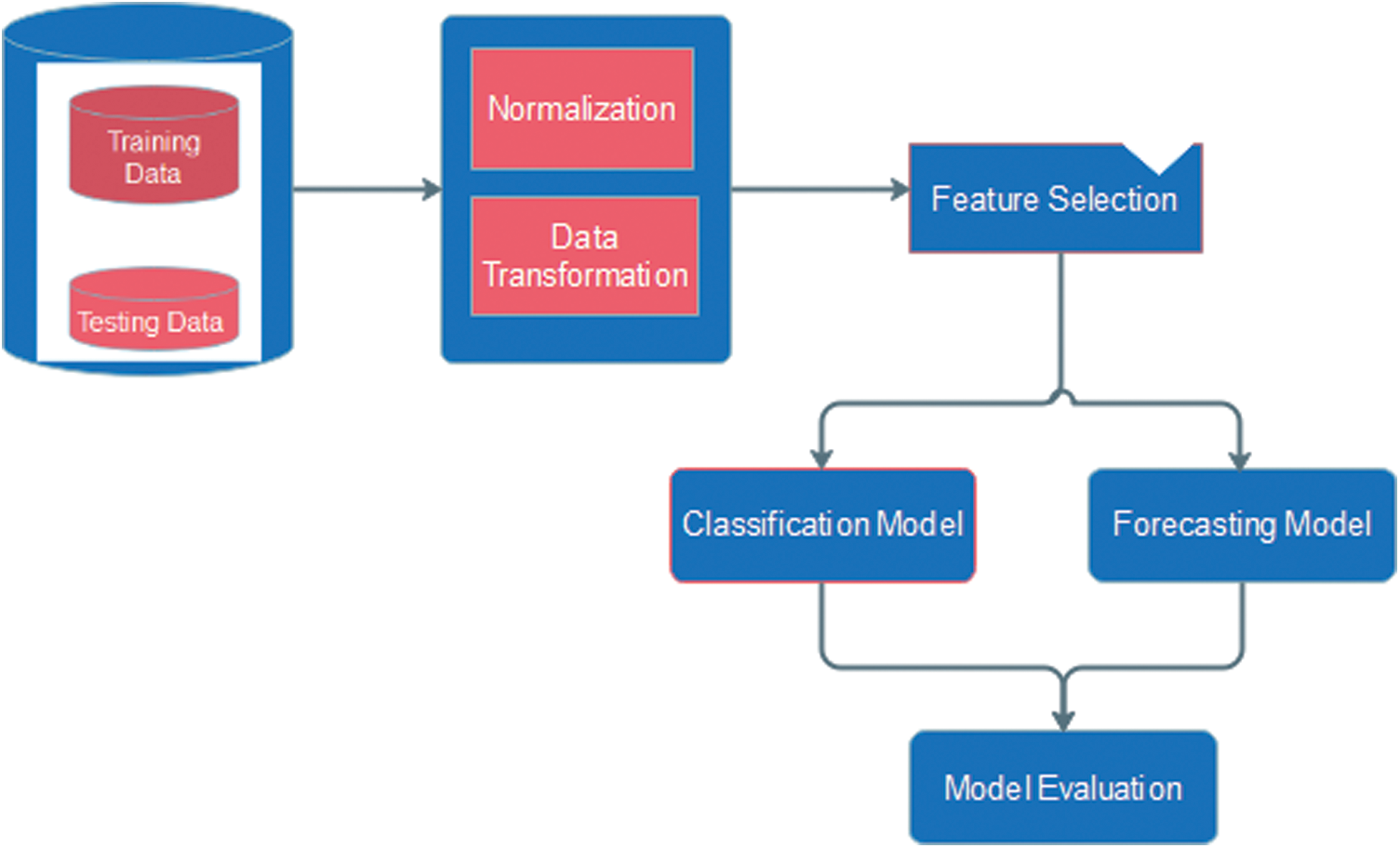
Figure 5: Outline of the proposed framework
To forecast univariate time series data, ARIMA is most preferred. The reason behind this is its inherent ability to handle trends in time series data, so it is applied in various domains. However, ARIMA cannot support time-series data with a seasonal component. An extension to ARIMA (parameters mentioned in Eq. (1)) that supports the direct modeling of the seasonal component of a series is called SARIMA. This is an extension of ARIMA represented in Eq. (2).

where (p,d,q) are non-seasonal part of the model, (P, D, Q) is a seasonal part of the model

where  is Gaussian white noise,
  (B) represents the ordinary autoregressive,
  (B) depicts moving average components,
  (Bs) and
  (Bs) are seasonal autoregressive and moving average components. (
 )d and
  denotes ordinary and seasonal different components of order d and D.
Facebook offers a tool for time series forecasting for some contexts. The Prophet is built using STAN, a probabilistic coding language. Prophet offers the same advantages offered by Bayesian statistics, including seasonality. Prophet uses Python and R to develop its forecasting prototype, thus eliminating the need to develop a wide range of scalable models. The built-in API uses cutting-edge forecasting methods to obtain good-quality forecasting data. The Prophet library enables one to develop a varying degree of models wherein some contexts are quite simple, while others may be too complex. However, Prophet models are fairly non-customizable in terms of the actual modeling as well as visualization; hence, in some cases, the resultant model or data is a less transparent version than SARIMA.
The forecasting models presented in this paper are implemented using Python3.6. The optimal parameters for the customized SARIMAX model are 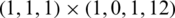 . Here, the numeric value 12 is used to indicate the usage of monthly data. The model does not include an external variable, so it is SARIMA. The model selection criterion is the Akaike’s Information Criterion (AIC) by default. To forecast AQI values, the dataset is divided into training and testing data. The proposed SARIMA model considers AQI values from 2015 to 2018 (till June) as the training dataset, and July 2018 to June 2019 as the test dataset. The reason for excluding 2020 is that the year is an outlier because of COVID-19; therefore, including data from 2020 may deviate from the actual prediction. To demonstrate the efficacy of the designed classifier using the SARIMA model, a snapshot is shown in Fig. 6. The figure shows a comparison between the SARIMA values and the actual values in the month-wise corpus for 2019.
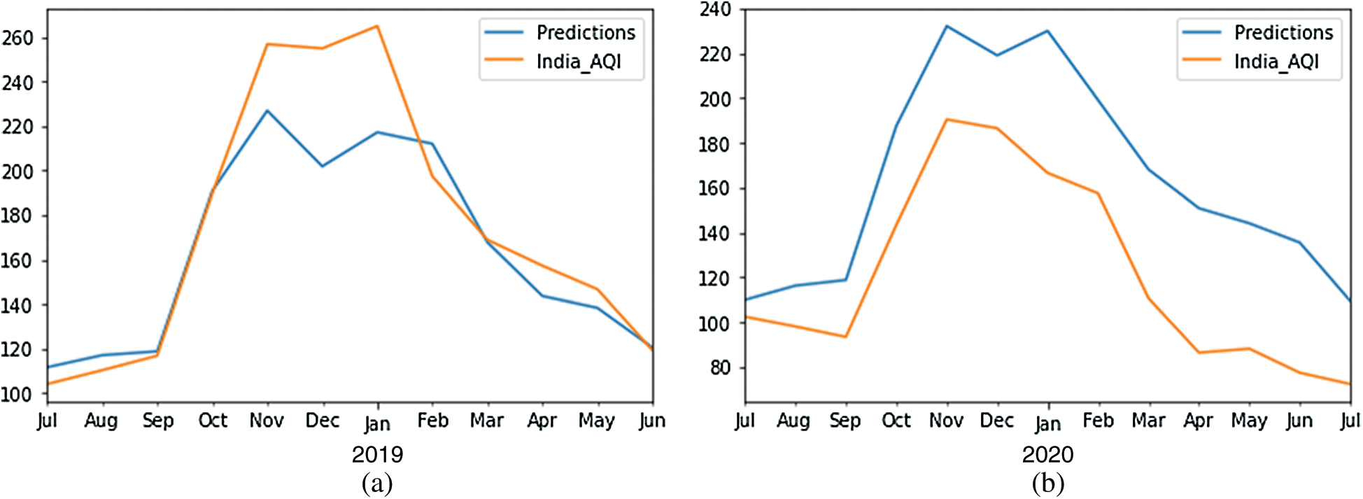
Figure 6: Performance of SARIMA in predicting the AQI values (a) AQI-2019 (b) AQI- 2020
According to Fig. 6a, the predicted values are fairly close to the actual values using SARIMA. It is quite fascinating how looking at previous values gives us so much insight into future air pollution trends. However, there is a discrepancy at the peak of the graph, where our model is unable to make predictions with high accuracy. The SARIMA model predicts AQI values for 2019–2020 (May–July). Fig. 6b shows the month-wise predicted results of AQI through SARIMA for 2020. The resultant data reveals a gap between the actual versus predicted AQI values. Tab. 1 summarizes the SARIMA model’s performance in terms of root mean square error (RMSE), as shown below.

Table 1: Error metrics from AQI forecasting models
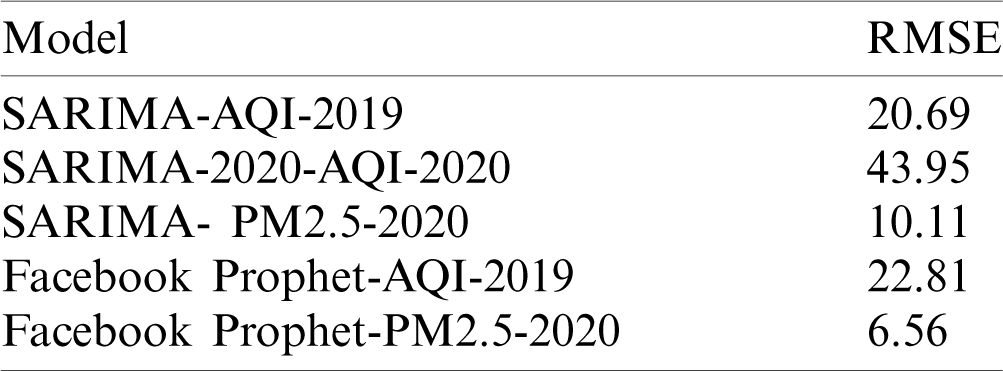
For 2019, an RMSE value of approximately 21 is achieved. While approximately judging the scale of error, the mean value of AQI is 177, so the error is approximately 1/9 of the actual values. Regarding the predicted results for 2020, the error value is much higher than earlier for obvious reasons, which indicates that predicting AQI values for 2020 is not going to yield accurate results.
Prediction for 2020 through SARIMA produces 43.95 as an RMSE value and 133.55 is the average AQI value for 2020. Fig. 7 shows the performance of SARIMA in predicting the PM2.5 values for 2020 and 2021, respectively. The predicted values are fairly close to our actual values obtained using SARIMA. The error value between the existing versus forecasted results is summarized in Tab. 2. In terms of RMSE, the value is 10.11, and the average PM2.5 value is 5.51. In the next phase, the forecasting of PM2.5 values through SARIMA is carried out and plotted in Figs. 8a and 8b respectively. Predicting the levels of AQI and PM2.5 using SARIMA for the upcoming year (2020–2021) is however difficult for analysts and researchers. If a predictive model considers 2020 data, there may be a chance of inaccurate prediction by the model for next year because 2020 is an outlier.
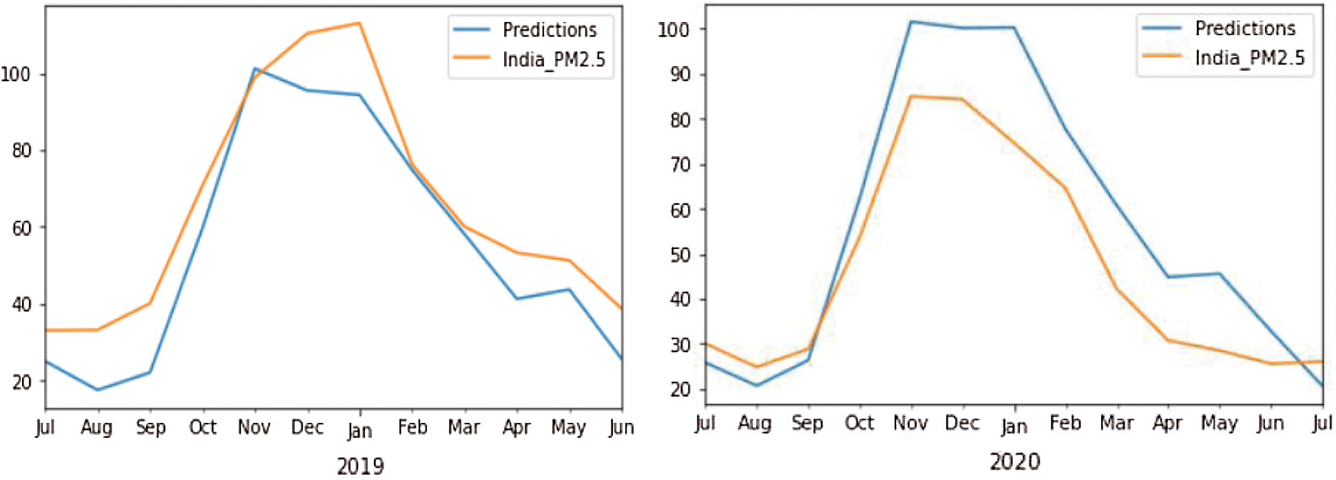
Figure 7: Predicted PM2.5 values from SARIMA for the period Mid 2019–Mid 2021
Table 2: AQI classifier Performance in terms of TPR and FNR
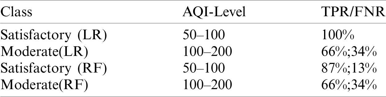
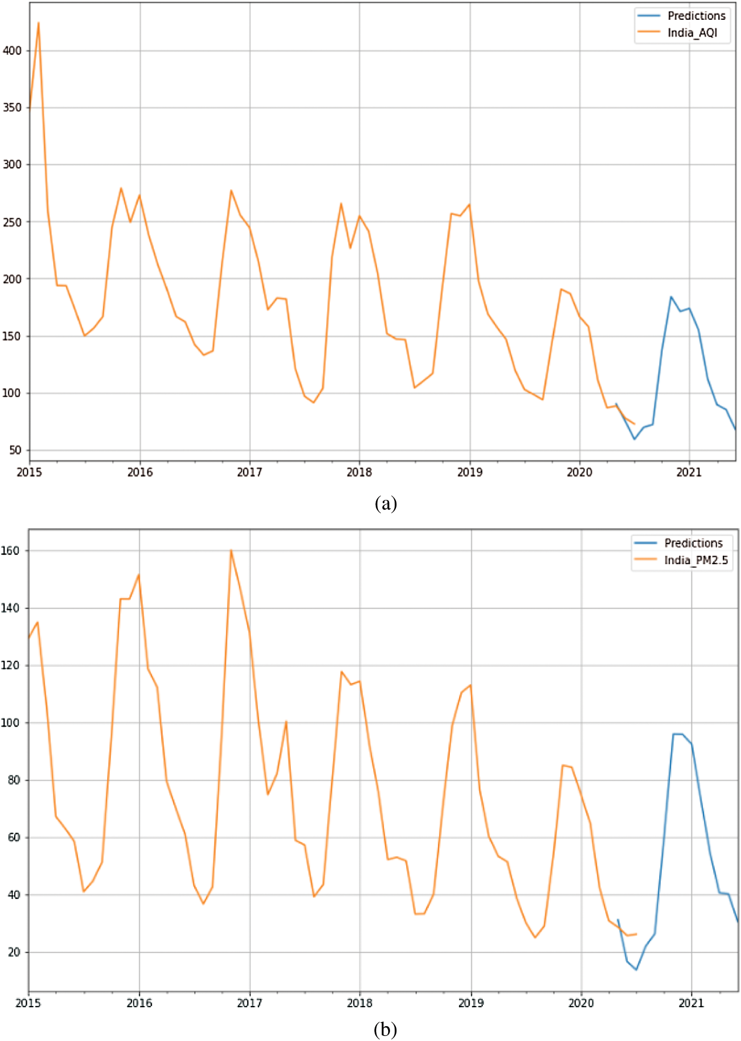
Figure 8: (a) Forecasted AQI values through SARIMA for the year 2020–2021 (b) Forecasted of PM2.5 values through SARIMA for the year 2020–2021
However, not including the 2020 data in our dataset might lead to wrong predictions, and COVID-19 could have lasting effects that could lead to poor predictions. Consequently, the presented forecasting system for AQI values includes 2020 data, and the forecasted results are highly optimistic. Further, this scenario is pure since 2020 is an outlier. If pollution levels follow the trend before 2020, this would mean a bump in AQI levels unless the country restricted anthropogenic activities to a great extent. A better prediction may be possible by skipping 2020. Fig. 8a shows the AQI values forecasted using SARIMA for 2020–2021. Fig. 8b shows the PM2.5 values for 2020–2021.
Regarding the data forecasted using Facebook’s Prophet, Figs. 9a and 9b depict the predicted results of AQI and PM2.5 for 2019. In terms of quantitative metric RMSE, the SARIMA model results are better than the Facebook Prophet results in making predictions for 2019.
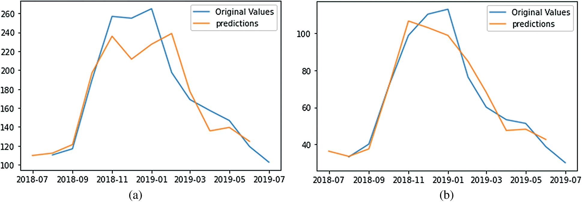
Figure 9: The actual versus predicted the values of (a) AQI and (b) PM2.5 values through Facebook Prophet
For PM2.5 prediction, Facebook’s Prophet performs better than SARIMA; this can be verified in Tab. 2. Prophet fares better than SARIMA because of its inherent ability to handle data trends that have not been too greatly altered by COVID-19. This seems to indicate that Prophet places more emphasis on past values compared to SARIMA.
The forecasted values against the AQI and PM2.5 can be found in Figs. 10a and 10b. The black dot (change points) shows positions where sudden and abrupt changes occur in the trend. Consider the following analogy; an online campaign suddenly receives 50,000 more constant visitors to its website. Here, the change point will be the timeslot where this major change occurred. Prophet renders data using 25 potential change points, where all of them were uniformly placed in the first 80% of the time series. The blue shaded area in Figs. 10a and 10b shows approximate predicted values in the upper range and lower range. The correctness of the prediction can be verified by comparing the forecasted results for 2018 and the RMSE values in Tab. 1. While forecasting AQI values for 2019, SARIMA outperformed Prophet. However, while forecasting PM2.5 values for 2020, Prophet outperformed SARIMA, as can be verified in Fig. 11.
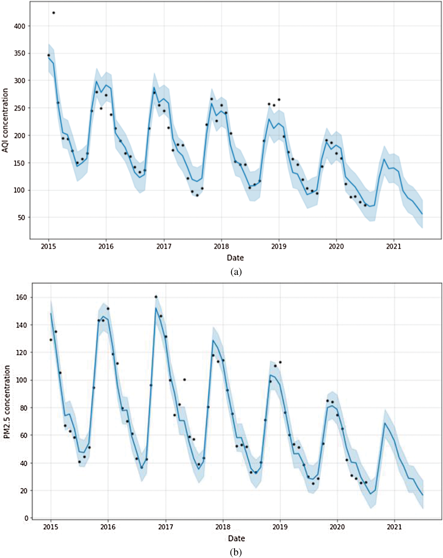
Figure 10: (a) AQI values forecasted according to year through a prophet for 2020–2021 (b) PM2.5 values forecasted according to year through a prophet for 2020–2021
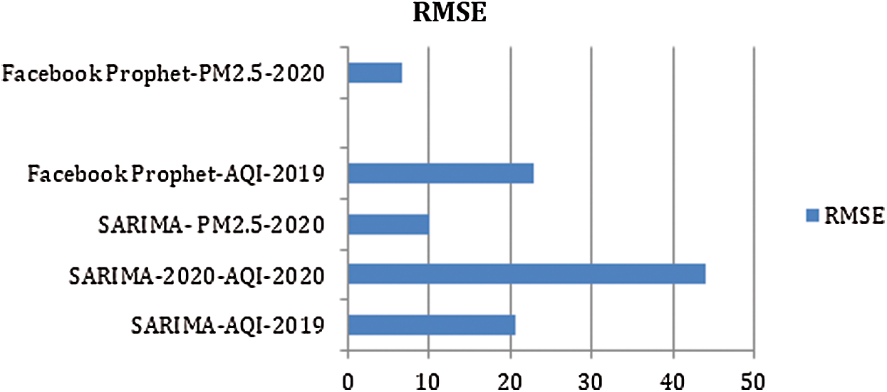
Figure 11: Error metrics obtained through SARIMA and Prophet for 2019 and 2020
The AQI level classification model with various machine learning techniques is discussed in this section. AQI values can be computed as mentioned in the feature selection phase. Cities’ air quality level grading is done qualitatively as per the threshold values suggested by the EPA (Fig. 1). Since the size of datasets is small, machine learning is the perfect choice to implement classification models. The average monthly data computed against AQI values are fed into the classification models. After the encoding process, 80% of the data are used for training and 20% of the data are used for testing. To validate the model, data forecasted by the proposed model is used to verify the robustness of the model. The upcoming section discusses the AQI classification model using logistic regression (LR) and random forest (RF).
LR is a perfect tool where the output class boundary is based on the threshold. The result of the classifier is purely reliant on a threshold value. The output class (Yi) is determined based on  0 and
0 and  1 population intercept and slope. The input feature is represented as Xi. The output classification process through LR is mentioned in Eq. (4)

The proposed AQI classification model is a multiclass classification, so the logistic classifier  (x) for the output class i is used to predict the probability
  . For unseen input x, the proposed classifier chooses class i that maximizes the value of Eq. (5).

RF is an ensemble learning method for classification and regression a task because of its simplicity and diversity, the RF has thus become the most widely used method for simulating a real-time system. The bagging technique is used for reducing the variance of an estimated prediction function. The objective of bagging is to average many noisy but approximately unbiased models. Trees are the resultant ideal candidates for bagging. For each decision tree, entropy is computed using Eq. (6) to achieve information gain.

Let us assume  be the class prediction of pth random forest tree. Then,

4.3 Results and Performance Discussion
The AQI level classification models are designed using a machine learning library in Python 3.6 and trained with average monthly AQI values recorded in an urban area in India. The model cannot find many samples to train the required number of categories. The real problem is a six-class classification and validated using the results forecasted by SARIMA. The forecasted resultant samples shuttle between two categories: Satisfactory and Moderate. To measure the efficacy of the proposed AQI classifier, the metrics True Positive Rate (TPR), False Negative Ratio (FNR), Precision, Recall, F1-Score, and Accuracy are established.
The AQI-category classification model predicts results using LR and RF, as displayed in Tabs. 2 and 3. In Tab. 2, the efficacy of the AQI classifier is portrayed in terms of TPR and FNR. As the forecasted sample represents the two categories of Satisfactory and Moderate, the metric also reveals the data by considering each category on its own. In this two-class classification, for the satisfactory category, the LR obtains 100%, and for the moderate category, it obtains 66% as the TPR value. Therefore, the FNR value is 34%. The output of LR is better than the output of RF. For a satisfactory class, the predicted TPR is 87%, and FNR is 13%. Moderate class prediction is fulfilled with 66% for TPR, and 34% for FNR. The same is represented graphically in Fig. 12a. In Tab. 3, the overall performance of the classifier is measured using Precision, Recall, F1-Score, and Testing Accuracy. The LR method outperforms RF in terms of Recall, F1-Score, and Accuracy. The results of both classifiers are comparable in terms of precision, as Fig. 12b shows.
Table 3: AQI classifier performance in terms of Precision, Recall, F1-Score, and Accuracy
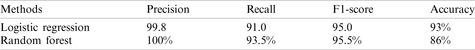
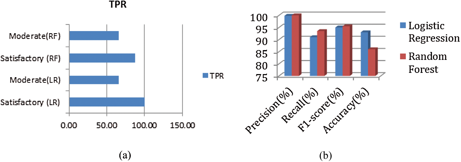
Figure 12: (a) Two class classification using LR and RF (b) performance metrics
Many statistical tools and semi-automated tools help researchers predict air quality by considering several pollutants and seasonal parameters. However, an automated machine learning model to forecast and monitor air quality is required, especially in urban areas. COVID-19 restricted human activities in 2020, and the air quality level significantly improved. Existing models failed to account for this improvement while forecasting the value of AQI. This paper presents a model to forecast AQI and PM2.5 values in India for the coming year by considering surge reduction in various pollutant levels. The proposed model can help regulatory bodies to make predictions. Additionally, a two-class classification model is demonstrated using LR and RF for classifying AQI levels into possible categories as per the threshold level suggested by EPA. However, because of the lack of samples in the dataset, the proposed AQI classifier is downsized to a two-class classifier from a six-class classifier. Experts claim that maintaining PM2.5 under the level specified by the EPA is mandatory to reduce acute respiratory syndrome cases. Results show that the model’s performance is impressive, with 93% accuracy in AQI level classification. The performance of the forecasting model is no worse than that of the classification model. In terms of error metrics, the forecasting model produces minimal values; this may guarantee precise predictions. The proposed models are designed using machine learning methods with optimal hyperparameters. In the future, the same work can be simulated through deep learning architecture.
Acknowledgement: The authors extend their heartfelt gratitude to King Abdul-Aziz City for Science and Technology (KACST) and Umm Al-Qura University for funding this work through the researchers’ supporting project number (14-INF1015-10).
Funding Statement: The work was funded by grant number 14-INF1015-10 from the National Science, Technology, and Innovation Plan (MAARIFAH), the King Abdul-Aziz City for Science and Technology (KACST), Kingdom of Saudi Arabia. We thank the Science and Technology Unit at Umm Al-Qura University for their continued logistics support.
Conflict of Interests: The authors declare that there is no conflict of interests.
1. United Nations, Department of Economic and Social Affairs, 2018. Available: https://www.un.org/development/desa/en/news/population/2018-revision-of-world-urbanization-prospects.html, Accessed Date: 7 September 2020. [Google Scholar]
2. M. A. Pohjola, A. Kousa and J. Kukkonen. (2002). “The spatial and temporal variation of measured urban PM10 and PM2.5 in the Helsinki metropolitan area,” Water Air and Soil Pollution: Focus, vol. 2, no. 5, pp. 189–201. [Google Scholar]
3. J. Lelieveld, J. S. Evans, M. Fnais, D. Giannadaki and A. Pozzer. (2015). “The contribution of outdoor air pollution sources to premature mortality on a global scale,” Nature, vol. 525, no. 7569, pp. 367–371. [Google Scholar]
4. H. Guo, S. H. Kota, S. K. Sahu, J. Hu and Q. Ying. (2017). “Source apportionment of PM2. 5 in North India using source-oriented air quality models,” Environmental Pollution, vol. 231, pp. 426–436. [Google Scholar]
5. World Air Quality: Air Quality Rankings, Available: https://www.iqair.com/us/world-most-polluted-countries, Accessed Date: 7 September 2020. [Google Scholar]
6. R. Garaga, S. K. Sahu and S. H. Kota. (2018). “A review of air quality modeling studies in India: Local and regional scale,” Current Pollution Reports, vol. 4, no. 2, pp. 59–73. [Google Scholar]
7. A. Mukherjee and M. Agrawal. (2018). “Air pollutant levels are 12 times higher than guidelines in Varanasi,” India Sources and transfer, Environmental Chemistry Letters, vol. 16, no. 3, pp. 1009–1016. [Google Scholar]
8. C. A. Pope and D. W. Dockery. (2006). “Health effects of fine particulate air pollution: Lines that connect,” Journal of the Air and Waste Management Association, vol. 56, no. 6, pp. 709–742. [Google Scholar]
9. S. Sharma, M. Zhang, J. Gao, H. Zhang and S. H. Kota. (2020). “Effect of restricted emissions during COVID-19 on air quality in India,” Science of the Total Environment, vol. 728, pp. 138878. [Google Scholar]
10. Z. S. Venter, K. Aunan, S. Chowdhury and J. Lelieveld. (2020). “COVID-19 lockdowns cause global air pollution declines with implications for public health risk,” medRxiv. [Google Scholar]
11. P. Wang, K. Chen, S. Zhu, P. Wang and H. Zhang. (2020). “Severe air pollution events not avoided by reduced anthropogenic activities during COVID-19 outbreak,” Resources, Conservation and Recycling, vol. 158, pp. 104814. [Google Scholar]
12. Y. Li, Q. Chen, H. Zhao, L. Wang and R. Tao. (2015). “Variations in pm10, pm2.5 and pm1.0 in an urban area of the sichuan basin and their relation to meteorological factors,” Atmosphere, vol. 6, no. 1, pp. 150–163. [Google Scholar]
13. X. Ni, H. Huang and W. Du. (2017). “Relevance analysis and short-term prediction of PM2.5 concentrations in Beijing based on multi-source data,” Atmospheric Environment, vol. 150, pp. 146–161. [Google Scholar]
14. J. Chen, H. Chen, Z. Wu, D. Hu and J. Z. Pan. (2017). “Forecasting smog-related health hazard based on social media and physical sensor,” Information Systems, vol. 64, pp. 281–291. [Google Scholar]
15. J. Zhang and W. Ding. (2017). “Prediction of air pollutants concentration based on an extreme learning machine: The case of Hong Kong,” International Journal of Environmental Research and Public Health, vol. 14, no. 2, pp. 114. [Google Scholar]
16. F. Zhang, H. Cheng and Z. Wang. (2014). “Fine particles (PM2.5) at a CAWNET background site in central China: Chemical compositions, seasonal variations and regional pollution events,” Atmospheric Environment, vol. 86, pp. 193–202. [Google Scholar]
17. X. Xi, Z. Wei and R. Xiaoguang. (2015). “A comprehensive evaluation of air pollution prediction improvement by a machine learning method,” in In. Proc. IEEE, Tunisia, pp. 176–181. [Google Scholar]
18. C. Brokamp, R. Jandarov, M. B. Rao, G. LeMasters and P. Ryan. (2017). “Exposure assessment models for elemental components of particulate matter in an urban environment: A comparison of regression and random forest approaches,” Atmospheric Environment, vol. 151, pp. 1–11. [Google Scholar]
19. M. Castelli, F. Clemente, A. Popvic, S. Silva and L. Vanneschi. (2020). “A machine learning approach to predict air quality in California,” Complexity, vol. 2020,Article ID 8049504,23 pages. [Google Scholar]
20. M. A. Cole, R. J. Elliott and B. Liu. (2020). “The impact of the Wuhan Covid-19 lockdown on air pollution and health: A machine learning and augmented synthetic control approach,” Environmental and Resource Economics, vol. 76, no. 4, pp. 553–580. [Google Scholar]
21. J. Kleine Deters, R. Zalakeviciute, M. Gonzalez and Y. Rybarczyk. (2017). “Modeling PM2. 5 urban pollution using machine learning and selected meteorological parameters,” Journal of Electrical and Computer Engineering, vol. 2017, Article ID 5106045,14 pages. [Google Scholar]
22. D. Zhu, C. Cai, T. Yang and X. Zhou. (2018). “A machine learning approach for air quality prediction: Model regularization and optimization,” Big Data and Cognitive Computing, vol. 2, no. 1, pp. 5. [Google Scholar]
23. A. S. Sharma, M. Zhang, J. Gao, H. Zhang and S. H. Kota. (2020). “Effect of restricted emissions during COVID-19 on air quality in India,” Science of the Total Environment, vol. 728, pp. 138878. [Google Scholar]
24. R. S. Kumar, A. K. PatilDikshit and R. Kumar. (2017). “Application of WRF model for air quality modeling and AERMOD-a survey,” Aerosol and Air Quality Research, vol. 17, no. 7, pp. 1925–1937. [Google Scholar]
25. Air Quality Open Data Platform Worldwide COVID-19 dataset, Available: https://aqicn.org/data-platform/covid19/report, Accessed Date: 2 September 2020. [Google Scholar]
 | This work is licensed under a Creative Commons Attribution 4.0 International License, which permits unrestricted use, distribution, and reproduction in any medium, provided the original work is properly cited. |