DOI:10.32604/cmc.2021.015159
| Computers, Materials & Continua DOI:10.32604/cmc.2021.015159 | |
| Article |
Transmission and Reflection of Water-Wave on a Floating Ship in Vast Oceans
Department of Mathematics, Faculty of Applied Science, Umm Al-Qura University, Makkah, Saudi Arabia
*Corresponding Author: Amel A. Alaidrous. Email: dr.amllah_gol@hotmail.com
Received: 08 November 2020; Accepted: 15 December 2020
Abstract: In this paper, we study the water-wave flow under a floating body of an incident wave in a fluid. This model simulates the phenomenon of waves abording a floating ship in a vast ocean. The same model, also simulates the phenomenon of fluid-structure interaction of a large ice sheet in waves. According to this method. We divide the region of the problem into three subregions. Solutions, satisfying the equation in the fluid mass and a part of the boundary conditions in each subregion, are given. We obtain such solutions as infinite series including unknown coefficients. We consider a limited number only of the coefficients by truncating the infinite series and satisfy the remaining boundary conditions approximately. Numerical experiments show that the results are acceptable. Tables are given along with the graph of the system of the resulting streamlines and the dynamical pressure acting on the obstacle. The drawn system of streamlines shows the correctness of the solution and the pressure is maximum on the side facing the upstream extremity of the channel. The same procedure can be adequately applied for problems with more complicated geometry and other phenomenon can thus be simulated.
Keywords: Potential flow; linear theory; fixed floating obstacle; fourier transformation; boundary collocation technique; spectral method
The problem of the study of water-wave flow under an upper fixed floating obstacle is very important from theoretical and experimental points of view. This model simulates the phenomenon of waves falling on a floating ship in a vast ocean. The class including this type of problem is called the class of Cauchy–Poisson Problems (CPP).
This class of problems simulates several phenomena having geophysical interests. These models simulate the phenomenon of waves abording a floating ship in a vast ocean. The same models, also simulate the phenomenon of fluid-structure interaction of a large ice sheet in waves. We can find a discussion of this issue in [1–4]. These problems are non-linear, mixed free boundary value problems. Certain specified initial conditions may be assumed to these free boundary value problems [5,6]. Several difficulties envisage the theoretical study of these mathematical models. The non-linearity of the model and the fact that the free surface is not known from the outset are some of these difficulties. Other difficulties are represented in the irregularity of the geometry of the region of the problem.
To overcome the non-linearity difficulty, the problem is treated following theories of long waves or the shallow water [7–10]. The linear theory of motion and theories of higher orders may be adopted [4,11]. Researchers usually use perturbation techniques to concur the difficulties coming from the irregularity of the region of the problem and approximate analytical solutions are sought. One may carry out the perturbation around a vertical or a horizontal line [7–9,12–16] regarding the particular geometry of the studied problem. It is impossible to obtain exact analytical solutions once the geometry deviates from being simple and other additional conditions are to be assumed on the geometry in order to obtain approximate analytical solutions. These additional conditions may include the assumption of thin barriers [7–9], or that of infinite depth [16], or mild slope and short topographies [11,13–15].
Numerical techniques are other alternatives if the analytical approach is inadequate. For a review of the numerical methods applied to CPP see [17,18] and references included. However, numerical procedures have their difficulties. These difficulties are appearing in convergence, stability, consistency, and error accumulation and need huge computations.
The spectral methods are semi-analytical methods used for the solution. Trefftz method [19,20], the procedures of perturbation [11,21], the boundary integral techniques [22,23], and the method of fundamental solutions [24] are examples of the semi-analytical methods. An original method for the study of flow over topography is given in [25]. This method is classified as a semi-analytical one.
The phenomenon of scattering of waves by an immersed or floating barrier in deep or in shallow water is a subject that attracts the attention of several authors (see for example, for analytical study [7–9], [25–34], for numerical study [29,35,36] and for experimental study [28,29,37–41]).
We follow here the method introduced by Abou-Dina et al. [25] for the study of water-wave flow under a fixed floating obstacle and for discovering the behavior of the resulting flow. Following this technique, the region of the definition of the problem is divided into three sub-regions. One of these regions contains a fixed floating body. We express the solutions satisfying the equations and conditions in the semi-infinite sub-domains with a set of unknown coefficients and elementary harmonic functions. The velocity potential function in the subdomain containing the obstacle is extended analytically through the boundary of the floating obstacle. We give a general solution in the enlarged sub-domain by applying the finite cosine Fourier transform. This solution uses another set of arbitrary constants and satisfies the system of equations and conditions on the horizontal bottom. We express the solution in the three subregions using one set only of coefficients by applying the continuity of the remaining physical quantities. This solution satisfies the system of equations and conditions of the problem except those on the fixed floating obstacle and probably on a part of the free surface. We satisfy these latter conditions and hence we get an equation in the form of a series to be fulfilled on the boundary of the obstacle and on the considered part of the free surface if necessary. The coefficients are obtained as a solution of a system of linear equations. Acceptable results obeying a certain specified error measure are given for the particular case of an obstacle with a sinusoidal boundary.
The application, dealing with this boundary of the fixed floating obstacle, ascertains the efficiency of applying this procedure for the solution. The drawn system of streamlines shows the correctness of the solution and the dynamical pressure acting on the witted surface of the fixed floating obstacle is exhibited graphically. The pressure is found to be maximum on the side facing the incident wave and decreases till attaining its minimal values on the other side.
The problem is described by an infinite channel of finite depth. This channel is occupied by a fluid layer of constant density. The fluid layer is bounded from above and from below by a free surface and an impermeable horizontal bottom, respectively. A floating obstacle of arbitrary shape is partially immersed at the free surface (Fig. 1). The fixed floating barrier partially obstructs a wave propagating in the fluid. The incident wave is harmonic with frequency denoted by  . This situation generates transmitted and reflected waves and local perturbations as well. It is required to find the coefficients of the transmission and the reflection. The local oscillations are also to be determined. The problem is studied in two dimensions. The study is carried out following the first-order theory of motion, the fluid is considered ideal and a velocity potential is assumed. We use the Cartesian frame, shown in Fig. 1. The origin of the system of coordinates is chosen in the mean horizontal line of the upper bound of the fluid, the x-axis and the y-axis are taken as shown in the figure.
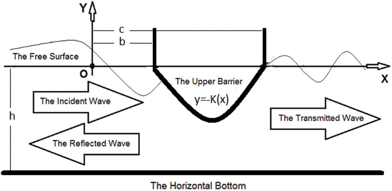
Figure 1: Description of the problem
3 System of Equations and Conditions
The horizontal line y = 0, 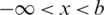 ,
,  and the boundary of the immersed section of the floating obstacle y = − K(x),
  construct higher bound of the region of the study following the linear theory. The time-independent velocity potential
  is defined in terms of the time-dependent one
  as
as

This function satisfies the system [39]:


With the obvious condition that the incident wave is the only wave coming from infinity. The time-dependent functions  and P*(x, y, t), are given respectively as,

and

 and
and  are given as:

and

 is given as

 and
and  satisfy the relations

 is a unit vector parallel to the z-axis.
We follow the method presented by Abou-Dina et al. [6] to get a solution for the above system of equations and conditions.
The region bounded by x = 0 and x = a contains the floating barrier. The region of the problem is thus divided into three subregions: V− , V0, and V+ as shown in (Fig. 2).
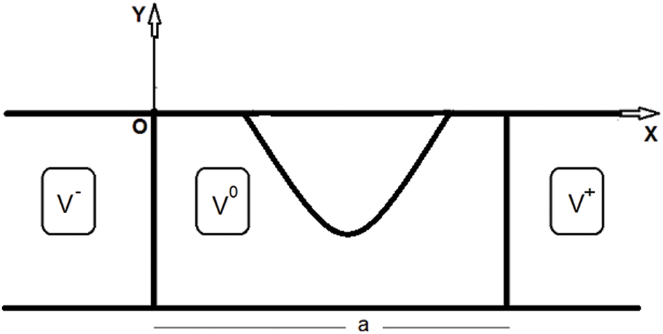
Figure 2: The three subregions V− , V0, and V+
We will solve the problem and the solution includes certain unknown coefficients. The equation in the fluid mass and a part of the boundary conditions are satisfied by this solution. Applying the continuity of the physical quantities at x = 0 and x = a will relate the solutions in the neighboring subregions. We determine the unknown coefficients approximately.
4.1 Study in the Semi-Infinite Domains
Applying the method of separation of variables for the solution of the system of equations and conditions in the regions V− and V+ the solution is obtained in these semi-infinite regions respectively as [5,6]

and

where  denotes the root of the equation

and  denote the roots of the equation

I0, R0, and T0 are the amplitudes of the incident, the reflected and the transmitted waves respectively. Rp and Tp are complex constant coefficients. The obtained solution includes progressive waves going towards the channel extremities and local perturbations decaying in going away from the obstacle. It is required to calculate the coefficients R0, T0, Rp and Tp.
 is the potential in the area V0. This function satisfies Laplace’s equation in V0 and is continuous on
  . The function
  is constant on the boundary of the floating barrier. Therefore, the function
  can be extended on the area OABC of Fig. 3. The extended function is harmonic on the extended region and is denoted by V. If the domain of the problem is multi connected, i.e., it contains holes then this holes are removed and replaced by suitable sources (logarithmic sources) and this has been studied in [27]. Also if there is an external pressure acting on the free surface [22] or a finite part the bottom of the channel is set in motion, the same procedure is applied but the control region V is enlarged to include the parts of the external pressure or the moving bottom.
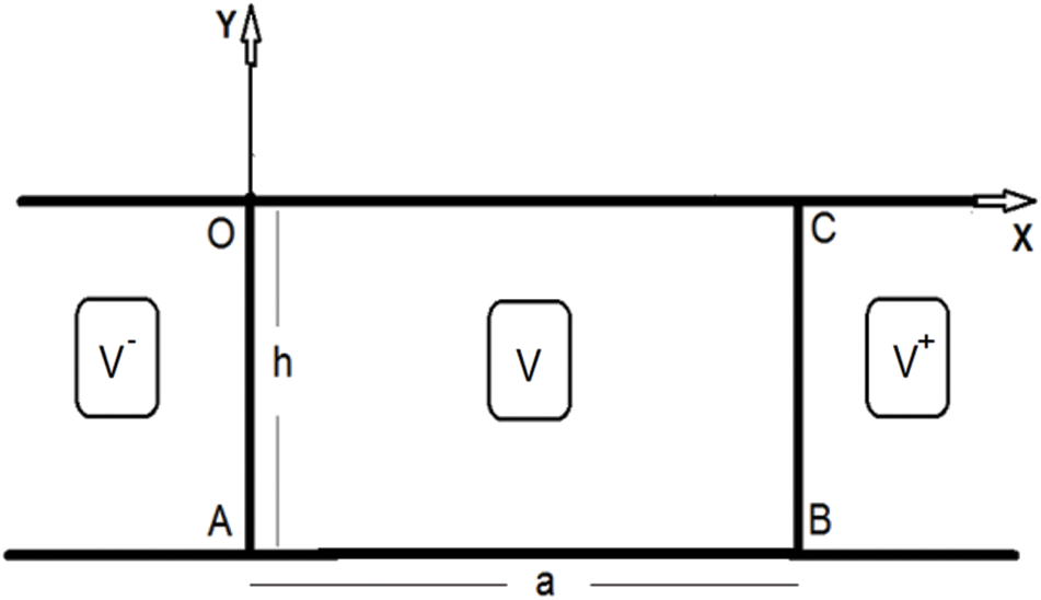
Figure 3: The extended domain
The extended function will also be denoted by  . The system of equations and conditions satisfied by function
  is given as:


and

We use the transform  of
of  defined as [42]:

Applying this transformation to Eqs. (16), (18) and (20)–(22), the functions  ,
,  are obtained after some manipulation in terms of constant coefficients am as
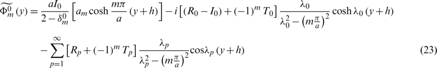
The finite Fourier transform (23) has the following inversion expression [42]:

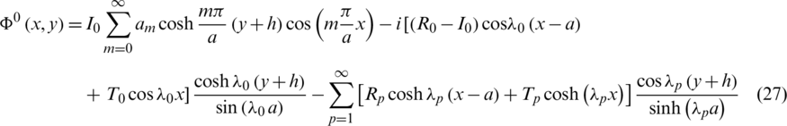
Using (23) and (24) together with the expressions

and

the velocity potential in the domain V0 is obtained as
Substituting expression (27) of  into conditions (17) and (19), we get the following relations
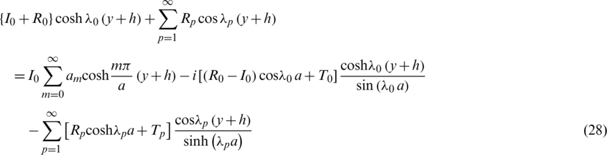
and
The orthogonality of the functions  , over
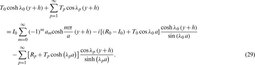
  , is used. The coefficients R0, T0, Rp and Tp,
  are obtained by the use of relations (28) and (29), in the form:


and

where  and
and  are given for
  . and
. and  . as
. as

and

The function  given by (27) is written using (30)–(33) in terms of am,
  as
as

where  ,
,  are given as:
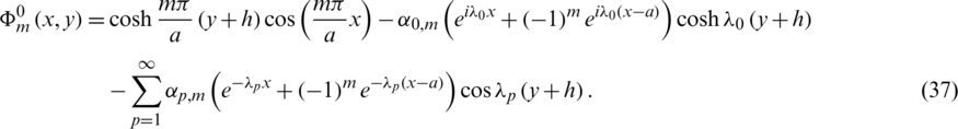
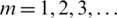
The functions  ,
,  and
and  are obtained from relations (11), (14), (15), (36) and (37) as


and

The functions  ,
,  are defined as
It can be shown using expressions (14) and (15) together with the boundary conditions on the upper and lower bounds of the control region V0 that

Eq. (42) translates the conservation of energy. The conservation of mass is satisfied if

which becomes an identity, if we set

where k > 0 is an integer. k > 0 is taken as the smallest integer (k0) making the sub-domain V0 enclose the fixed floating obstacle.
To get the functions  and
and  , in the whole region of the problem, in terms of am,
  0, we collect relations (14), (15) and (36) for
  and (38)–(40) for
  . These functions satisfy the equations of the problem except the condtion on the higher bound of V0 (see Fig. 2). We satisfy this condition approximately to determine am,
As shown in Fig. 2, the upper bound of the sub-domain V0 consists of two parts of the free surface lying on both sides of the floating obstacle, precisely at  and
and  , in addition to a third part represented by the lower boundary of the obstacle with equation y = − K(x),
  . In the frame of the linear theory of motion adopted here, the condition on the free surface, at
  and
and  , reduces to

which together with expression (36) lead to the following constraints posed on am, 
 are defined by (37). Relations (46) are simplified as

On the other hand, the function  , given by (43)–(45), should have a constant value on the boundary of the floating obstacle
  since this boundary is a part of a certain streamline. Therefore, the coefficients am has also to obey the following series equation

where C0 denotes the constant value taken by the stream-function  on the barrier with equation
 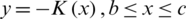 (see Fig. 1 for the constants b, c). Let x0 be a point arbitrarily chosen in the interval
  with y0 = − K(x0). Condition (48) may be replaced by the following
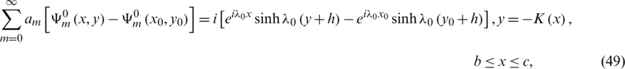
If the floating obstacle occupies the interval  , and no part of the free surface is enclosed in this interval then expression (49) only is to be considered and expressions (47) are discarded. We hence give the solution to the problem in terms of a set of coefficients am. To determine the coefficients of expressions (47, 49), we follow the collocation procedure [39,40]. We replace the infinite upper limit of the series on the L.H.S. of both expressions (47) and (49) by M has taken sufficiently large according to the desired accuracy. We choose a decomposition
  for
for  such that
  , where N is an integer with N > M. We thus obtain the following system of equations

The elements Bm, n and Dn are

and

We have a number N of linear Eqs. (50)–(52) in a number M of the coefficients  with N > M. We put this system in the following square form

where  is the vector of unknown coefficients
  ,
,  is the transpose of the matrix
  and
and  is the vector of constants Dn. The solution of the system (53) determines the velocity potential
  and the stream-function
  , in the sub-region V0 as

and

respectively.
The function  given by (54) satisfies approximately a relation of the form (45) and the function
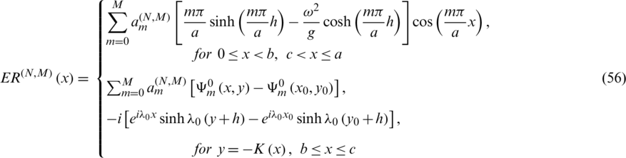
  given by (55) has approximately a constant value along the boundary of the immersed part of the obstacle. We introduce ER(N, M)(x),
  , as local error with:
By checking the inequality

for a control parameter  , the choice of N and M can be controlled. Also, this can be done by checking another inequality of the form

We start with a choice of N and M, then if (4.46) (or (4.47)) is not satisfied, the values of N and M are increased, and we restart the technique to obtaining the desired result. The straight forward collocation technique is met by setting N = M + 1.
Approximate expressions for R0 and T0 are then given as

and

respectively.
5 Numerical Experiments for a Floating Obstacle of a Sinusoidal Boundary
As a numerical experiment, we consider the case of a fixed floating obstacle with a lower immersed part of a sinusoidal boundary with H as a maximum depth and width W. K(x) is considered as

The constant k0 is chosen such that  . k0 is the smallest integer satisfying this relation in such a way that the finite sub-domain V0, lying in the middle with the width a, encloses the fixed floating obstacle (see Fig. 2). Here, we considered the parameters of Fig. 1 as b = 0 and c = W, and Fig. 4 shows the boundary of the floating obstacle in such a case. This curve represents the witted part of the boundary of the floating ship.
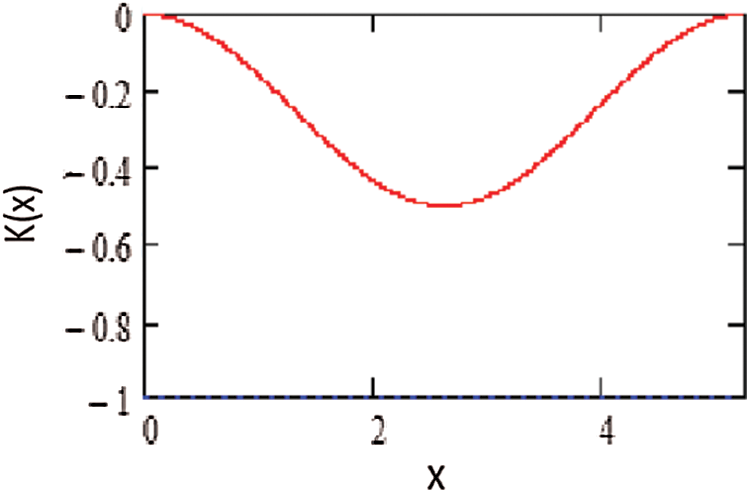
Figure 4: The upper bound of the region V0
We find the error  for some choices of the numbers M and N in Tab. 1. The numerical values given to the different parameters are taken as
  , H/h = 0.5 and W/h = a/h = 5.2373. The value of
  is 1.1997 and we have taken k0 = 1 which results
  as required. The nodes
 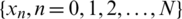 in
in  are assumed equidistant.
Table 1: The errors  for the fixed floating obstacle of Eq. (58)
Tab. 1 indicates that, the efficiency of the method is in general acceptable and that for  , the error oscillates between 10−8 and 10−6. The values N = 250 and M = 290 give the best result in the table. For the present application there is an optimum value of M(M + 1 = 251) and hence it is not recommended to increase the number M without limit.
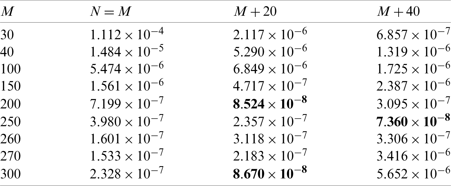
Fig. 5 exhibits  along
along  for the values M = 250 and N = 290. As shown, this error is localized near the bounds of the fixed floating obstacle at x = 0 and at x = W.
Figure 5: The error  for M = 250 and N = 290
The conservation of energy relation (42) associated with the error distribution shown on Fig. 5 is  , with an error of the order of 10−4. while the conservation of mass relation (43) is satisfied identically.
Streamlines are a family of curves that are instantaneously tangent to the velocity vector of the flow. The stream function  assumes constant value on each streamline and the general equation of this family takes the form

where different values of the constant on the R.H.S. of Eq. (62), gives different streamlines.
Fig. 6 illustrates the system of streamlines, in the present application, inside the extended region V.
Figure 6: The system of streamlines inside the control region V
Fig. 7 illustrates the system of streamlines inside the control region V0. The number assigned to each line refers to the constant value of the function  along this line.
Figure 7: The system of streamlines inside the control region V0
The horizontal bottom of the channel is the lowest streamline (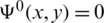 ) and the lower boundary of the fixed floating obstacle is a part of another streamline (
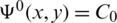 ). For the present application
  .
.
Fig. 7 shows that the fluid particles are accelerated when approaching the fixed floating obstacle.
5.3 Pressure Applied to the Immerged Part of the Fixed Floating Obstacle
The calculation of the dynamical pressure acting on the witted part of the boundary of the fixed floating obstacle (which simulates the floating ship) has a certain practical interest. Fig. 8 illustrates the real part of the dimensionless dynamical pressure along this boundary. The figure shows that the pressure is greater on the side facing the incident wave direction and decreases till attaining its minimum value on the other side.
Figure 8: The dynamical pressure acting on the boundary of the fixed floating obstacle
The objective of the present work is to study a model, simulating the phenomenon of reflection and transmission of an incident wave on a floating ship in a vast ocean. The obtained results may be used in checking the reliability of other methods proposed for studying the same problem. We satisfy exactly the equations and the conditions of the problem except for the condition on the fixed obstacle’s which we satisfy approximately.
The worked applications show that the method is easy to use with reasonable numerical calculations. The accuracy of the method is tested on a particular worked application and the resulting system of streamlines is given and the dynamical pressure acting on the witted part of the surface of the fixed floating obstacle is calculated as well. The limiting case of a floating obstacle having the form of a vertical partially immersed thin barrier needs another procedure for the study and is in progress. This case needs special care.
If the boundary of the floating body contains corner points [25], the solution is singular. This is not physical and comes from the mathematical treatment. To avoid this inconvenient result the corner points should be smoothed to a convenient order.
Funding Statement: The author received no specific funding for this study.
Conflicts of Interest: The author declare that they have no conflicts of interest to report regarding the present study.
1. W. Thomson. (1886). “On stationary waves in flowing water, Part I,” Philosophical Magazine, vol. 5, pp. 353–357. [Google Scholar]
2. W. Thomson. (1887). “On stationary waves in flowing water, Part II,” Philosophical Magazine, vol. 5, pp. 445–452. [Google Scholar]
3. L. Huang, K. Ren, M. Li, Z. Tukovic, P. Cardiff et al. (2019). , “Fluid-structure interaction of a large ice sheet in waves,” Ocean Engineering, vol. 182, pp. 102–111. [Google Scholar]
4. M. Farhat. (2020). “Scattering theory of gravity-flexural waves of floating plates water,” Physical Review B, vol. 101, no. 1, pp. 14307. [Google Scholar]
5. S. H. Lamb. (1994). “Hydrodynamics,” Dover Book on Physics, Sixth Revised ed., New York. [Google Scholar]
6. J. V. Wehausen and E. V. Laitone. (1966). Surface waves Handbuch der Physik, vol. 9. Berlin: Springer. [Google Scholar]
7. M. S. Abou-Dina and M. A. Helal. (1990). “The influence of a submerged obstacle on an incident wave in stratified shallow water,” European Journal of Mechanics - B/Fluids, vol. 9, pp. 545–564. [Google Scholar]
8. M. S. Abou-Dina and M. A. Helal. (1992). “The effect of a fixed barrier on an incident progressive wave in shallow water,” Nuovo Cimento B, vol. 107, pp. 331–344. [Google Scholar]
9. M. S. Abou-Dina and M. A. Helal. (1995). “The effect of a fixed submerged obstacle on an incident wave in stratified shallow water (Mathematical Aspects),” Nuovo Cimento B, vol. 110, pp. 927–942. [Google Scholar]
10. J. J. Xie, H. W. Liu and P. Lin. (2011). “Analytical solution for long-wave reflection by a rectangular obstacle with two scour trenches,” Journal of Engineering Mechanics, vol. 137, pp. 919–930. [Google Scholar]
11. M. S. Abou-Dina. (2001). “Nonlinear transient gravity waves due to an initial free surface elevation over a topography,” Journal of Computational and Applied Mathematics, vol. 130, pp. 173–195. [Google Scholar]
12. C. Hazard. (2015). “On the absence of trapped modes in locally perturbed open waveguides,” IMA Journal of Applied Mathematics, vol. 80, pp. 1049–1062. [Google Scholar]
13. J. T. Kirby. (1986). “A general wave equation for waves over rippled beds,” Journal of Fluid Mechanics, vol. 162, pp. 171–186. [Google Scholar]
14. J. Miles. (1998). “On gravity-wave scattering by non-secular changes in depth,” Journal of Fluid Mechanics, vol. 376, pp. 53–60. [Google Scholar]
15. J. Miles and P. Chamberlain. (1998). “Topographical scattering of gravity waves,” Journal of Fluid Mechanics, vol. 361, pp. 175–188. [Google Scholar]
16. P. F. Rhodes-Robinson. (1996). “On the forced surface waves due to a partially immersed vertical wavemaker in water of infinite depth,” Quarterly of Applied Mathematics, vol. 4, pp. 709–719. [Google Scholar]
17. F. Nelli, L. G. Bennetts, D. M. Skene, J. P. Monty, J. H. Lee et al. (2017). , “Reflection and transmission of regular water waves by a thin floating plate,” Wave Motion Journal, vol. 70, pp. 209–221. [Google Scholar]
18. R. W. Yeung. (1982). “Numerical methods in free-surface flows,” Annual Review of Fluid Mechanics, vol. 14, pp. 395–442. [Google Scholar]
19. J. A. Kolodziej. (1987). “Review of application of boundary collocation methods in mechanics of continuous media,” Mathematics, vol. 12, pp. 187–231. [Google Scholar]
20. A. P. Zielinski and I. Herrera. (1987). “Trefftz method: Fitting boundary conditions,” International Journal for Numerical Methods in Engineering, vol. 24, pp. 871–891. [Google Scholar]
21. A. H. Nayfeh. (1981). Introduction to perturbation techniques. New York: Interscience Pub. [Google Scholar]
22. M. S. Abou-Dina and M. A. Helal. (1998). “Reduction for the nonlinear problem of fluid waves to a system of integro-differential equations with an oceanographical application,” Journal of Computational and Applied Mathematics, vol. 95, pp. 65–81. [Google Scholar]
23. M. S. Abou-Dina and M. A. Helal. (2000). “Boundary integral method applied to the transient nonlinear wave propagation in fluid with initial free surface elevation,” Applied Mathematical Modelling, vol. 24, pp. 535–549. [Google Scholar]
24. G. Fairweather and A. Karageorghis. (1998). “The method of fundamental solutions for elliptic boundary value problems,” Advances in Computational Mathematics, vol. 9, pp. 69–95. [Google Scholar]
25. M. S. Abou-Dina and F. M. Hassan. (2005). “Approximate determination of the transmission and reflection coefficients for water-wave flow over a topography,” Applied Mathematics and Computation, vol. 168, pp. 283–304. [Google Scholar]
26. A. Abbasnia and M. Ghiasi. (2014). “Simulation of irregular waves over submerged obstacle on a NURBS potential numerical wave tank,” Latin American Journal of Solids and Structures, vol. 11, pp. 2308–2332.
27. M. S. Abou-Dina and A. F. Ghaleb. (2016). “Multiple wave scattering by submerged obstacles in an infinite channel of finite depth I. Streamlines,” European Journal of Mechanics - B/Fluids, vol. 59, pp. 37–51. [Google Scholar]
28. L. G. Bennetts and T. D. Williams. (2015). “Water wave transmission by an array of floating discs,” Proceedings of the Royal Society of London: Series A, vol. 471, pp. 20140698. [Google Scholar]
29. W. W. Ding, Z. J. Zou, J. P. Wu and B. G. Huang. (2019). “Investigation of surface piercing fixed structures with different shapes for Bragg reflection of water waves,” International Journal of Naval Architecture and Ocean Engineering, vol. 11, pp. 819–827. [Google Scholar]
30. N. Drimer, Y. Agnon and M. Stiassnie. (1992). “A simplified analytical model for a floating breakwater in water of finite depth,” Applied Ocean Research, vol. 14, pp. 33–41.
31. N. Kuznetsov and O. Motygin. (2012). “On the coupled time-harmonic motion of deep water and a freely floating body: Trapped modes and uniqueness theorems,” Journal of Fluid Mechanics, vol. 703, pp. 142–162.
32. B. N. Mandal. (2006). “Water wave scattering by bottom undulations in the presence of a thin partially immersed barrier,” Applied Ocean Research, vol. 28, pp. 113–119.
33. P. A. Martin. (2006). “Multiple scattering, interaction of time-harmonic waves with N obstacles. bridge University Press, Corrections, and addition.
34. F. Montiel, L. G. Bennetts, V. A. Squire, F. Bonnefoy and P. Ferrant. (2013). “Hydroelastic response of floating elastic disks to regular waves. Part 2: Modal analysis,” Journal of Fluid Mechanics, vol. 723, pp. 604–628. [Google Scholar]
35. W. Peng, K. H. Lee, S. H. Shin and N. Mizutani. (2013). “Numerical simulation of interaction between water wave and inclined-moored submerged floating breakwaters,” Coastal Engineering, vol. 82, pp. 76–87. [Google Scholar]
36. R. Shih, C. Chou and J. Yim. (2005). “Numerical estimation of wave reflection coefficients for irregular waves over submerged obstacles,” International Journal of Offshore and Polar Engineering, vol. 246, pp. 19–24. [Google Scholar]
37. P. J. Cobelli, V. Pagneux, A. Maurel and P. Petitjeans. (2011). “Experimental study on water-wave trapped modes,” Journal of Fluid Mechanics, vol. 666, pp. 445–476. [Google Scholar]
38. A. S. Koram and O. S. Rageh. (2013). “Effect of under connected plates on the Hydrodynamic efficiency of the floating breakwater,” China Ocean Engineering, vol. 28, pp. 349–362. [Google Scholar]
39. O. S. Ragih, K. S. El-Alfy, M. T. Shamaa and R. M. Diad. (2006). An Experimental Study of Spherical Floating Bodies Under Waves. Egypt: IWTC10, pp. 357–375. [Google Scholar]
40. D. M. Skene, L. G. Bennetts, M. H. Meylan and A. Toffoli. (2015). “Modelling water wave over wash of a thin floating plate,” Journal of Fluid Mechanics, vol. 777, pp. 1–13. [Google Scholar]
41. Y. Yu, Z. Guo and Q. Ma. (2018). “Transmission of water waves under multiple vertical thin plates,” Water, vol. 10, pp. 517. [Google Scholar]
42. C. J. Tranter. (1966). Integral Transforms in Mathematical Physics. 3rd ed., London: Methuen Co. Ltd. [Google Scholar]
 | This work is licensed under a Creative Commons Attribution 4.0 International License, which permits unrestricted use, distribution, and reproduction in any medium, provided the original work is properly cited. |
