DOI:10.32604/cmc.2021.015250
| Computers, Materials & Continua DOI:10.32604/cmc.2021.015250 | |
| Article |
Analyzing Some Elements of Technological Singularity Using Regression Methods
1Department of Electrical and Computer Engineering, University of Delaware, Newark, DE, 19716, USA
2Department of Computer Science, Purdue University, West Lafayette, IN, 47907, USA
*Corresponding Author: Ishaani Priyadarshini. Email: ishaani@udel.edu
Received: 12 November 2020; Accepted: 02 January 2021
Abstract: Technological advancement has contributed immensely to human life and society. Technologies like industrial robots, artificial intelligence, and machine learning are advancing at a rapid pace. While the evolution of Artificial Intelligence has contributed significantly to the development of personal assistants, automated drones, smart home devices, etc., it has also raised questions about the much-anticipated point in the future where machines may develop intelligence that may be equal to or greater than humans, a term that is popularly known as Technological Singularity. Although technological singularity promises great benefits, past research works on Artificial Intelligence (AI) systems going rogue highlight the downside of Technological Singularity and assert that it may lead to catastrophic effects. Thus, there is a need to identify factors that contribute to technological advancement and may ultimately lead to Technological Singularity in the future. In this paper, we identify factors such as Number of scientific publications in Artificial Intelligence, Number of scientific publications in Machine Learning, Dynamic RAM (Random Access Memory) Price, Number of Transistors, and Speed of Computers’ Processors, and analyze their effects on Technological Singularity using Regression methods (Multiple Linear Regression and Simple Linear Regression). The predictive ability of the models has been validated using PRESS and k-fold cross-validation. Our study shows that academic advancement in AI and ML and Dynamic RAM prices contribute significantly to Technological Singularity. Investigating the factors would help researchers and industry experts comprehend what leads to Technological Singularity and, if needed, how to prevent undesirable outcomes.
Keywords: Technological growth; technological singularity; regression analysis; artificial intelligence; superintelligence; PRESS; k-fold validation
Over the last few years, technology has impacted several industries, like medicines, computing, power systems, automobiles, etc. The field of artificial intelligence has significantly led to systems getting smarter and making human lives easy. Intelligent systems are machines with embedded, Internet-connected computers capable of gathering and analyzing data to communicate with other systems. Advancement in technology has led to the emergence of systems like personal assistants, automated drones, smartphones, video games, smart homes, etc. Many of these are not only confined to carrying out tasks but are also capable of interacting with humans [1–3]. Conversational marketing bots, manufacturing robots, and smart assistants have decision-making capabilities and have already started replacing humans in several sectors [4,5]. The quest for a comfortable life encourages humans to train systems to make them as intelligent as possible to assist humans in making their jobs easier. Many researchers and industry experts welcome the idea of making machines as intelligent as possible. Other subject matter experts and visionaries see this as a threat. While human intelligence is limited, machine intelligence might not be. Artificial Intelligence has made significant progress in various fields, and can outsmart humans in games [6], identify images better [7], pass Turing tests [8], etc. The very early signs of machine intelligence leading to undesirable outcomes were seen in Twitter bots making insensitive comments [9], systems making racial discrimination [10], self-driving cars having deadly accidents [11], and patrol robots colliding with a child [12]. According to several researchers, there may come the point when machine intelligence becomes equal to that of humans or surpasses it by a considerable margin, a term they label as Technological Singularity [13,14]. Technological Singularity is a hypothetical future point in which technological growth becomes uncontrollable and irreversible. Such a situation may result in unforeseeable changes to human civilization, attributed to the rate at which technological advancements occur. An entity or a system possessing such a level of intelligence may be termed as super intelligent. Recent studies show that machines are getting better than humans in several games, making predictions and imitating humans as smart assistants. All these features hint towards better machines’ capabilities than humans. Reference [15] describe Technological Singularity as a point of no return. Such a situation may be synonymous with the term ‘Event Horizon’ for machine intelligence, which defines the boundary marking the limits of human intelligence. Thus, human intelligence may eventually be surpassed by machines. Several researchers in the past have tried to validate the possibility of technological singularity in the future. While machines gaining superintelligence can make lives easy, many researchers argue that machine superintelligence could also pose a threat to human lives. Apart from succumbing to economic collapse and losing jobs, there are several other reasons to fear Technological Singularity. Technological singularity may lead to environmental catastrophe and loss of humanity, and also a global apocalypse. Artificial intelligence systems that go rogue, provide a glimpse of such a situation, although on a smaller scale [16]. Although there is no concrete evidence of the risks and the risk levels associated with Technological Singularity, the concept cannot be pushed entirely aside [17]. Thus, there is a need to analyze the hypothesis in detail and list certain factors that lead to Technological Singularity. This paper lists some quantitative factors that could lead to technological advancement; hence, it may also affect Technological Singularity. Technological Advancement is driven by dynamic industry and flourishing academia. Therefore, Technological Singularity can find its factors in both these realms. Since the industry is motivated by academia, published work can be considered an essential element for technological advancement. Therefore, we consider publications in Machine Learning and Artificial Intelligence as significant parameters for the study. Moreover, for carrying out most of the computations, we rely on the speed of computers, the number of transistors, and sometimes the Dynamic RAM (Random Access Memory). Changes in these factors’ values over time can give us a clear idea about technological advancement, and hence these factors may be contributors to Technological Singularity. These factors find their basis in Moore’s Law, which states that a computer’s speed can be expected to double every two years if the number of transistors on a microchip are increased. We rely on regression methods to analyze the effects of these factors on technological progress. The key contributions of this paper are as follows:
a) There is limited research on Technological Singularity. We attempt to explore the domain in yet another way. We identify some factors that can contribute to Technological Singularity.
b) Most of the research works conducted in the past concerning Technological Singularity consider Technological Singularity as a concept or hypothesis, due to which neither experiments nor quantified results are involved for interpretation. In this paper, we perform an in-depth analysis of the factors considered by using regression methods. We determine three models (equations)
— One Multiple Linear Regression (MLR) model using three factors, i.e., Number of scientific publications in Artificial Intelligence, Number of scientific publications in Machine Learning, and Dynamic RAM (Random Access Memory) Price.
— Two Simple Linear Regression (SLR) models using one factor each, i.e., Number of Transistors, and Speed of Computers’ Processors
The validation has been performed using the PRESS (predicted residual error sum of squares) and k-fold cross-validation.
The study also finds solutions for the derived equations.
The rest of the paper is organized as follows. Section 2 describes materials and methods. In this section, we list out some related works that have been done in the past and our proposed work. In Section 3, we discuss the experimental analysis. Section 4 discusses the Results. This section also includes performance evaluation and validation. In Section 5, we present the conclusions and future work.
This section has been divided into two subsections. The first subsection lists some of the related works done in the past on the technological singularity. In the second section, we present several factors that can lead to Technological Advancement and hence may be related to Technological Singularity.
A study [13] observed technological progress’s acceleration and argued that technology might create entities that have intelligence greater than humans. Superintelligence may be achieved through several means like intelligent computers, extensive networks, computer-human interfaces, biomedical domain, and digital means. In [18], the authors performed a study to identify trends showing technological advancement growth. In his research, Kurzweil identified trends concerning cell phone users over time, inventions over time, development of computing over time, internet hosts over time, DNA (Deoxyribonucleic Acid) sequence data, etc., as contributors to the technological singularity. Another study [19] presented technological singularity as exponential technological advancement. Exponential growth for input and output mechanisms of a sensory system and response time are considered for the study. The measures of comparative intelligence were analyzed in terms of change in entropy or state change. Likewise, a survey [20] highlights past research works on Technological Singularity compared to the works of Kurzweil [18] and Moore [21]. A combination of processing power and contextual knowledge could very well lead to the technological singularity. The post-singularity era may pose significant challenges for human beings to determine their role in society. There is a need to think about ways to control machines that turn malevolent. Reference [22] proposed the conditions necessary for computer simulations as a way of achieving technological singularity. Enhancement of the computer-human cognitive capabilities and the reliability of computer simulations have been considered for the study. In [23], the authors presented an updated overall idea about technological singularity and the possibility of creating artificial general intelligence. Metasystem transitions and universal evolution are considered for making some observations. The study discusses timeline extrapolation as one of the techniques for making predictions along with some possible scenarios. Reference [24] presented research contradicting the projections made by [25], which asserted that Technological Singularity might never happen. Yampolskiy opposed Walsh’s arguments based on specific statements. Some of these arguments are: the speed alone does not bring intelligence, human intelligence is not exceptional, many fundamental limits exist within the universe, and no growth in performance will make undecidable problems decidable. Likewise, a study was conducted [26] to highlight artificial consciousness’s importance to reach Technological Singularity. The study mentions that artificial consciousness underpinning the concepts, sophisticated algorithms of learning, and machine discovery can lead to Technological Singularity. Moreover, [27] presented a study on technological singularity based on search for extraterrestrial intelligence. The argument is based on a specific scenario of whether intelligent life happens to be a normal phenomenon in the Milky Way Galaxy. Moreover, suppose the rate of technological evolution is at least as advanced as that on Earth. In that case, there is a possibility that the Milky Way Galaxy must be full of highly developed technological civilizations. It might also be possible for us to see them, and they could also be here, but we do not see them, which may be attributed to the Fermi paradox. In [28], the authors presented the concept of cyber singularity concerning intelligence being observed in Cyberspace. Many past research works suggest different ways of achieving Technological Singularity. Some of these research works contemplate Technological Singularity as a concept or hypothesis. Therefore, several research papers lack interpretation involving the experimental analysis and quantified results. While the field is mostly unexplored, many researchers also believe that it may never happen [29]. There is a need to explore the area by performing extensive analysis. In the next section, we shall discuss the proposed work.
Technological Singularity deals with machines gaining intelligence equal to or more than humans; artificial intelligence underpinning machine learning concepts, natural language processing, deep learning, machine memory, etc. [30–33]. The pace with which technological advancement is moving may affect Technological Singularity. Therefore, it is essential to discuss what factors contribute to the same. In this section, we identify some factors that may affect Technological Singularity. We will analyze these factors using Regression Methods in the later areas. The following are the factors that have been considered for the study.
a) The number of scientific publications in Artificial Intelligence: Scientific journals intend to advance science’s progress by reporting new research. Since technology is significantly driven by artificial intelligence these days, the number of scientific publications may impact technological advancement and may be considered a driver for technological singularity.
b) The number of scientific publications in Machine Learning: The most popular subdomain of artificial intelligence is machine learning. The study of algorithms and statistical models to perform a specific task without being explicitly programmed is one way to create intelligent machines. As machine learning gets better, systems may get more intelligent, and there may come a time when system intelligence surpasses that of humans.
c) Dynamic RAM Price: Dynamic RAM is a random-access semiconductor memory that stores each bit of data in a memory cell consisting of a tiny capacitor and a transistor. The Dynamic RAM price (bits per dollar, at production) has been increasing over the last few decades, indicating an increase in DRAM speeds. Therefore, it may be asserted that processing power and memory capacity have been growing.
d) Number of Transistors: Speed of computing may have an impact on Technological Advancement. With more transistors in a given chip, the speed of computing increases. Moore’s Law states that the number of transistors on a microchip doubles every two years, though the cost is halved. Thus, we can expect our computers’ speed and capability to increase every couple of years and pay less for them.
e) Speed of Computers’ Processors: Processing speed determines the performance of computing devices. Better the performance of computing devices rapidly would be technological advancement. Million Instructions Per Second (MIPS) measures the raw speed of a computer’s processor. Processing speed may have an impact on the performance of computing devices, which directly impacts technological advancement.
This section discusses the datasets essential for our study and the experimental methods adopted to justify our research work.
Since our research work deals with regression analysis of the proposed factors, the data was taken from reliable sources. The datasets for the number of transistors and speed of computer processors have been taken from the data repository ‘Our World in Data by,’ Technological Progress by The Oxford University (https://ourworldindata.org/technological-progress) [34]. The Dynamic RAM price data has been taken from http://www.singularity.com/charts/page58.html [35]. The website is based on Kurzweil’s idea of technological singularity. Although there are several factors listed that may lead to technological advancement, we chose the Number of Transistors, Speed of Computer Processors, and Dynamic RAM [36] because the data is recent from the list of factors mentioned. There were enough data points to conduct the analysis, unlike any other factors mentioned on the respective websites. The study finds its basis in Moore’s Law. The number of Artificial Intelligence and Machine Learning publications has been taken from the National Center for Biotechnology Information (NCBI) PubMed. The number of research papers until March 31, 2020, has been considered. The analysis has been conducted using the R programming language (R Studio). We perform Multiple Linear Regression considering the Number of publications for Artificial Intelligence and Machine Learning and Dynamic RAM price. Owing to the lack of abundant data points, microprocessors, and processing speed (MIPS) have been analyzed using Simple Linear Regression. The solution space for the three equations has been plotted using MATLAB.
We have already identified a list of factors that may contribute to Technological Singularity. We intend to introduce the factors mentioned in the previous section as variables for two family equations. These factors’ effects on technological singularity will be analyzed using regression methods [37,38]. Since the data pertaining to the five factors listed in the previous section is sparse, we conduct the analysis using two families of equations. The first equation incorporates the elements Number of Artificial Intelligence Publications, Number of Machine Learning Publications, and Dynamic RAM Price (bits per dollar). The second equation includes the factors. To conduct the analysis, we perform the following steps using statistical language R. The ALSM package, which is Companion to Applied Linear Statistical Models, has also been relied on to perform the analysis.
While there is enough data to conduct Multiple Linear Regression (MLR) with a number of publications for Artificial Intelligence and Machine Learning, and Dynamic RAM price due to sufficient data, there is not enough data to conduct MLR for transistors and MIPS. Therefore, transistors and MIPS have been analyzed using Simple Linear Regression, a particular case of MLR. We will here be considering first-order models.
Multiple Linear Regression: Multiple regression generally explains the relationship between multiple independent or predictor variables and one dependent or criterion variable. A dependent variable is modeled as a function of several independent variables with corresponding coefficients and the constant terms. Multiple regression requires two or more predictor variables, and this is why it is called multiple regression. The multiple regression equation explained above takes the following form:


In Eq. (1), Y represents the actual/true prediction.  ’s (
’s ( ) represent the Population Parameters.
  is the random error associated with that prediction such that
  , such that N represents normal distribution and
  denotes population variance. Additionally, they are identically and identically distributed.
In Eq. (2),  is the point estimate or the best predictive value. bi’s (
 ) are the regression coefficients (also known as sample statistic), representing the value at which the criterion variable changes when the predictor variable changes, b0 intercept.
Our goal is to mimic the behavior of Eq. (1) using Eq. (2). Here,  , p referring to the number of parameters. The number of parameters (p) is given by the Number of predictors (q)+1 (for first-order models), where n stands for the number of rows/instances/tuples in the dataset. Hence,
  ;
;  and
and  and
and  , where
  and s
and s . Here, s denotes sample standard deviation, q denotes the number of predictors, and s2 depicts sample variance. For conducting the analysis, we need to make the following assumptions:
a) Explanatory variable and response variable(s) follow a linear relation.
b) Residuals ( ) are independently identical.
c) Residuals follow a Normal Distribution.
d) Residuals have constant variance.
The following steps have been considered for conducting the analysis:
a) Linearity Test: Before performing a linear regression analysis, we test our data for linearity. Linearity means that two variables, x, and y are related by a mathematical equation y = cx, where c is any constant number. A linear graph indicates a steady-state increase.
b) Histogram: The datasets used for the research are univariate data sets, i.e., they have one variable. The purpose of a histogram is to summarize the distribution of a univariate data set graphically.
c) Transformation using Log Histogram: To respond to the skewness of large values, a histogram based on the logarithmic scale may be used. If one or a few points are much larger than the bulk of data, log histograms may be used for analysis.
d) Transformation using Box-Cox: A Box-Cox transformation is a way to transform non-normal dependent variables into a standard shape. Normality is an essential assumption for many statistical techniques. If the data is not standard, applying a Box-Cox enables running a broader number of tests. We perform Box-Cox transformation using the Maximum Likelihood (MLE). The range chosen to select lambda was ( −10, 10). New transformed 
e) Independently Identical Distribution: When the no. of observations (n) is less than  (p is the number of parameters), the errors are said to be dependent on one another. Hence, a good generalization needs to be made. Therefore,
  is a good rule of thumb to follow [39]. No apparent pattern in residual plots also signals the same. Pearson Residuals can determine the model fit. A residual is a difference between the observed y-value (from scatter plot) and the predicted y-value (from the regression equation line).
f) Shapiro Wilk Normality Test: The Shapiro–Wilk test is a test for normal distribution exhibiting high power. It may lead to good results, even with a small number of observations. It is only applicable to check for normality. The basic idea behind the Shapiro–Wilk test is to estimate the variance of the sample in two ways. Firstly, the regression line in the QQ-Plot (probability plot) allows estimating the variance. Secondly, the variance of the sample can also be regarded as an estimator of the population variance. Both estimated values should approximately be equal in the case of a normal distribution and thus should result in a quotient close to 1. If the quotient is significantly lower than 1.0, then the null hypothesis (of having a normal distribution) should be rejected.
g) Brown–Forsythe test: The Brown–Forsythe (B–F) Test is for testing the assumption of equal variances in the Analysis of variance (ANOVA). The Brown-Forsythe test attempts to correct for this skewness by using deviations from group medians. The result is a more robust test. This test does not consist of dividing by the mean square of the error. Instead, the mean square is calibrated using the observed variances of each group. The underlying idea is not to assume that all populations are normally distributed. It is performed when the normality assumption is not viable.
h) Regression Influence Plot: The influence plot helps identify individual data points that might have undue influence over the fitted regression equation. Unusual data points can be unusual because they have an unusual combination of X values, or their Y value is given their X values. Points with usual Xs may be defined as high-leverage points, and points with unusual Y values (given X) are termed outliers.
i) Ridge Regression: Ridge Regression is a technique for analyzing multiple regression data that suffer from multicollinearity. Variance Inflation Factor (VIF) detects multicollinearity in regression analysis. When multicollinearity occurs, least squares estimates are unbiased, but their variances are large, so they may be far from the true value. By adding a degree of bias to the regression estimates, ridge regression reduces the standard errors.
j) R-square-coefficient: In regression, the R square coefficient of determination is a statistical measure of how well the regression predictions approximate the real data points. An R square of 1 indicates that the regression predictions perfectly fit the data.
k) P-Value: P-value helps to determine the significance of results. A small p-value (typically  0.05) indicates strong evidence against the null hypothesis, so the null hypothesis is rejected.
l) W-Value: W value is associated with the Shapiro–Wilk Normality Test. The test gives a W value; small values indicate that the sample is not normally distributed (it is acceptable to reject the null hypothesis that the population is normally distributed if the values are under a certain threshold).
m) Type 1 error,  for all testing and analysis. The probability of making a type I error is represented by alpha level (
 ), which is the p-value below which the null hypothesis is rejected.
The following figure is an illustration of the analysis conducted by us (Fig. 1).
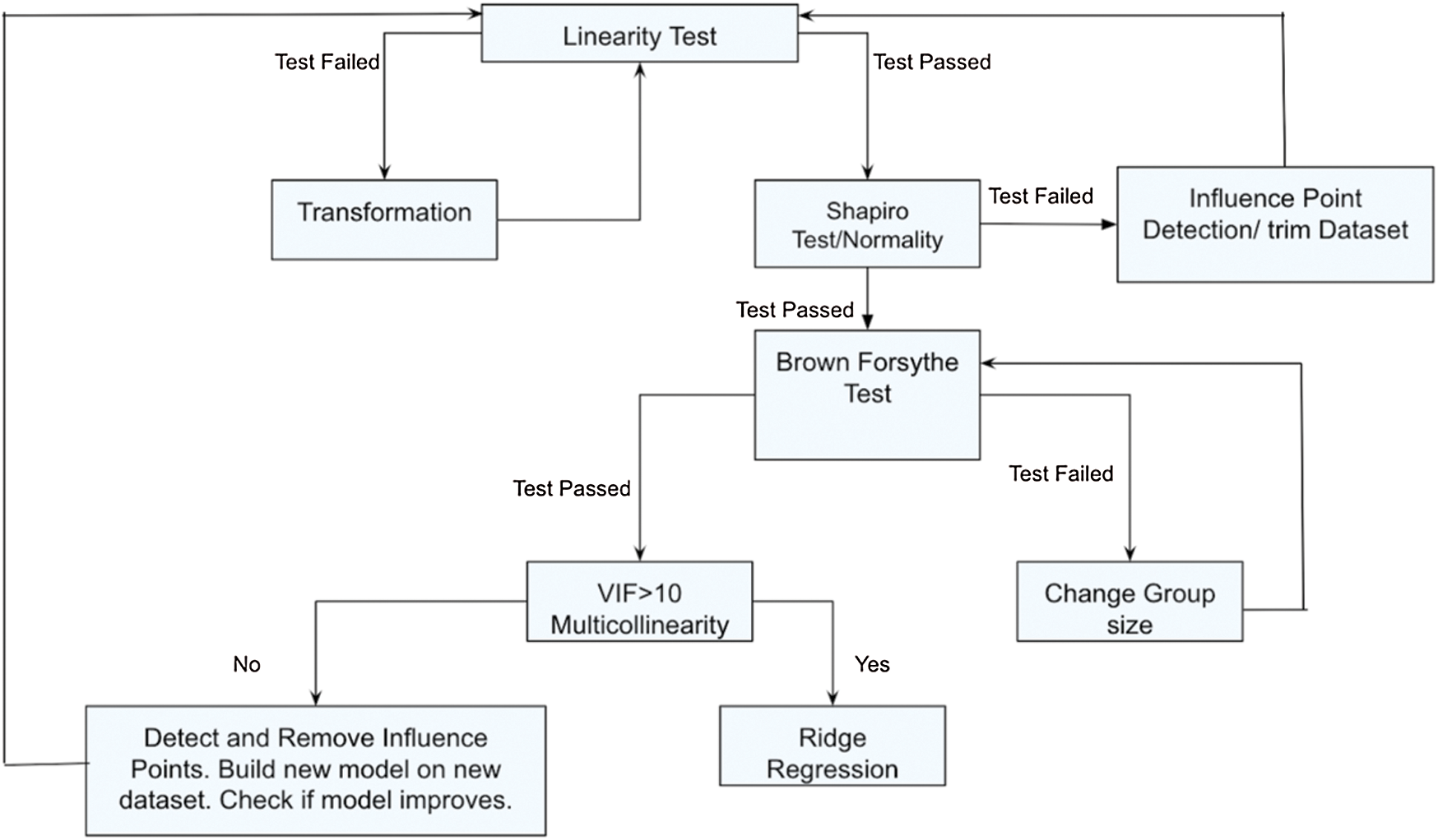
Figure 1: Steps for the analysis conducted
Although the Variance Inflation Factor (VIF) detects multicollinearity, multicollinearity does not make sense if there is one variable.
The analysis conducted may be explained in the following steps:
— Step 1: Check for Linearity Test — Step 2: If Test Failed, proceed to Transformation and eventually conduct Linearity Test + If Test Passes, perform Shapiro Test, check Normality.
— Step 3: If Test Failed, perform Influence Point Detection/Trim dataset and conduct Linearity Test + If Test Passes, perform Brown Forsythe Test
— Step 4: If Test Failed, Change Group size and again perform Brown Forsythe test + If Test Passed, check if Variance Inflation Factor ( ) or Multicollinearity
— Step 5: If there is no multicollinearity, detect, and remove influence points. Build a model on a new dataset and check if the model improves. + If there is multicollinearity, perform Ridge regression.
In this section, we will be discussing the equations, analyzing the model by inspecting the validity of the model, and finding the solution to the equations. We also perform a comparative analysis concerning some previous works that have been done regarding Technological Singularity.
Based on the factors considered and the analysis conducted, we have identified three equations. The first equation has factors like the number of publications in ML, the number of publications in AI, and Dynamic RAM price, which is analyzed using Multiple Linear Regression. The second equation considers the number of microprocessor transistors and has been analyzed using Simple Linear Regression. Finally, the third equation considers Million Instructions Per Second (MIPS) and is analyzed using Simple Linear Regression. The equations are depicted as follows:
a) Eq. (1): 
b) Eq. (2): Y
c) Eq. (3): Y
To perform validation, we rely on two popular methods, i.e., PRESS statistic and k-fold cross-validation.
PRESS refers to the predicted residual error sum of squares. This statistic is a form of cross-validation used in regression analysis for providing a summary measure of the fit of a model to a sample of observations that were not themselves used to estimate the model. It is given by the summation of squares of the prediction residuals for those observations.

The lowest values of PRESS indicate the best structures. If a model is overfitted, small residuals for observations will be included in the model-fitting, but large residuals for observations will be excluded. Thus, the smaller the PRESS value, the better the model’s predictive ability.
For Eq. (1),

The slopes are unknown to accompany bias due to shrinkage. Hence, the prediction would not be accurate; rather, it would not be viable to compute the Y values based on these biased values. However, the low Akaike Information Criterion (AIC) value is indicative of a good prediction. The AIC values are used for estimating the likelihood of a model for predicting/estimating future values. The best model has the minimum AIC value among all other models. Hence it provides a means for model selection. Also, the model explains 92.47% of the variance in Y, which is reasonably good. The Bayesian Information Criterion (BIC) is closely related to AIC. Adding parameters for model fitting may often lead to overfitting. BIC resolves this by introducing a penalty term for the number of parameters in the model. The BIC value is not as low as AIC, but this value implies that our model may not be the most parsimonious.
We observe that the Mean Square Error (MSE) is also high, with a value of 1451.15. Hence, the model parameters are relevant. However, using the predicted residual error sum of squares (PRESS), we observe that the value of K increases with K increasing from 0 to 0.11 and beyond (Fig. 2).
Fig. 2 depicts the PRESS vs. Predictor Values. As we know, the smaller the PRESS value, the better the model’s predictive ability.
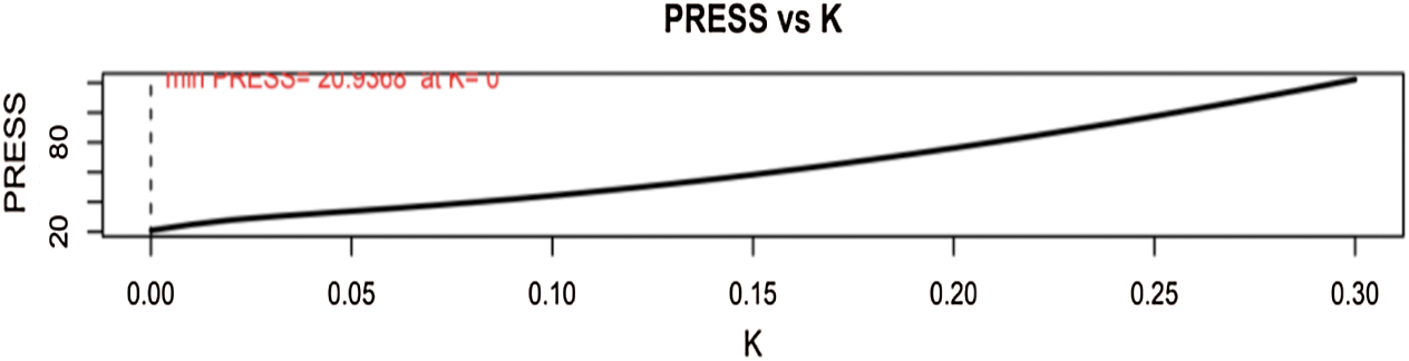
Figure 2: PRESS vs. predictor values (K)
From Fig. 3, it is evident that at ( ), the value of PRESS is 46.4213.
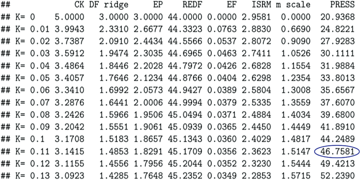
Figure 3: PRESS values for Eq. (1)
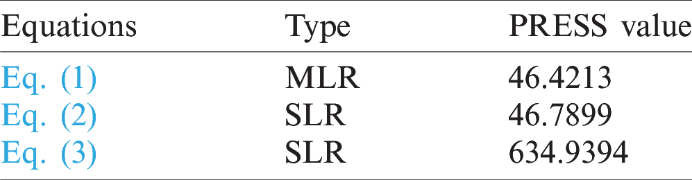
Tab. 1 depicts the PRESS values for all three equations. While PRESS values for Eqs. (1) and (2) are 46.4213 and 46.7899, respectively, the PRESS value for Eq. (3) is 634.9334. Since the lowest PRESS values indicate the best structures, Eq. (1) has the best model predictive ability.
Table 1: PRESS values for the equations
Due to multicollinearity in Eq. (1), we performed Ridge Regression. This led to the introduction of bias in the slopes. Although we initially assumed normal distribution, the introduced arbitrary bias does not give much information on the sampling distribution. Hence, statistical inference corresponding to a confidence interval and hypothesis testing will not hold. To evaluate the likely range of values for our population mean, we calculate the confidence interval. Confidence intervals are used for measuring the degree of uncertainty or certainty in a sampling method. The confidence interval with 95% confidence has been calculated as follows:
CI = Point Estimate  Margin of Error
Margin of Error = Standard Error  t(1 − (
 ), n − p), where t is the critical value given by the software (R studio)
For Eq. (2),
CI for b0 with 95% confidence: −31.81850  1.10115
  t (0.975,23 − 2)
=(29.528, 34.108), where b0 is the intercept
CI for b1 with 95% confidence: 4.28581  0.06238
  t(0.975,23 − 2)
=(4.156, 4.415), where b1 is the slope
For Eq. (3),
CI for b0 with 95% confidence:
12.1780  1.5477
  t(0.975,23 − 2)
=(8.959, 15.396), where b0 is the intercept
CI for b1 with 95% confidence: −3.9230  0.2436
  t(0.975, 23 − 2)
=(−4.429, −3.416), where b1 is the slope
4.2.2 Validation Using K-Fold Cross-Validation
Cross-validation is a resampling procedure used for evaluating machine learning models on a limited data sample. K refers to the number of groups that a given data sample is to be split into. In k-fold cross-validation, the available dataset is partitioned into k number of disjoint subsets, which are of equal size. The number of resulting subsets is known as folds. The partitioning is done by randomly sampling the dataset without any replacement.  subsets denote the training set, and the remaining subset is referred to as the validation set. The performance of each of the subsets is measured until k subsets have served as validation sets. Finally, the average of the performance measurements on the k validation is determined as the cross-validated performance.
To validate the models, we perform the k-fold validation and also observe the values for
Eq. (1): Performing k-Fold validation, where (k = 5)
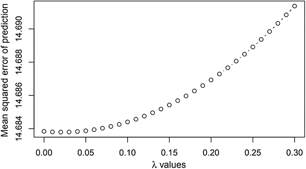
Figure 4: MSPE vs. 
Fig. 4 depicts the plot between the Mean squared error of prediction (MSPE) vs.  , a vector with a grid of values of
  to be used. The values on the MSPE axis are 14.884, 14.686, 14.688, 14.690, and so on. The values on the
  axis are 0.00, 0.05, 0.10, 0.15, and so on. We observe that when
  , the values for MSPE lie between 14.684 and 14.686.
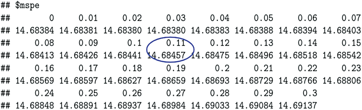
Figure 5: MSPE values
The Mean Square Percentage Error (MSPE) is based on the value of k. From Fig. 5,  , for
, for  .
.
Root Mean Square Percentage  , hence
We directly compute the RMSPE over the validation data and get the percentage error.
Eq. (2): Performing k-Fold validation, where (k = 5)
The validation metrics used for Eq. (2) are depicted in Fig. 6. We observe that the RMSE value is 1.406764, and the Mean Absolute Error (MAE) is 1.235215.

Figure 6: Validation metrics for Eq. (2)
Eq. (3): Performing k-Fold validation, where (k = 5)
Similarly, the validation metrics used for Eq. (3) are depicted in Fig. 7. We observe that the RMSE value is 5.548162, and the Mean Absolute Error (MAE) is 4.606564.

Figure 7: Validation metrics for Eq. (3)
MSE measures the average/mean squared error of our predictions. RMSE Root Mean Square Error is very similar to MSE. MSPE measures the mean square percentage error. MSPE summarizes the predictive ability of a model. RMPSE is the Square Root of MSPE. The variation in Validation means RMPSE for Eq. (1) and RMSE for Eqs. (2) and (3) is strictly due to the ridge summary and summary tables created by the software (R-studio).
4.2.3 Solution to the Equations
Kurzweil’s foresight of the technological Singularity predicts its occurrence in 2045 [11], whereas according to Vinge, Technological Singularity should happen sometime between 2005 and 2030 [6]. The three equations derived consider five factors that we have identified, and all these equations can give some information about when Technological Singularity might happen. In this section, we try to find a solution to the equations stated previously. For each equation, we present two solutions, first between the years 2005–2030 [13] and for the year 2045 [18]
a) Eq. (1): 
For years: 2005–2030

 ,
,  ,
, 
Denote ln(AI) by X, ln(ML) by Y and ln(RAM) by Z

 ;
;  ;
; 
The above linear inequality may be expressed in a three-dimensional solution space. The solution space for the above equation may be depicted as follows (Fig. 8). The colored region lies in the solution space of the equation derived.
For years: 2045


Denote ln(AI) by X, ln(ML) by Y and ln(RAM) by Z
 ,
,  ,
,  ,
,

 ;
;  ;
; 
The above linear inequality may be expressed in a three-dimensional solution space. The colored region lies in the solution space of the equation derived. The solution space for the above equation may be depicted as follows (Fig. 9).
b) Eq. (2): Y1.1 = −31.81850+4.28581(lx)
For years: 2005–2030


This implies, e (back transform, due to initial log transformation)
Hence, 
For year: 2045


e (back transform, due to initial log transformation)

c) Eq. (3): Y1.1 = 12.1780 −3.9230 (lx)
For Years: 2005–2030


Also, 
This implies,
e (back transform, due to initial log transformation)
Hence, 
For year: 2045


 (back transform, due to initial log transformation)

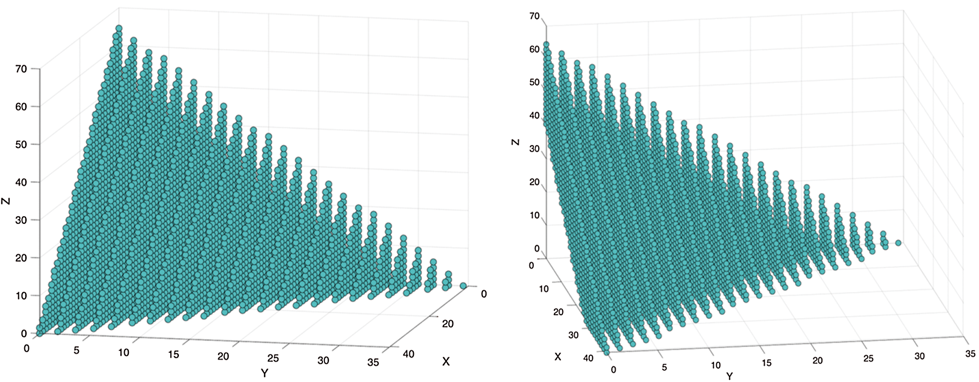
Figure 8: Solution space for Eq. (1) (2005–2030)
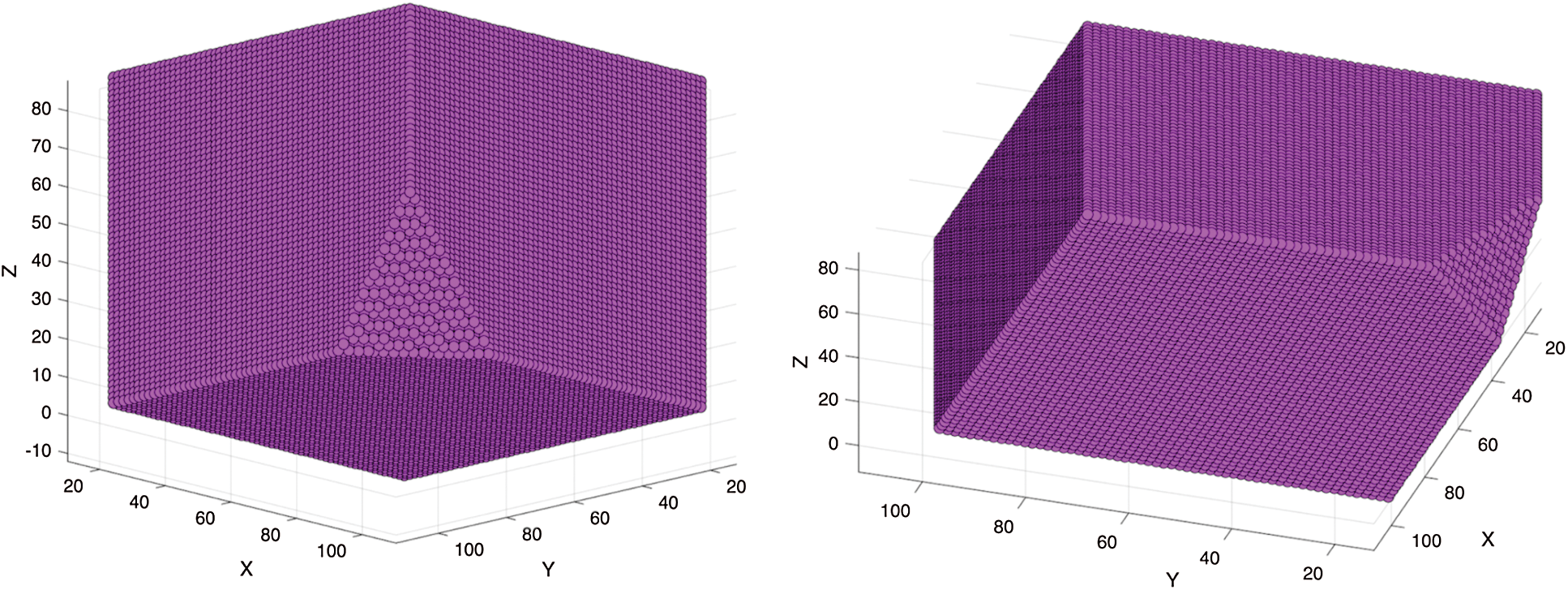
Figure 9: Solution Space for Eq. (1) (2045)
In this section, we present a comparative analysis of our research work concerning some previous research works. Tab. 2 compares our proposed work with previous works in terms of the achieved results.
Table 2: Comparative Analysis of our proposed work

In this study, we identified three equations, which are regression models supporting our research.
Based on the analysis conducted, we can say that Model 1 (Eq. (1), MLR) performs the best, or is the best indicator of Technological Singularity followed by Model 2 (Eq. (2), SLR) and Model 3 (Eq. (3), SLR), respectively. The decision may be attributed to the following factors:
a) PRESS value: Comparing the PRESS values for the equations (models), we find that the PRESS value for model 1 is the least followed by models 2 and 3, respectively. As we know, the smaller the PRESS value, the better the model’s predictive ability. Hence Model 1’s predictive ability is the best.
b) The solution space for Model 1 is represented in a three-dimensional space. Comparing the solutions for Model 2 and Model 3, we find that the solutions for Model 3 are too small concerning the other models, which verifies our judgment of Model 3 being the least suitable.
c) The RMSE and RMSPE values, as evaluation criteria, indicate that the performance of Model 1 and Model 2 is significantly better than Model 3.
Some Limitations of the study are as follows:
a) The predictor variable is treated as being continuous. It is hard to infer what a real-valued prediction means. Hence, predictions must be reported with Confidence Intervals (Mean Response or Single Response).
b) Model 1 was treated using Ridge Regression, i.e., variables less significant were shrunk to a greater extent than the more significant variables. This is known to induce bias in the model. MSE, as large as 1451.15, is indicative of that. The BIC value is not as low, but this value implies that our model may not be the most parsimonious model.
c) Consider Model 1,

d) Mathematically, when  , this implies
  . In other words, our model guarantees that Technological Singularity is to happen after 1965–1966, which is a very strong assumption to make.
e) Additionally, the study has been carried out using the R-programming language, which has some limitations of its own. R utilizes more memory. Hence it is not ideal for handling big data. The packages and the programming language confined to R are relatively slow. Moreover, the algorithms are spread across packages, which is challenging as well as time-consuming.
The fascinating field of Artificial Intelligence promises innovations and advancement in multiple realms of technology. However, it also brings the anticipation of an unseen tomorrow, which may witness machines gaining intelligence greater than or equal to humans, and the society does not entirely benefit from it. Hence, there is a need to identify specific factors that may contribute to this technology advancement so that appropriate measures may be taken if such a situation arises. This paper identified additional factors that can lead to Technological Singularity and analyzed them using regression methods. We derived three models, i.e., one Multiple Linear Regression Model (MLR) and two Simple Linear Regression (SLR) models, and analyzed their predictive abilities. We justified that an MLR based on Artificial Intelligence and Machine Learning Research and Dynamic Random-Access Memory (RAM) price has the best predictive ability using validation methods. This study validates that research in AI and ML (publications) along with Dynamic RAM prices can contribute immensely to Technological Singularity as compared to other factors like Microprocessor Transistors and MIPS. In the future, we would like to explore more Artificial Intelligence methods for analyzing the performance of the models and comparing them with the conducted study. Although we attempted to analyze five factors for this study, several other factors may act as a driving force towards Technological Singularity. It would be interesting to explore the effect of Quantum computing’s processing power on Technological Singularity.
Funding Statement: The authors received no specific funding for this study.
Conflicts of Interest: The authors declare that they have no conflicts of interest to report regarding the present study.
1. V. Puri, S. Jha, R. Kumar, I. Priyadarshini, L. Son, M. Abdel-Basset et al. (2019). , “A hybrid artificial intelligence and internet of things model for generation of renewable resource of energy,” IEEE Access, vol. 7, pp. 111181–111191. [Google Scholar]
2. V. Puri, I. Priyadarshini, R. Kumar and L. C. Kim. (2020). “Blockchain meets IIoT: An architecture for privacy preservation and security in IIoT,” in Int. Conf. on Computer Science, Engineering and Applications, India, IEEE, pp. 1–7. [Google Scholar]
3. V. Puri, R. Kumar, C. Van Le, R. Sharma and I. Priyadarshini. (2019). “A vital role of blockchain technology toward internet of vehicles,” in Handbook of Research on Blockchain Technology. India: Academic Press, pp. 407–416. [Google Scholar]
4. I. Priyadarshini, H. Wang and C. Cotton. (2019). “Some cyberpsychology techniques to distinguish humans and bots for authentication,” in Proc. of the Future Technologies Conf., USA, Springer, pp. 306–323. [Google Scholar]
5. I. Priyadarshini and C. Cotton. (2019). “Internet memes: A novel approach to distinguish humans and bots for authentication,” in Proc. of the Future Technologies Conf., USA, Springer, pp. 204–222. [Google Scholar]
6. F. Wang, J. Zhang, X. Zheng, X. Wang, Y. Yuan et al. (2016). , “Where does AlphaGo go: From church-turing thesis to AlphaGo thesis and beyond,” IEEE/CAA Journal of Automatica Sinica, vol. 3, no. 2, pp. 113–120. [Google Scholar]
7. A. Buetti-Dinh, V. Galli, S. Bellenberg, O. Ilie, M. Herold et al. (2019). , “Deep neural networks outperform human expert’s capacity in characterizing bioleaching bacterial biofilm composition,” Biotechnology Reports, vol. 22, pp. e00321. [Google Scholar]
8. K. Warwick and H. Shah. (2016). “Can machines think? A report on Turing test experiments at the Royal Society,” Journal of Experimental & Theoretical Artificial Intelligence, vol. 28, no. 6, pp. 989–1007. [Google Scholar]
9. M. Vinayak, Y. Stavrakas and S. Singh. (2016). “Intelligence analysis of Tay Twitter bot,” in 2016 2nd Int. Conf. on Contemporary Computing and Informatics, India, IEEE, pp. 231–236. [Google Scholar]
10. M. Upchurch. (2018). “Robots and AI at work: The prospects for singularity,” New Technology, Work and Employment, vol. 33, no. 3, pp. 205–218. [Google Scholar]
11. I. Hwang and K. Kim. (2017). “Implementation and evaluation of a robot operating system-based virtual lidar driver,” KIISE Transactions on Computing Practices, vol. 23, no. 10, pp. 588–593. [Google Scholar]
12. E. Joh. (2017). A certain dangerous engine: Private security robots, artificial intelligence, and deadly force. Artificial Intelligence, and Deadly Force, UC Davis, USA. [Google Scholar]
13. V. Vinge. (1993). “Technological singularity,” in VISION-21 Sym. sponsored by NASA Lewis Research Center and the Ohio Aerospace Institute, USA, pp. 30–31. [Google Scholar]
14. H. Eden, E. Steinhart, D. Pearce and J. H. Moor. (2012). “Singularity hypotheses: An overview,” in Singularity hypotheses, Berlin, Heidelberg: Springer, pp. 1–12. [Google Scholar]
15. V. Popova and M. G. Abramova. (2018). “Technological singularity as a point of no return: Back to the future? (Philosophical Legal View),” Russian Journal of Legal Studies, vol. 5, no. 3, pp. 39–47. [Google Scholar]
16. R. V. Yampolskiy. (2019). “Predicting future AI failures from historic examples,” in Foresight, Emerald Publishing. [Google Scholar]
17. A. M. Barrett and S. D. Baum. (2017). “Risk analysis and risk management for the artificial superintelligence research and development process,” in The Technological Singularity, Berlin, Heidelberg: Springer, pp. 127–140. [Google Scholar]
18. R. Kurzweil. (2005). “The singularity is near: When humans transcend biology,” USA, Penguin Group. [Google Scholar]
19. P. Cochrane. (2014). “Exponential technology and the singularity,” in The Technological Singularity (Ubiquity Sym.Ubiquity, pp. 1–9. [Google Scholar]
20. P. S. Excell and R. A. Earnshaw. (2015). “The future of computing—The implications for society of technology forecasting and the Kurzweil singularity,” in IEEE Int. Sym. on Technology and Society, Ireland, IEEE, pp. 1–6. [Google Scholar]
21. G. Moore. (1965). “Moore’s law,” Electronics Magazine, vol. 38, no. 8, pp. 114. [Google Scholar]
22. M. Durán. (2017). “Computer simulations as a technological singularity in the empirical sciences,” in The Technological Singularity. Berlin, Heidelberg: Springer, pp. 167–179. [Google Scholar]
23. A. Potapov. (2018). “Technological singularity: What do we really know?,” Information, vol. 9, no. 4, pp. 82. [Google Scholar]
24. V. Yampolskiy. (2018). “The singularity may be near,” Information, vol. 9, no. 8, pp. 190. [Google Scholar]
25. T. Walsh. (2017). “The singularity may never be near,” AI Magazine, vol. 38, no. 3, pp. 58–62. [Google Scholar]
26. F. da Veiga Machado and P. de Lara SANCHES. (2018). “The emergence of artificial consciousness and its importance to reach the technological singularity,” Kínesis-Revista de Estudos dos Pós-Graduandos em Filosofia, vol. 10, no. 25, pp. 111–127. [Google Scholar]
27. A. Panov. (2020). “Singularity of evolution and post-singular development in the big history perspective,” in The 21st Century Singularity and Global Futures. Cham: Springer, pp. 439–465. [Google Scholar]
28. I. Priyadarshini and C. Cotton. (2020). “Intelligence in cyberspace: The road to cyber singularity,” Journal of Experimental and Theoretical Artificial Intelligence, pp. 1–35. [Google Scholar]
29. T. Modis. (2012). “Why the singularity cannot happen,” in Singularity Hypotheses. Berlin, Heidelberg: Springer, pp. 311–346. [Google Scholar]
30. S. Jha, R. Kumar, L. Son, M. Abdel-Basset, I. Priyadarshini et al. (2019). , “Deep learning approach for software maintainability metrics prediction,” IEEE Access, vol. 7, pp. 61840–61855. [Google Scholar]
31. T. Vo, R. Sharma, R. Kumar, L. H. Son, B. T. Pham et al. (2020). , “Crime rate detection using social media of different crime locations and Twitter part-of-speech tagger with Brown clustering,” Journal of Intelligent & Fuzzy Systems, pp. 1–13. [Google Scholar]
32. S. Patro, B. K. Mishra, S. K. Panda, R. Kumar, H. V. Long et al. (2020). , “A hybrid action-related k-nearest neighbour (HAR-KNN) approach for recommendation systems,” IEEE Access, vol. 8, pp. 90978–90991. [Google Scholar]
33. N. Rokbani, R. Kumar, A. Abraham, A. Alimi, H. Long et al. (2020). , “Bi-heuristic ant colony optimization-based approaches for traveling salesman problem,” Soft Computing, pp. 1–20. [Google Scholar]
34. M. Roser. (2013). “Technological progress. Our world in data,” . Available: https://ourworldindata.org/technological-progress. [Google Scholar]
35. R. Kurzweil, “Singularity is near-SIN graph—Dynamic RAM Price,” Available: http://www.singularity.com/charts/page58.html, (n.d.-b). [Google Scholar]
36. R. Kruzweil, “The Singularity is near,” Available: http://www.singularity.com/index.html, (n.d.-b). [Google Scholar]
37. A. Seber and A. J. Lee. (2012). Linear Regression Analysis. vol. 329, New Zealand: John Wiley & Sons. [Google Scholar]
38. K. A. Marill. (2004). “Advanced statistics: Linear regression, part I: Simple linear regression,” Academic Emergency Medicine, vol. 11, no. 1, pp. 87–93. [Google Scholar]
39. J. Olive, D. J. Olive, Chernyk. (2017). Robust Multivariate Analysis. USA: Springer International Publishing. [Google Scholar]
40. K. Warwick. (2014). “Human enhancement-, the way ahead: The technological singularity,” (Ubiquity Symposium) Ubiquity, pp. 1–8. [Google Scholar]
41. C. Last. (2018). “Cosmic evolutionary philosophy and a dialectical approach to technological singularity,” Information, vol. 9, no. 4, pp. 78. [Google Scholar]
42. A. Volobuev Silichev and E. Kuzina. (2019). “Artificial Intelligence and the future of the mankind,” in Ubiquitous Computing and the Internet of Things: Prerequisites for the Development of ICT, Berlin: Springer, pp. 699–706. [Google Scholar]
43. O. Iastremska, H. Strokovych, O. Dzenis, O. Shestakova and T. Uman. (2019). “Investment and innovative development of industrial enterprises as the basis for the technological singularity,” Problems and Perspectives in Management, vol. 17, no. 3, pp. 477–491. [Google Scholar]
 | This work is licensed under a Creative Commons Attribution 4.0 International License, which permits unrestricted use, distribution, and reproduction in any medium, provided the original work is properly cited. |