Computers, Materials & Continua DOI:10.32604/cmc.2021.013971
Article

Kumaraswamy Inverted Topp–Leone Distribution with Applications to COVID-19 Data

Amal S. Hassan1, Ehab M. Almetwally2,*and Gamal M. Ibrahim3

1Faculty of Graduate Studies for Statistical Research, Cairo University, Giza, 12613, Egypt
2Faculty of Business Administration, Delta University of Science and Technology, Mansoura, 35511, Egypt
3High Institute for Management Sciences, Belqas, 35511, Egypt
*Corresponding Author: Ehab M. Almetwally. Email: ehabxp_2009@hotmail.com
Received: 30 August 2020; Accepted: 17 October 2020

Abstract: In this paper, an attempt is made to discover the distribution of COVID-19 spread in different countries such as; Saudi Arabia, Italy, Argentina and Angola by specifying an optimal statistical distribution for analyzing the mortality rate of COVID-19. A new generalization of the recently inverted Topp Leone distribution, called Kumaraswamy inverted Topp–Leone distribution, is proposed by combining the Kumaraswamy-G family and the inverted Topp–Leone distribution. We initially provide a linear representation of its density function. We give some of its structure properties, such as quantile function, median, moments, incomplete moments, Lorenz and Bonferroni curves, entropies measures and stress-strength reliability. Then, Bayesian and maximum likelihood estimators for parameters of the Kumaraswamy inverted Topp–Leone distribution under Type-II censored sample are considered. Bayesian estimator is regarded using symmetric and asymmetric loss functions. As analytical solution is too hard, behaviours of estimates have been done viz Monte Carlo simulation study and some reasonable comparisons have been presented. The outcomes of the simulation study confirmed the efficiencies of obtained estimates as well as yielded the superiority of Bayesian estimate under adequate priors compared to the maximum likelihood estimate. Application to COVID-19 in some countries showed that the new distribution is more appropriate than some other competitive models.

Keywords: Kumaraswamy-G family; maximum likelihood; Bayesian method; COVID-19; moments; quantile function; stress-strength reliability

1  Introduction

The inverted distributions are of great importance due to their applicability in many fields like; biological sciences, life testing problems, etc. The density and hazard rate shapes of inverted distributions exhibit dissimilar structure than matching the non-inverted distributions. Applications of inverted distributions have been discussed with various researchers, so the reader can refer to [1–8] among others.

Recently, [9] provided the inverted Topp–Leone (ITL) distribution with the following probability density function (pdf)

g(z;υ)=2υz(1+z)-2υ-1(1+2z)υ-1;z,υ>0.(1)

where, υ is the shape parameter. The associated cumulative distribution function (cdf) is given by

G(z;υ)=1-{(1+2z)υ(1+z)2υ};z≥0,υ>0.(2)

Extensions and generalizations of probability distributions have been regarded by many researchers to enhance flexibility in modelling variety of data in many fields. A well-notable family of adding parameters is the Kumaraswamy-G (K-G) proposed in [10]. They defined the cdf and the pdf of K-G as follows:

fk-G(z)=δϑg(z)(G(z))δ-1(1-(G(z))δ)ϑ-1,(3)

and,

Fk-G(z)=1-(1-(G(z))δ)ϑ,(4)

where G(x), and g(x) are the baseline cdf and pdf, δ, ϑ>0, are shape parameters. A physical clarification of the K-G (3) and (4), for δ and ϑ positive integers, is as follows. Consider a system is made of ϑ independent items and that each item is made up of δ independent sub-items. Suppose the system fails if any of ϑ items fails and that each item fails if all of the sub-items fail. Let Zj1,Zj2,…,Zjδ denote the life times of the sub-items within the jth component, j=1,…,ϑ with common cdf G. Let Zj denote the lifetime of the jth item, j=1,…,ϑ and let Z denote the lifetime of the entire system. Then the cdf of Z is given by

P(Z≤z)=1-P(Z1>z,Z2>z,…Zϑ>z)=1-P(Z1>z)ϑ=1-[1-P(Z1≤z)]ϑ=1-[1-P(Z11≤z,Z12≤z,…,Z1δ≤z)]ϑ=1-[1-P(Z11≤z)δ]ϑ=1-(1-Gδ(z))ϑ.(5)

In this work, we provide and study a generalization of ITL model, the so called Kumaraswamy inverted Topp–Leone (KITL) distribution. Using (2) in (4), the cdf of KITL distribution is

F(z;ς)=1-(1-[1-{(1+2z)υ(1+z)2υ}]δ)ϑ,δ,ϑ,υ,z>0,(6)

where, ς≡(υ,δ,ϑ), a random variable with cdf (6) will be denoted by Z~KITL(υ,δ,ϑ). For δ=ϑ=1, the KITL distribution provides ITL distribution provided in [9]. The pdf of KITL is given by

f(z;ς)=2δϑυz(1+2z)υ-1(1+z)2υ+1[1-{(1+2z)υ(1+z)2υ}]δ-1(1-[1-{(1+2z)υ(1+z)2υ}]δ)ϑ-1,z>0.(7)

The KITL density function can exhibit different behavior for different parameters values (Fig. 1).

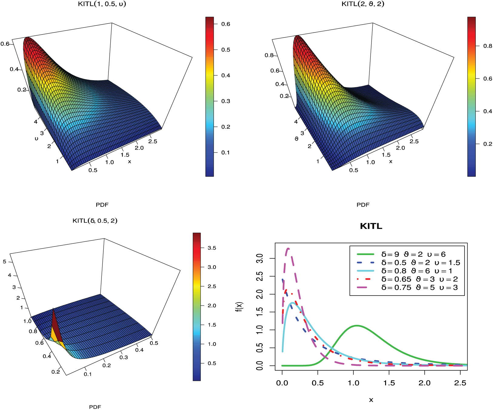
Figure 1: Density function of the KITL distribution

The hazard rate function of KITL distribution is given as follows

h(z;υ)=2δϑυz(1+2z)υ-1(1+z)2υ+1[1-{(1+2z)υ(1+z)2υ}]δ-1(1-[1-{(1+2z)α(1+z)2α}]δ)-1(8)

Plots of the hazard rate function (hrf) of KITL distribution for specific values of parameters are shown in Fig. 2. We conclude that the hrf of KITL distribution has the increasing, decreasing and upside-down shape.

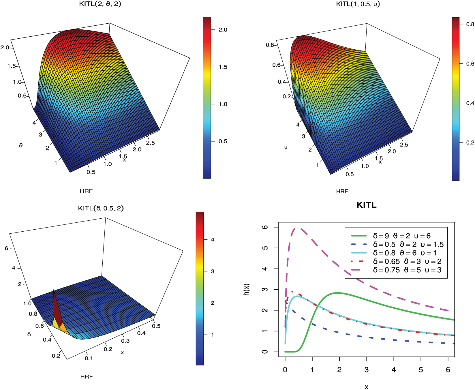
Figure 2: The hrf of the KITL distribution

We are motivated to suggest the KITL model according to: (a) Produce new useful form of ITL with three parameters; (b) discuss several statistical properties (c) introduce more flexible model with decreasing, increasing, and upside-down hazard rate shapes; (d) able to model the COVID-19 data, in Saudi Arabia, Italy, Argentina and Angola, than some other distributions. This article is addressed as follows. Section 2 deals with some important properties. Maximum likelihood (ML) and Bayesian estimators of parameters in presence of Type II censored (T2C) samples are given in Sections 3 and 4 respectively. Monte Carlo simulation is provided in Section 5. Analysis to COVID-19 data sets is carried in Section 6, and conclusions are presented in Section 7.

2  Significant Statistical Measures

Here, some significant properties of KITL distribution, specifically, linear representation of the pdf, quantile function, moments, Rényi and ϖ-entropies, mean residual life, stress-strength reliability are derived.

2.1 Useful Formulae

Here, an important mathematical formula of KITL distribution is provided. Consider the binomial theorem

(1-[1-{(1+2z)υ(1+z)2υ}]δ)ϑ-1=∑s=0∞(-1)s(ϑ-1s)[1-{(1+2z)υ(1+z)2υ}]δs,(9)

in the pdf (7), we obtain

f(z;ς)=∑s=0∞(-1)s(ϑ-1s)2δϑυz(1+2z)υ-1(1+z)2υ+1[1-{(1+2z)υ(1+z)2υ}]δs+δ-1.(10)

Again, employ the binomial expansion in (10), then

f(z;ς)=∑s,k=0∞ψs,k2υ(k+1)z(1+z)-2υ(k+1)-2(1+2z)υ(k+1)-1=∑s,k=0∞ψs,kg(z,υ(k+1)),(11)

where, ψs,k=(-1)s+kδϑ(k+1)(ϑ-1s)(δs+δ-1k), g(z,υ(k+1)) is the density function of ITL distribution with parameter υ(k+1).

2.2 Quantile Function and Median

The KITL distribution is easily simulated by inverting (6) as follows: If U has a uniform distribution on (0, 1), then Z can be obtained from

Q(u)=-2((1-L)1υ-1)+4((1-L)1υ-1)2-4(1-L)1υ((1-L)1υ-1)2(1-L)1υ,(12)

L=(1-(1-u)1ϑ)1δ, and Q(u) is the quantile function of the KITL distribution. Hence, the median zM of the distribution is derived by substituting u = 0.5 in (12).

2.3 Moments Measures

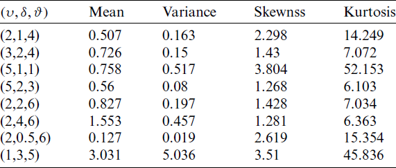
The nth moment for KITL distribution about zero is given by using pdf (11) as follows

E(Zn)=∑s,k=0∞2υ(k+1)ψs,k∫0∞zn+1(1+z)-υ(k+1)-2(1+z1+z)υ(k+1)-1dz,(13)

which gives

E(Zn)=∑s,k,ℓ=0∞Λs,k,ℓB(n+ℓ+2,υ(k+1)-n),(14)

where, Λs,k,ℓ=2υ(k+1)(υ(k+1)-1ℓ)ψs,k and B(⋅,⋅) is the beta function. For, n = 1, 2, 3, 4 we obtain the first four moments around origin. Tab. 1 gives the basic moments measures for particular values of parameters.

Table 1: Some moments values of the KITL distribution

2.4 Incomplete and Conditional Moments

The rth incomplete moment, say Ξr(z) of Z is obtained from (11) as follows

Ξr(Z)=∑s,k=0∞2υ(k+1)ψs,k∫0zzrz(1+z)-υ(k+1)-2(1+z1+z)υ(k+1)-1dz=∑s,k,ℓ=0∞Λs,k,ℓB(r+ℓ+2,υ(k+1)-r,z1+z),(15)

where β(⋅,⋅,x) is the incomplete beta function. Setting r = 1 in (15), we obtain the first incomplete moment as follows

Ξ1(Z)=∑s,k,ℓ=0∞Λs,k,ℓB(ℓ+3,υ(k+1)-1,z1+z)(16)

The Lorenz and Bonferroni curves are useful applications of the first incomplete moment defined by Lo(p)=Ξ1(P)/E(P) and Bo(p)=Lo(p)/F(p) respectively. The mean residual life is another application of Ξ1(t) defined by m1(t)=[1-Ξ1(t)]/S(t)-t.

2.5 Rényi and ϖ-Entropies

Here, we obtain Rényi and ϖ-entropies. The Rényi entropy R(η) of a random variable Z is defined by

R(η)=11-ηLog[∫0∞fη(z)dz],(17)

where, η>0 and η≠1. Substituting (7) in (17), then after some mathematical abbreviations of (f(z;ς))η, we get that:

(f(z;ς))η=∑m,j,ℓ=0∞Am,j,ℓzη+ℓ(1+z)-ηυ-2η-υj-ℓ,(18)

where, Am,j,ℓ=(-1)m+j(η(ϑ-1)m)(η(δ-1)+δmj)(η(υ-1)+υjℓ)(2δϑυ)η.

Substituting (18) in (17), then we obtain the Rényi entropy of KITL distribution as follows:

R(η)=11-ηLog[∑m,j,ℓ=0∞Am,j,ℓ∫0∞zη+ℓ(1+z)-ηυ-2η-υj-ℓdz]=(1-η)-1Log[∑m,j,ℓ=0∞Am,j,ℓB(η+ℓ+1,ηυ+υj+η-1)](19)

The ϖ-entropy, say R(ϖ), is determined by the following relation

R(ϖ)=(ϖ-1)-1Log[1-∫0∞fϖ(z)dz],where ϖ>0 and ϖ≠1.(20)

The ϖ-entropy of the KITL model will be

R(ϖ)=(ϖ-1)-1Log[1-∑m,j,ℓ=0∞Am,j,ℓB(ϖ+ℓ+1,ϖυ+υj+ϖ-1)].(21)

2.6 Stress-Strength Reliability

The stress-strength reliability (SSR) is defined as the probability that the system is strong frequently to beat the stress applied on it. Consider that X1 and X2 are independent stress and strength random variables following the KITL(υ,δ1,ϑ1), and KITL (υ,δ2,ϑ2) distributions, respectively. Then, the SSR of the KITL distribution is defined by

R=P(X2<X1)=∫0∞f1(x;υ,δ1,ϑ1)F2(x;υ,δ2,ϑ2)dx.(22)

Using (6) and (7) in (22), then we get

R=1-∫0∞2δ1ϑ1υx(1+2x)υ-1(1+x)2υ+1[1-{(1+2x)υ(1+x)2υ}]δ1-1(1-[1-{(1+2x)υ(1+x)2υ}]δ1)ϑ1-1×(1-[1-{(1+2x)υ(1+x)2υ}]δ2)ϑ2dx.(23)

Using the binomial expansion in last equation and after simplification we have

R=1-∑m,k,ℓ,j=0∞ϒm,k,ℓ,jB(j+2,υℓ+υ),ϒm,k,ℓ,j=(-1)m+k+ℓ2δ1ϑ1υ(δ1m+δ2k+δ1-1ℓ)(υℓ+υ-1j)(ϑ1-1m)(ϑ2k).(24)

3  Maximum Likelihood Estimation

Here, the ML estimators of the model parameters are determined via T2C scheme. Let z1:n,z2:n,…,zr:n is of T2C sample of size r from a life test of n items whose lifetimes have the KITL distribution with parameters δ, ϑ and υ. Regarding T2C, the test is stopped at specified number of failure r before all n items have failed. Then, the log-likelihood function based on censored observed sample is given by

lnL(z)∝r[ln(δ)+ ln(ϑ)+ ln(υ)]+ϑ(n-r)ln(1-[1-(ℏr:n)υ]δ)+(υ-1)∑j=1r ln(1+2zj:n)-(2υ+1)∑j=1r ln(1+zj:n)+(δ-1)∑j=1r ln[1-(ℏr:n)υ]+(ϑ-1)∑j=1r ln(1-[1-(ℏr:n)υ]δ),(25)

ℏj:n=(1+2zj:n)/(1+zj:n)2. The partial derivatives of lnL(z), denoted by lnℓ, with respect to the model parameters δ, ϑ, and υ are

∂lnℓ∂δ=rδ-ϑ(n-r)ln[1-(ℏr:n)υ][1-(ℏr:n)υ]-δ-1+∑j=1r ln[1-(ℏj:n)υ]-∑j=1r(ϑ-1)ln[1-(ℏj:n)υ][1-(ℏr:n)υ]-δ-1, (26)

∂lnℓ∂ϑ=rϑ+(n-r)ln(1-[1-(ℏr:n)υ]δ)+∑j=1r ln(1-[1-(ℏj:n)υ]δ), (27)

∂lnℓ∂υ=rυ+ϑ(n-r)δ[1-(ℏr:n)υ]δ-1(ℏr:n)υ ln(ℏr:n)1-[1-(ℏr:n)υ]δ-∑j=1r(δ-1)(ℏj:n)υ ln(ℏj:n)1-(ℏj:n)υ-2∑j=1r ln(1+zj:n)+∑j=1r ln(1+2zj:n)+∑j=1r(ϑ-1)δ[1-(ℏj:n)υ]δ-1(ℏj:n)υ ln(ℏj:n)1-[1-(ℏj:n)υ]δ.

The ML estimators of parameters are determined by solving the non-linear Eqs. (26)–(28).

4  Bayesian Estimation

Here, we discuss the Bayesian estimation of the parameters of the KITL distribution. The Bayesian estimator is considered under squared error (SE) loss function which can be defined as;

L(δ̃,δ)=(δ̃-δ)2,L(ϑ̃,ϑ)=(ϑ̃-ϑ)2,L(υ̃,υ)=(υ̃-υ)2,(28)

and linear exponential (LINEX) loss function which can be expressed as

L(δ̃,δ)=eh(δ̃-δ)-h(δ̃-δ)-1,L(ϑ̃,ϑ)=eh(ϑ̃-ϑ)-h(ϑ̃-ϑ)-1,L(υ̃,υ)=eh(υ̃-υ)-h(υ̃-υ)-1;h≠0,δ̃=-1hE(e-hδ),ϑ̃=-1hE(e-hϑ),υ̃=-1hE(e-hυ),(30)

where h reflects the direction and degree of asymmetry.

Assuming that the prior distribution of δ, ϑ, υ denoted by π(δ), π(ϑ), π(υ) have an independent gamma prior distribution. The joint gamma prior density of δ, ϑ, υ can be written as

π(δ,ϑ,υ)∝δa1-1e-b1δϑa2-1e-b2ϑυa3-1e-b3υ;a1,b1,a2,b2,a3,b3>0.(31)

Based on the following likelihood function of the KITL distribution

L(z)∝(1-[1-(ℏr:n)υ]δ)ϑ(n-r)(δϑυ)r∏j=1r〈zj:n(1+2zj:n)υ-1(1+zj:n)2υ+1[1-(ℏj:n)υ]δ-1×(1-[1-(ℏj:n)υ]δ)ϑ-1〉,(32)

and the joint prior density (31), the joint posterior of the KITL distribution with parameters δ, ϑ and υ is

π(δ,ϑ,υ∣z)∝π(δ,ϑ,υ)L(zi∣δ,ϑ,υ).(33)

Then the joint posterior can be written as

π(δ,ϑ,υ∣x)∝δa1-1e-b1δϑa2-1e-b2ϑυa3-1e-b3υ(1-[1-(ℏr:n)υ]δ)ϑ(n-r)(δϑυ)r∏j=1r〈(1+2zj:n)υ-1(1+zj:n)2υ+1[1-(ℏj:n)υ]δ-1(1-[1-(ℏj:n)υ]δ)ϑ-1〉.(34)

To obtain the Bayesian estimators, we can use the Markov Chain Monte Carlo (MCMC) approach. An important sub-class of the MCMC techniques is Gibbs sampling and more general Metropolis within Gibbs samplers. The Metropolis-Hastings (M-H) algorithm together with the Gibbs sampling are the two most popular example of a MCMC method. It’s similar to acceptance rejection sampling, the M-H algorithms consider that, to each iteration of the algorithm, a candidate value can be generated from the KITL distributions. We use the M-H within Gibbs sampling steps to generate random samples from conditional posterior densities of (δ,ϑ,υ) as follows:

π(δ∣z,ϑ,υ)∝δa1-1e-b1δ(1-[1-(ℏr:n)υ]δ)ϑ(n-r)(δ)r∏j=1r〈[1-(ℏj:n)υ]δ-1(1-[1-(ℏj:n)υ]δ)ϑ-1〉, (35)

π(ϑ∣z,δ,υ)∝ϑa2-1e-b2ϑ(1-[1-(ℏr:n)υ]δ)ϑ(n-r)(ϑ)r∏j=1r〈(1-[1-(ℏj:n)υ]δ)ϑ-1〉, (36)

and

π(υ∣z,δ,ϑ)∝υa3+r-1e-b3υ(1-[1-(ℏr:n)υ]δ)ϑ(n-r)×∏j=1r(1+2zj:n)υ-1(1+zj:n)2υ+1[1-(ℏj:n)υ]δ-1(1-[1-(ℏj:n)υ]δ)ϑ-1.(37)

The Bayesian estimates based on SE and LINEX loss functions are obtained in simulation section. For more information, please see as an example [11–13].

5  Simulation Study

A simulation study for KITL model is conducted for samples of sizes n = 20, 50, 100 and the parameters are estimated under complete and T2C samples. The number of failure items; r, is selected for two levels of censoring (LC), as 70% and 90%. 10000 iterations are made to compute the ML estimate (MLE), bias and mean square error (MSE). The observed outcomes are listed in Tabs. 2–4.

Table 2: Bias and MSE of the MLE and Bayesian estimate for KITL model for complete sample

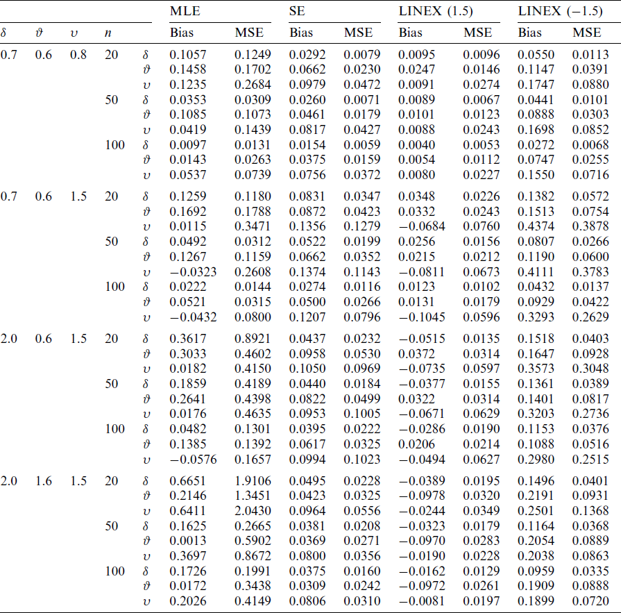
Table 3: Bias and MSE of the MLE and Bayes estimate for KITL model under T2C at LC=70%

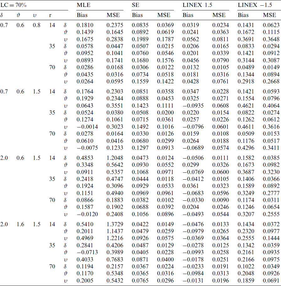
Table 4: Bias and MSE of the MLE and Bayes estimate for KITL model under T2C at LC=90%

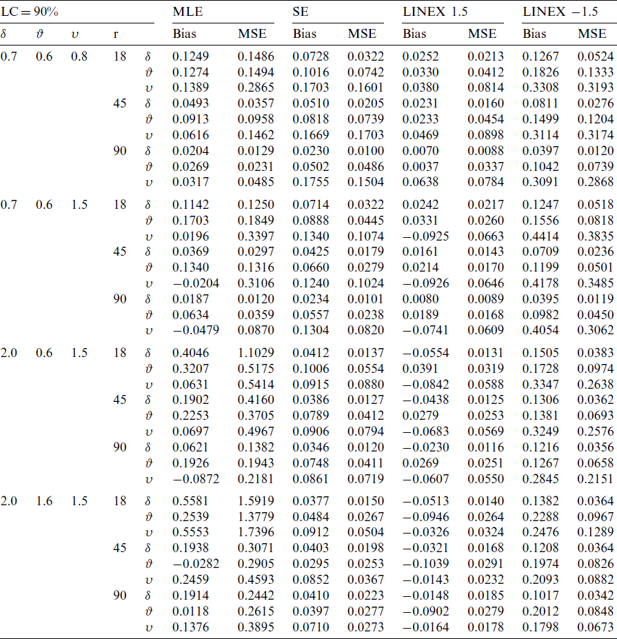
From the above tables, we conclude the following

     i)  As the sample size n increases, the bias decreases.

    ii)  As the sample size n increases, the MSE decreases.

   iii)  As the value of υ increases, the bias and MSE increase.

    iv)  As the value of δ increases, the bias and MSE increase.

     v)  As the value of ϑ increases, the bias and MSE increases.

    vi)  As the level of censoring increases, the bias and MSE decrease.

6  Analysis to COVID-19 Data

In this section, the KITL distribution is fitted to more famous fields of survival times of COVID-19 data with different country including Saudi Arabia, Italy, Argentina, Angola as well as March precipitation data. The data are available at https://covid19.who.int/. Reference [14] used this link to find data of COVID-19 for Egypt. Reference [15] used a deep neural network approach to train networks for estimating the optimal parameters of an SIR model endemicity of COVID-19 in Spain. The KITL model is compared with other some competitive models as, ITL, inverse Weibull (IW), inverse Lomax (IL), inverse Kumaraswamy (IK) and Topp Leone inverted Kumaraswamy (TLIK) distributions (see [16]).

Tabs. 5–9 provide values of Cramér–von Mises (W*), Anderson–Darling (A*) and Kolmogorov–Smirnov (KS) statistics for all models fitted based on five real data sets. In addition, these tables contain the MLEs and standard errors (SEs) (appear in parentheses) of the parameters for the considered models. We compare the fits of the KITL model with the ITL, IW, IL, IK and TLIK models (see Tabs. 5–9). The fitted KITL, pdf and cdf of the five data sets are displayed in Figs. 3–7, respectively. These figures indicate that the KITL distribution gets the lowest values of W*, A*, KS among all fitted models.

Table 5: MLE and statistical measures for COVID-19 data in Argentina

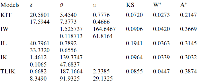
Table 6: MLE and statistical measures for COVID-19 data in Saudi Arabia country

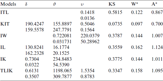
Table 7: MLE and statistical measures for COVID-19 data in Italy country

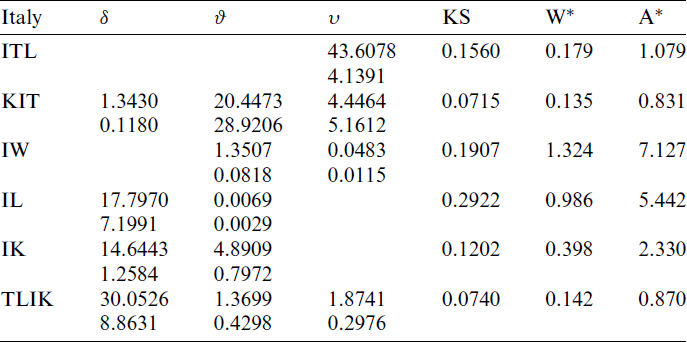
Table 8: MLE and statistical measures for COVID-19 data in Angola

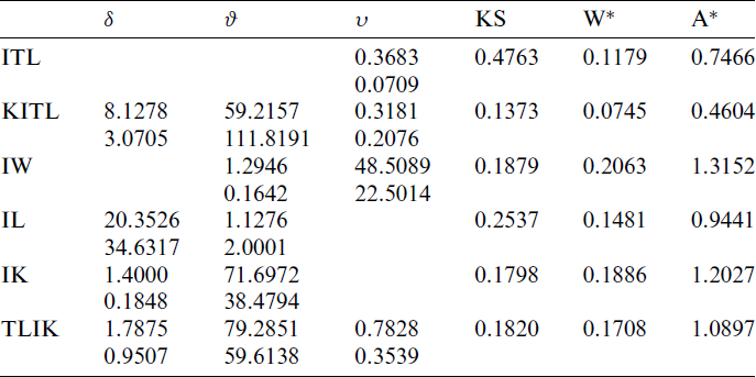
Table 9: MLE and statistical measures for March precipitation data

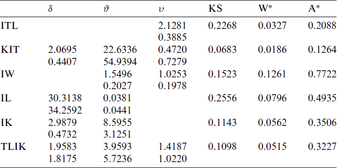
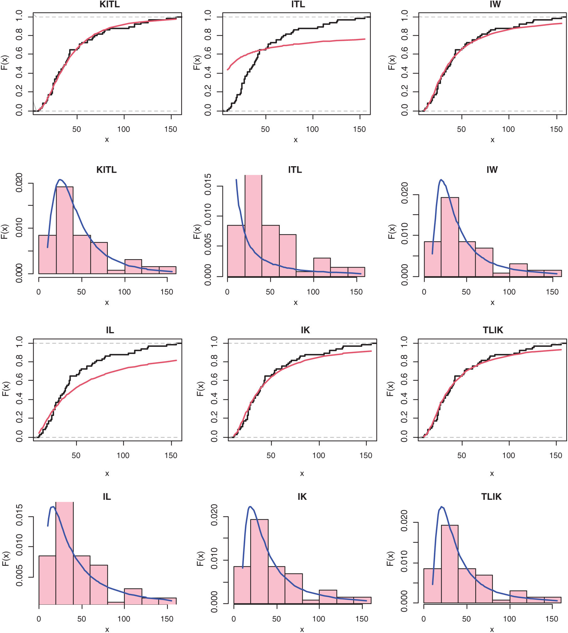
Figure 3: The histogram and estimated cdf for all models of COVID-19 in Argentina country

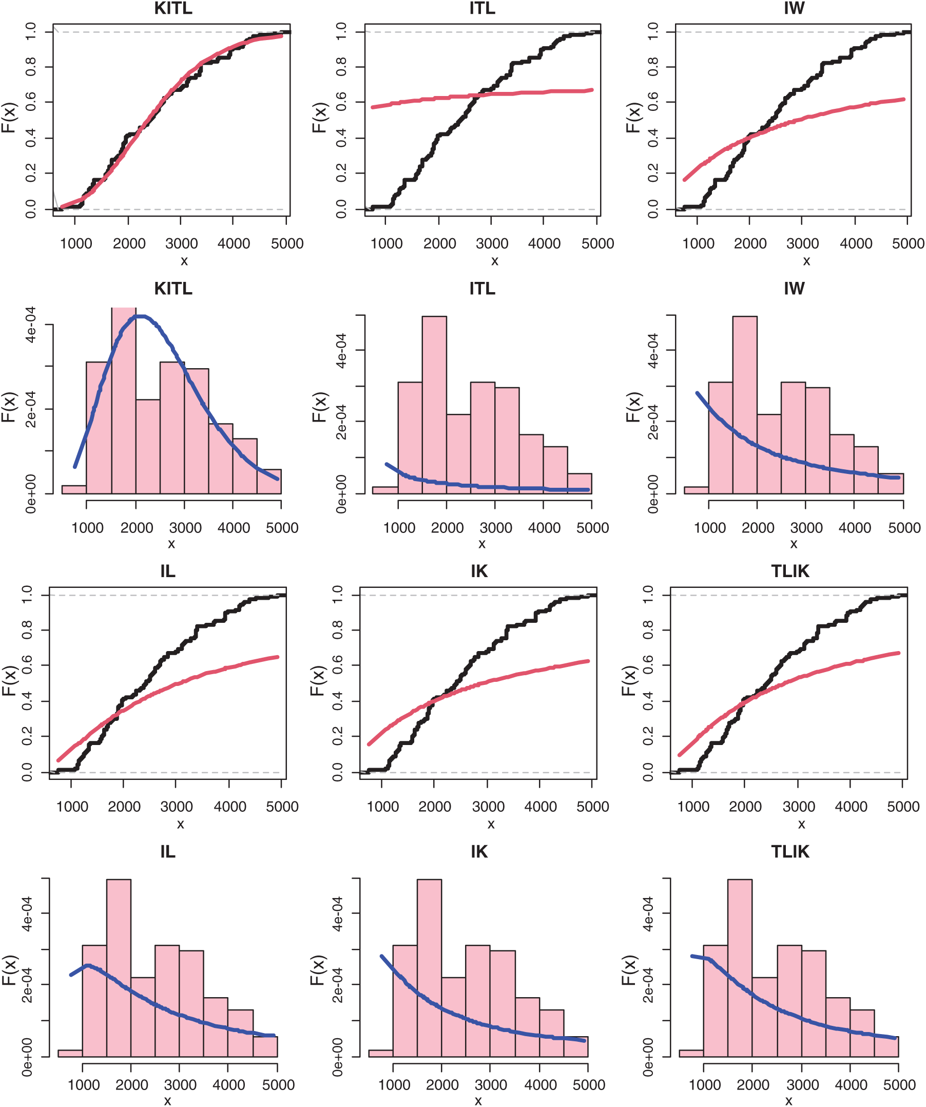
Figure 4: The histogram and estimated cdf for all models of COVID-19 in Saudi Arabia country

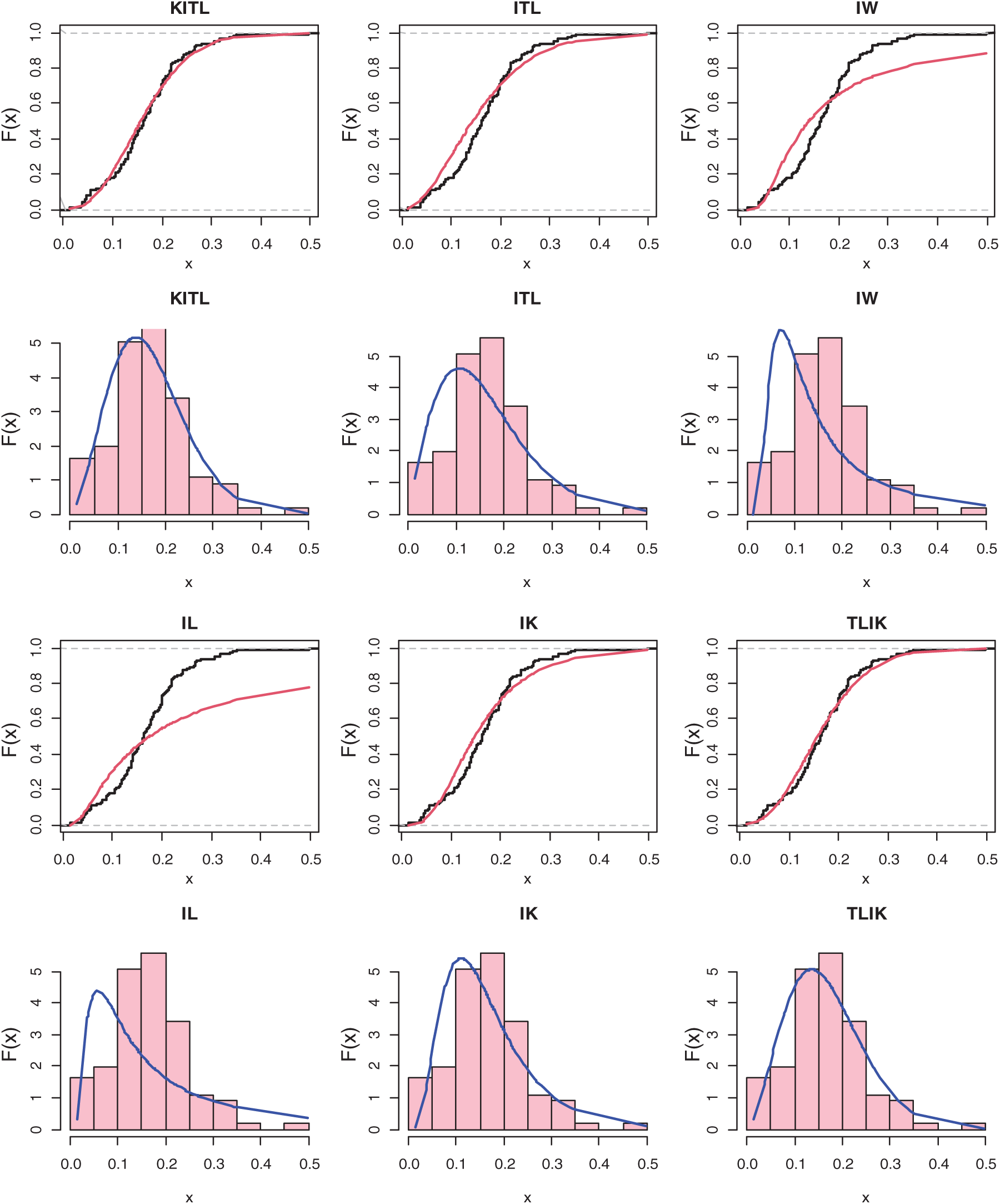
Figure 5: The histogram and estimated cdf for all models of COVID-19 in Italy

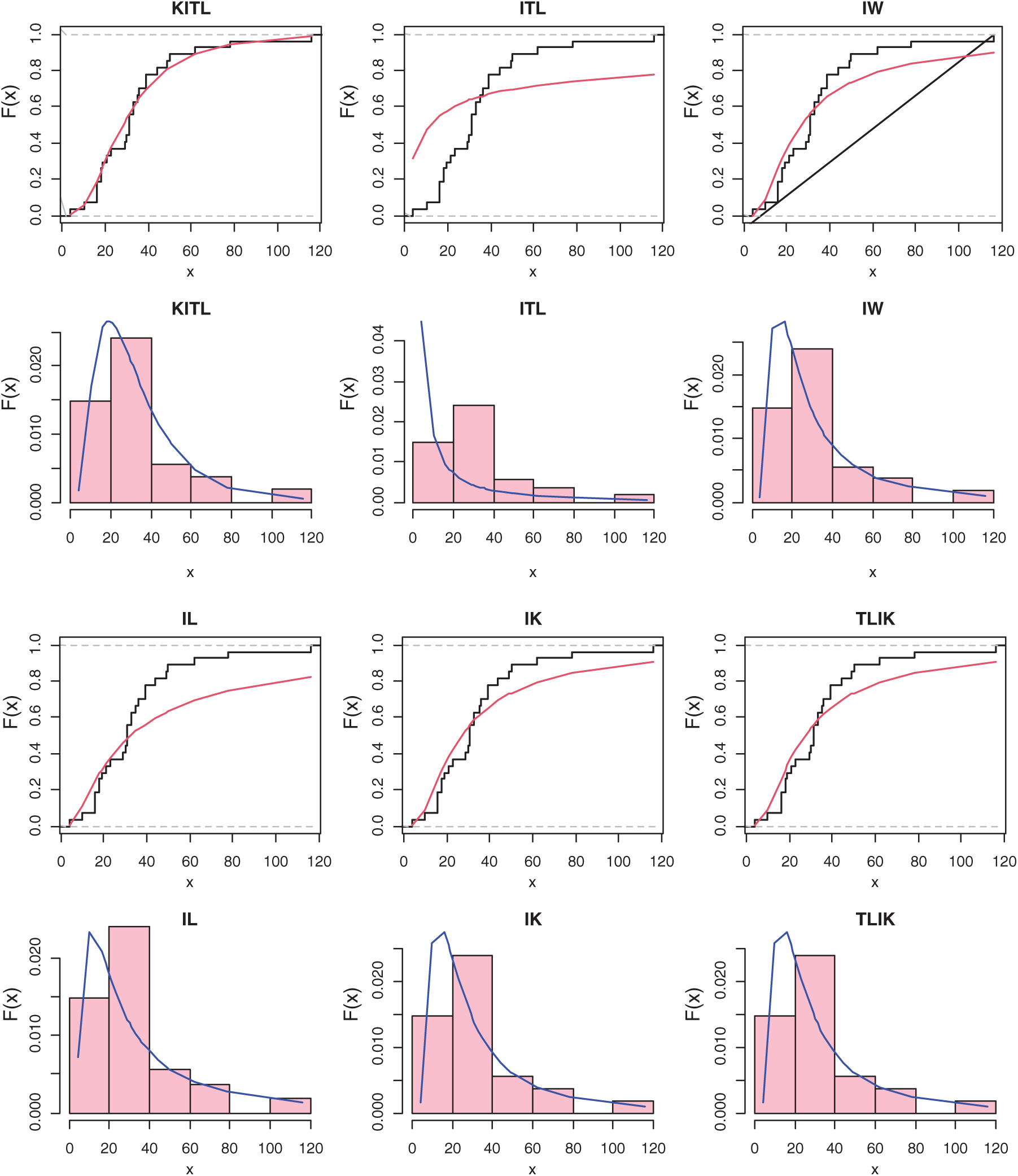
Figure 6: The histogram and estimated cdf for all models of COVID-19 in Angola

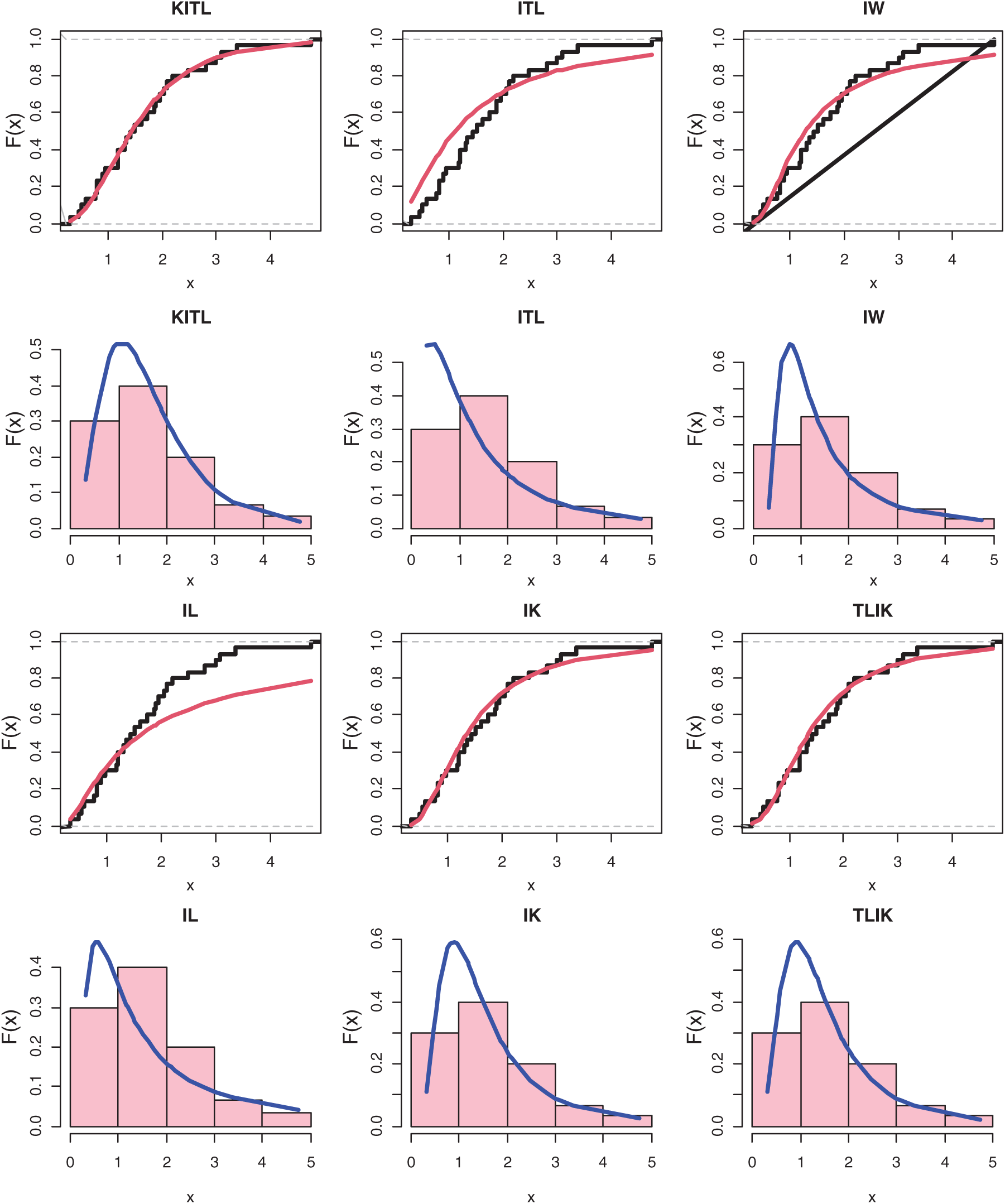
Figure 7: CDF and PDF for different distribution for March precipitation data

6.1 Argentina Data

The following COVID-19 data represent the daily new deaths which belong to Argentina in 65 days recorded from 1 June to 4 August 2020: 20, 11, 19, 10, 18, 27, 27, 14, 14, 28, 19, 24, 31, 30, 17, 23, 20, 24, 43, 25, 25, 13, 24, 33, 36, 39, 43, 25, 25, 28, 38, 27, 53, 40, 50, 37, 33, 79, 52, 53, 42, 38, 31, 41, 67, 61, 85, 61,71, 42, 35, 145, 80, 111, 105, 125, 66, 43, 126, 118, 111, 155, 77, 69, and 55.

Tab. 5 gives the MLEs, SEs and the statistics measures for all models. Tab. 5 shows that the KITL model gives the smallest values for the K-S, W* and A* statistics among all fitted models.

Furthermore, we plot the histogram, estimated pdf plots for all models for data of Argentina in Fig. 3.

6.2 Saudi Arabia Data

The following COVID-19 data belong to Saudi Arabia in 109 days recorded from 17 April to 4 August 2020 (data of daily new cases): 762, 1088, 1122, 1132, 1141, 1147, 1158, 1172, 1197, 1223, 1258, 1266, 1289, 1325, 1344, 1351, 1357, 1362, 1552, 1573, 1581, 1595, 1618, 1629, 1644, 1645, 1686, 1687, 1701, 1704, 1759, 1793, 1815, 1869, 1877, 1881, 1897, 1905, 1911, 1912, 1931, 1966, 1968, 1975, 1993, 2039, 2171, 2201, 2235, 2238, 2307, 2331, 2378, 2399, 2429, 2442, 2476, 2504, 2509, 2532, 2565, 2591, 2593, 2613, 2642, 2671, 2691, 2692, 2736, 2764, 2779, 2840 2852, 2994, 3036, 3045, 3121, 3123, 3139, 3159, 3183, 3288, 3366, 3369, 3372, 3379, 3383, 3392, 3393, 3402, 3580, 3717, 3733, 3921, 3927, 3938, 3941, 3943, 3989, 4128, 4193, 4207, 4233, 4267, 4301, 4387, 4507, 4757, 4919.

Tab. 6 gives the MLEs, SEs and the statistics measures for all models for Saudi Arabia data. We conclude that the KITL is an adequate model for these data compared to other models.

Furthermore, the histogram and estimated cdf plots for all models for data of Saudi Arabia are plotted in Fig. 4.

6.3 Italy Data

The considered COVID-19 data belong to Italy of 111 days that are recorded from 1 April to 20 July 2020. This data formed of daily new deaths divided by daily new cases. The data are as follows: 0.2070, 0.1520, 0.1628, 0.1666, 0.1417, 0.1221, 0.1767, 0.1987, 0.1408, 0.1456, 0.1443, 0.1319, 0.1053, 0.1789, 0.2032, 0.2167, 0.1387, 0.1646, 0.1375, 0.1421, 0.2012, 0.1957, 0.1297, 0.1754, 0.1390, 0.1761, 0.1119, 0.1915, 0.1827, 0.1548, 0.1522, 0.1369, 0.2495, 0.1253, 0.1597, 0.2195, 0.2555, 0.1956, 0.1831, 0.1791, 0.2057, 0.2406, 0.1227, 0.2196, 0.2641, 0.3067, 0.1749, 0.2148, 0.2195, 0.1993, 0.2421, 0.2430, 0.1994, 0.1779, 0.0942, 0.3067, 0.1965, 0.2003, 0.1180, 0.1686, 0.2668, 0.2113, 0.3371, 0.1730, 0.2212, 0.4972, 0.1641, 0.2667, 0.2690, 0.2321, 0.2792, 0.3515, 0.1398, 0.3436, 0.2254, 0.1302, 0.0864, 0.1619, 0.1311, 0.1994, 0.3176, 0.1856, 0.1071, 0.1041, 0.1593, 0.0537, 0.1149, 0.1176, 0.0457, 0.1264, 0.0476, 0.1620, 0.1154, 0.1493, 0.0673, 0.0894, 0.0365, 0.0385, 0.2190, 0.0777, 0.0561, 0.0435, 0.0372, 0.0385, 0.0769, 0.1491, 0.0802, 0.0870, 0.0476, 0.0562, 0.0138.

Tab. 7 provides the MLEs, SEs and the statistics measures for all models for Italy data. We conclude that the KITL is an adequate model for these data compared to other models.

Also, the histogram and estimated cdf plots for all models for data of Italy country are plotted in Fig. 5.

6.4 Angola Data

The considered COVID19 data represent the daily new cases which are belonging to Angola of 27 days recorded from 8 July to 3 August 2020. The data are as follows: 33, 10, 62, 4, 21, 23, 19, 16, 35, 31, 31, 49, 18, 44, 30, 33, 39, 29, 36, 16, 18, 50, 78, 31, 39, 16, 116.

Tab. 8 presents the MLEs, SEs and the statistics measures for all models for Angola data. We conclude that the KITL is an adequate model for these data compared to other models.

Fig. 6 gives the histogram and estimated cdf plots for all models for data of Angola country.

6.5 March Precipitation Data in Minneapolis/St Paul

Reference [17] reported data that contain 30 observations of the March precipitation (in inches) in Minneapolis/St Paul. The observed values are: 0.77, 1.74, 0.81, 1.20, 1.95, 1.20, 0.47, 1.43, 3.37, 2.20, 3.00, 3.09, 1.51, 2.10, 0.52, 1.62, 1.31, 0.32, 0.59, 0.81, 2.81, 1.87, 1.18, 1.35, 4.75, 2.48, 0.96, 1.89, 0.90, 2.05.

Tab. 9 presents the MLEs, SEs and the statistics measures for all models for March precipitation data. We conclude that the KITL is an adequate model for these data compared to other models. Fig. 7 gives the histogram and estimated cdf plots for all models for data of March precipitation.

7  Conclusions

This article formulates a generalization of inverted Topp–Leone distribution, named as Kumaraswamy inverted Topp–Leone distribution. Some statistical properties of the KITL distribution are provided. Bayesian and ML methods of estimation are considered. The Bayesian estimator is deduced under LINEX and SE loss functions. Monte Carlo simulation study is designed to assess the performance of estimates. Generally, we conclude that the Bayesian estimates are preferable than the corresponding other estimates in approximately most of the situations. Five real data of COVID-19 obtained from Saudi Arabia, Italy, Argentina, and Angola as well as March precipitation data are considered and they showed that KITL distribution is an adequate model for these data compared with other competitive distributions.

Funding Statement: The authors received no specific funding for this study.

Conflicts of Interest: The authors declare that they have no conflicts of interest to report regarding the present study.

References

 1.  A. M. Abd AL-Fattah, A. A. El-Helbawy and G. R. Al-Dayian. (2017). “Inverted Kumaraswamy distribution: Properties and estimation,” Pakistan Journal of Statistics, vol. 33, no. 1, pp. 37–61. [Google Scholar]

 2.  K. V. P. Barco, J. Mazucheli and V. Janeiro. (2017). “The inverse power Lindley distribution,” Communications in Statistics-Simulation and Computation, vol. 46, no. 8, pp. 6308–6323. [Google Scholar]

 3.  R. Calabria and G. Pulcini. (1990). “On the maximum likelihood and least-squares estimation in the inverse Weibull distribution,” Statistica Applicata, vol. 2, no. 1, pp. 53–66. [Google Scholar]

 4.  A. S. Hassan and M. Abd-Allah. (2019). “On the inverse power Lomax distribution,” Annals of Data Science, vol. 6, no. 2, pp. 259–278. [Google Scholar]

 5.  A. S. Hassan and R. Mohamed. (2019). “Parameter estimation for inverted exponentiated Lomax distribution with right censored data,” Gazi University Journal of Science, vol. 32, no. 4, pp. 1370–1386. [Google Scholar]

 6.  V. K. Sharma, S. K. Singh, U. Singh and V. Agiwal. (2015). “The inverse Lindley distribution: A stress-strength reliability model with application to head and neck cancer data,” Journal of Industrial and Production Engineering, vol. 32, no. 3, pp. 162–173. [Google Scholar]

 7.  M. H. Tahir, G. M. Cordeiro, S. Ali, S. Dey and A. Manzoor. (2018). “The inverted Nadarajah–Haghighi distribution: Estimation methods and applications,” Journal of Statistical Computation and Simulation, vol. 88, no. 14, pp. 2775–2798. [Google Scholar]

 8.  A. S. Hassan and S. G. Nassr. (2018). “The inverse Weibull generator of distributions: Properties and applications,” Journal of Data Sciences, vol. 16, no. 4, pp. 732–742. [Google Scholar]

 9.  A. S. Hassan, M. Elgarhy and R. Ragab. (2020). “Statistical properties and estimation of inverted Topp–Leone distribution,” Journal of Statistics Applications & Probability, vol. 9, no. 2, pp. 319–331. [Google Scholar]

10. G. M. Cordeiro and M. de Castro. (2011). “A new family of generalized distributions,” Journal of Statistical Computation and Simulation, vol. 81, no. 7, pp. 883–893. [Google Scholar]

11. M. Nassar, O. Abo-Kasem, C. Zhang and S. Dey. (2018). “Analysis of Weibull distribution under adaptive type-II progressive hybrid censoring scheme,” Journal of the Indian Society for Probability and Statistics, vol. 19, no. 1, pp. 25–65. [Google Scholar]

12. H. H. Ahmad and E. Almetwally. (2020). “Marshall-Olkin generalized Pareto distribution: Bayesian and non Bayesian estimation,” Pakistan Journal of Statistics and Operation Research, vol. 16, no. 1, pp. 21–33. [Google Scholar]

13. E. M. Almetwally, H. M. Almongy and A. El sayed Mubarak. (2018). “Bayesian and maximum likelihood estimation for the Weibull generalized exponential distribution parameters using progressive censoring schemes,” Pakistan Journal of Statistics and Operation Research, vol. 15, no. 4, pp. 853–868. [Google Scholar]

14. E. M. Almetwally, H. M. Almongy and A. H. Saleh. (2020). “Managing risk of spreading “COVID-19” in Egypt: Modelling using a discrete Marshall–Olkin generalized exponential distribution,” International Journal of Probability and Statistics, vol. 9, no. 2, pp. 33–41. [Google Scholar]

15. G. N. Baltas, F. A. Prieto, M. Frantzi, C. R. Garcia-Alonso and P. Rodriguez. (2020). “Data driven modelling of coronavirus spread in Spain,” Computers Materials & Continua, vol. 64, no. 3, pp. 1343–1357. [Google Scholar]

16. H. Reyad, F. Jamal, S. Othman and N. Yahia. (2019). “The Topp Leone generalized inverted Kumaraswamy distribution: Properties and applications,” Asian Research Journal of Mathematics, vol. 13, no. 1, pp. 1–15. [Google Scholar]

17. D. Hinkley. (1977). “On quick choice of power transformation,” Journal of the Royal Statistical Society: Series C (Applied Statistics), vol. 26, no. 1, pp. 67–69. [Google Scholar]

This work is licensed under a Creative Commons Attribution 4.0 International License, which permits unrestricted use, distribution, and reproduction in any medium, provided the original work is properly cited.